• Aucun résultat trouvé

The iterative reweighted Mixed-Norm Estimate for spatio-temporal MEG/EEG source reconstruction

N/A
N/A
Protected

Academic year: 2021

Partager "The iterative reweighted Mixed-Norm Estimate for spatio-temporal MEG/EEG source reconstruction"

Copied!
12
0
0

Texte intégral

(1)

HAL Id: hal-01079530

https://hal.archives-ouvertes.fr/hal-01079530v2

Submitted on 27 Jul 2016

HAL is a multi-disciplinary open access

archive for the deposit and dissemination of

sci-entific research documents, whether they are

pub-lished or not. The documents may come from

teaching and research institutions in France or

abroad, or from public or private research centers.

L’archive ouverte pluridisciplinaire HAL, est

destinée au dépôt et à la diffusion de documents

scientifiques de niveau recherche, publiés ou non,

émanant des établissements d’enseignement et de

recherche français ou étrangers, des laboratoires

publics ou privés.

Distributed under a Creative Commons Attribution - NonCommercial - NoDerivatives| 4.0

International License

spatio-temporal MEG/EEG source reconstruction

Daniel Strohmeier, Yousra Bekhti, Jens Haueisen, Alexandre Gramfort

To cite this version:

Daniel Strohmeier, Yousra Bekhti, Jens Haueisen, Alexandre Gramfort. The iterative reweighted

Mixed-Norm Estimate for spatio-temporal MEG/EEG source reconstruction. IEEE Transactions on

Medical Imaging, Institute of Electrical and Electronics Engineers, 2016, �10.1109/TMI.2016.2553445�.

�hal-01079530v2�

(2)

The iterative reweighted Mixed-Norm Estimate

for spatio-temporal MEG/EEG source reconstruction

Daniel Strohmeier, Yousra Bekhti, Jens Haueisen, and Alexandre Gramfort

Abstract—Source imaging based on magnetoencephalography (MEG) and electroencephalography (EEG) allows for the non-invasive analysis of brain activity with high temporal and good spatial resolution. As the bioelectromagnetic inverse problem is ill-posed, constraints are required. For the analysis of evoked brain activity, spatial sparsity of the neuronal activation is a common assumption. It is often taken into account using convex constraints based on the l1-norm. The resulting source estimates

are however biased in amplitude and often suboptimal in terms of source selection due to high correlations in the forward model. In this work, we demonstrate that an inverse solver based on a block-separable penalty with a Frobenius norm per block and a l0.5-quasinorm over blocks addresses both of

these issues. For solving the resulting non-convex optimization problem, we propose the iterative reweighted Mixed Norm Estimate (irMxNE), an optimization scheme based on iterative reweighted convex surrogate optimization problems, which are solved efficiently using a block coordinate descent scheme and an active set strategy. We compare the proposed sparse imaging method to the dSPM and the RAP-MUSIC approach based on two MEG data sets. We provide empirical evidence based on simulations and analysis of MEG data that the proposed method improves on the standard Mixed Norm Estimate (MxNE) in terms of amplitude bias, support recovery, and stability.

Index Terms—Electrophysical imaging, brain, inverse meth-ods, magnetoencephalography, electroencephalography, struc-tured sparsity.

I. INTRODUCTION

Source imaging with magnetoencephalography (MEG) and electroencephalography (EEG) delivers insights into the active brain with high temporal and good spatial resolution in a non-invasive way [1]. It is based on solving the bioelectromagnetic inverse problem, which is a high dimensional ill-posed regression problem. In order to render Copyright (c) 2016 IEEE. Personal use of this material is permitted. However, permission to use this material for any other purposes must be obtained from the IEEE by sending a request to pubs-permissions@ieee.org. This work was supported by the German Research Foundation (Ha 2899/21-1), the European Union (FP7-PEOPLE-2013-IAPP 610950), the EDF and Jacques Hadamard Mathematical Foundation (Gaspard Monge Program for Optimization and operations research), the French National Research Agency (ANR-14-NEUC-0002-01), and the National Institutes of Health (R01 MH106174).

D. Strohmeier is with the Institute of Biomedical Engineering and Informatics, Technische Universi¨at Ilmenau, Ilmenau, Germany; e-mail: daniel.strohmeier@tu-ilmenau.de

Y. Bekhti is with the LTCI, CNRS, T´el´ecom ParisTech, Universit´e Paris-Saclay, Paris, France; e-mail: yousra.bekhti@telecom-paristech.fr

J. Haueisen is with the Institute of Biomedical Engineering and Informatics, Technische Universi¨at Ilmenau, Ilmenau, Germany and the Biomagnetic Center, Department of Neurology, Jena University Hospital, Jena, Germany; e-mail: jens.haueisen@tu-ilmenau.de

A. Gramfort is with the LTCI, CNRS, T´el´ecom ParisTech, Universit´e Paris-Saclay, Paris, France and the NeuroSpin, CEA Paris-Saclay, Bat. 145, Gif-sur-Yvette Cedex, France; e-mail: alexandre.gramfort@telecom-paristech.fr

its solution unique, constraints have to be imposed reflecting a priori assumptions on the neuronal sources. In the past, several source reconstruction techniques have been proposed, which are based on the assumption that only a few focal brain regions are involved in a specific cognitive task. Inverse methods favoring sparse focal source configurations to explain the MEG/EEG signals include parametric [2], scanning [3]–[6], and imaging approaches [7]–[12]. These techniques, which are partly used in clinical routine, are suitable e.g. for analyzing evoked responses or epileptic spike activity. Classic MEG/EEG source imaging technique using sparsity-inducing penalties are the Selective Minimum Norm Method [7] or Minimum Current Estimate (MCE) [13]. Both approaches are based on the Lasso [14], i.e., regularized regression with an l1-norm penalty, which is

a convex surrogate for the optimal, but NP hard l0-norm

regularized regression problem. To reduce the sensitivity to noise and avoid discontinuous, scattered source activations [8], mixed norms such as the l2,1-mixed-norm used in Group

Lasso [15] or Group Basis Pursuit [16] can be applied. The idea is to take the spatio-temporal characteristics of neuronal activity into account by imposing structured sparsity in space or time [8], [9], [17], [18]. We refer to [19] for a general review on group selection in high-dimensional models. A prominent example is the Mixed-Norm Estimate (MxNE) proposed in [9], which extends the MCE to multiple measurement vector problems by applying a block-separable convex penalty. Each block represents the source activation over time of a dipole with free orientation at a specific source location. Spatial sparsity is promoted by an l1-norm

penalty over blocks, whereas a Frobenius norm per block promotes stationary source estimates, i.e., a source with a non-zero amplitude at one time instant has a non-zero amplitude during the full time window of interest [9], [20]. The Frobenius norm also prevents the orientations of the free orientation dipoles from being biased towards the coordinate axes [21]. These convex approaches allow for fast algorithms with guaranteed global convergence. However, the resulting source estimates are biased in amplitude and often suboptimal in terms of support recovery [22], which is impaired by the high spatial correlation of the MEG/EEG forward model. As shown e.g. in the field of compressed sensing, promoting sparsity by applying non-convex penalties, such as logarithmic or lp-quasinorm penalties with 0 < p < 1,

improves support reconstruction in terms of feature selection, amplitude bias, and stability [22]–[24]. Several approaches for solving the resulting non-convex optimization problem have been proposed including generalized shrinkage [25], iterative reweighted l1 [22], [26]–[28], or iterative reweighted

(3)

l2 optimization [29]–[33]. See [27], [34] for a review of

these approaches for single and multiple measurement vector problems. Several MEG/EEG sparse source imaging techniques based on iterative reweighted l2 optimization

have been proposed [29], [35]–[38]. An iterative reweighted l1 optimization technique for EEG source imaging was

proposed in [39], which however does not impose structured sparsity and applies a fixed orientation constraint [40]. In this paper, we propose the iterative reweighted Mixed-Norm Estimate (irMxNE), a novel MEG/EEG sparse source imaging approach based on the framework of iterative reweighted l1,

which promotes structured sparsity to improve MEG/EEG source reconstruction. A preliminary version of this method was presented in [41]. Similar approaches have recently been proposed in other fields of research [34], [42]. The irMxNE is based on a non-convex block-separable penalty, which combines a Frobenius norm per block and an l0.5-quasinorm

over blocks. The non-convex objective function is minimized iteratively by computing a sequence of weighted MxNE problems. For solving the convex surrogate problems, we propose a new computationally efficient strategy, which combines block coordinate descent [27], [43], [44] and a forward active set strategy with convergence controlled by means of the duality gap, which converges significantly faster than the original MxNE algorithm proposed in [9]. We provide information on the integration of different source orientation constraints [40] and discuss specific problems of MEG/EEG source imaging such as depth bias compensation and amplitude bias correction. We present empirical evidence using simulations and analysis of two experimental MEG data sets that the proposed method outperforms MCE and MxNE in terms of amplitude bias, active source identification, and stability. Finally, we compare the proposed approach with the dSPM [45] and RAP-MUSIC method [5] based on two MEG data sets.

Notation: We mark vectors with bold letters, a ∈ RN, and

matrices with capital bold letters, A ∈ RN ×M. The transpose

of a vector or matrix is denoted by aT and AT. The scalar a[i]

is the ith element of a. A[i, :] corresponds to the ith row and

A[:, j] to the jth column of A. kAk

Froindicates the Frobenius

norm, and kAk the spectral norm of a matrix.

II. MATERIALS ANDMETHODS A. The inverse problem

The MEG/EEG forward problem describes the linear rela-tionship between the MEG/EEG measurements M ∈ RN ×T (N number of sensors, T number of time instants) and the source activation X ∈ R(SO)×T (S number of source loca-tions, O number of orthogonal dipoles per source location with O = 1 if source orientation is postulated, e.g. using the cortical constraint [46], and typically O = 3 otherwise). The model then reads:

M = GX + E , (1) where G ∈ RN ×(SO)is the gain or leadfield matrix, a known instantaneous mixing matrix, which links source and sensor

signals. E is the measurement noise, which is assumed to be additive, white, and Gaussian, E[:, j] ∼ N (0, I) for all j. This assumption is acceptable on the basis of a proper spatial whitening of the data using an estimate of the noise covariance [47]. As SO  N , the MEG/EEG inverse problem is ill-posed and constraints have to be imposed on the source activation matrix X to render the solution unique. By partition-ing X into S blocks Xs∈ RO×T, where each Xs represents

the source activation at a specific source location s over time and across O orthogonal current dipoles, we can apply a penalty term P(X) promoting block sparsity by combining a Frobenius norm per block and a l0.5-quasinorm penalty over

blocks. The optimization problem reads:

b X = arg min X∈RSO×T 1 2kM − GXk 2 Fro+ P(X) b X = arg min X∈RSO×T 1 2kM − GXk 2 Fro+ λ S X s=1 Ps(Xs) b X = arg min X∈RSO×T 1 2kM − GXk 2 Fro+ λ S X s=1 pkXskFro , (2)

where λ > 0 is the regularization parameter balancing the data fit and penalty term. Similar to the constraint applied in MxNE [9], P(X) promotes source estimates with only a few focal sources that have non-zero activations during the entire time interval of interest. The Frobenius norm per block Xs, which combines l2-norm penalties over time and

orientation as proposed in [8], [13], [20], imposes stationarity of the source estimate and prevents the source orientations from being biased towards the coordinate axes [21]. The l0.5-quasinorm penalty promotes spatial sparsity.

B. Iterative reweighted Mixed Norm Estimate

The proposed block-separable regularization functional is an extension of the l2,p-quasinorm penalty with 0 < p < 1 used

in [22], [26], [27], [32]. These works showed, based on the framework of Difference of Convex functions programming or Majorization-Minimization algorithms, that the resulting non-convex optimization problem can be solved by iteratively solving a sequence of weighted convex surrogate optimization problems with weights being defined based on the previous es-timate. The convex surrogate problem is obtained by replacing the non-decreasing concave function Ps(Xs) with a convex

upper bound using a local linear approximation at the current estimate. By solving this sequence of surrogate problems, the value of the non-convex objective function decreases, but without guarantee for convergence to a global minimum. The cost function in Eq. (2) can thus be minimized by computing the sequence of convex problems given in Eq. (3). The weights for the kth iteration are obtained from the previous source estimate bX(k−1). Intuitively, sources with high amplitudes in the (k-1)th iteration will be less penalized in the kth iteration

(4)

and therefore further promoted. b X(k)= arg min X∈RSO×T 1 2kM − GXk 2 Fro+ λ X s kXskFro 2 r Xb (k−1) s Fro = arg min X∈RSO×T 1 2kM − GXk 2 Fro+ λ X s 1 w(k)[s]kXskFro (3) As each iteration is equivalent to solving a weighted MxNE problem, we call this optimization scheme the iterative reweighted MxNE (irMxNE). Due to the non-convexity of the optimization problem in Eq. (2), the procedure is sensitive to the initialization of w(k)[s]. In this paper, we use w(1)[s] = 1

for all s as proposed in [26]. Consequently, the first iteration of irMxNE is equivalent to solving a standard MxNE problem. As each iteration of the iterative scheme in Eq. (3) solves a convex problem with guaranteed global convergence, the initialization of X has no influence on the final solution. X can thus be chosen arbitrarily and we use warm starts for improving the computation time. For sources with k bX(k)s kFro = 0, Eq. (3)

has an infinite regularization term. Typically, a smoothing pa-rameter  is added to avoid weights to become zero [22], [26], [31]. Here, we reformulate the weighted MxNE subproblem and apply the weights without epsilon smoothing by scaling the gain matrix with a weighting matrix W(k) as given in

Eq. (4). After convergence, we reapply the scaling to eX(k)to

obtain the final estimate bX(k).

e X(k)= arg min X∈RSO×T 1 2kM − GW (k)Xk2 Fro+ λ X s kXskFro = arg min X∈RSO×T 1 2kM − G (k)Xk2 Fro+ λ X s kXskFro b X(k)= W(k)Xe(k) (4) with W(k) ∈ RSO×SO being a diagonal matrix, which is

computed according to Eq. (5):

W(k)= diag(w(k)⊗ 1(O)) with w(k)[s] = 2 r Xb (k−1) s Fro, (5)

where 1(O)∈ RO is a vector of ones and ⊗ is the Kronecker

product. In each MxNE iteration, we restrict the source space to source locations with w(k)[s] > 0 to reduce the

computation time.

We control the global convergence of each weighted MxNE subproblems in Eq. (4) by monitoring the duality gap. For details on convex duality in the context of optimization with sparsity-inducing penalties, we refer to [48]. In the following, we summarize the rationale for this stopping criterion. For a general minimization problem, the minimum of the primal objective function Fp(X) is bounded below

by the maximum of the associated dual objective function Fd(Y), i.e., Fp(X∗) ≥ Fd(Y∗), where X∗ and Y∗ are

the optimal solutions of the primal and dual problem. The duality gap η = Fp(X) − Fd(Y) ≥ 0, where X and Y are

the current values of the primal and dual variable, is thus non-negative and provides an upper bound on the difference between Fp(X) and Fp(X∗). If strong duality holds, the

duality gap at the optimum is zero. To use this stopping criterion in practice, we need to derive the dual problem and choose a good feasible dual variable Y given a value of X, which allows for η = 0 at the optimum.

Due to Slater’s conditions [49], strong duality holds for the MxNE subproblem and we can check convergence of an iterative optimization scheme solving Eq. (4) by computing the current duality gap η(i) = Fp(X(i)) − Fd(Y(i)) ≥ 0. Based

on the Fenchel-Rockafellar duality theorem [50], the dual objective function associated to the primal objective function

Fp(X) = 1 2kM − GXk 2 Fro+ λΩ(X) = 1 2kM − GXk 2 Fro+ λ X s kXskFro

is given in Eq. (6). For a detailed derivation, we refer to [9]. Fd(Y) = − 1 2kYk 2 Fro+ Tr Y TM − λΩGTY/λ (6) where Tr indicates the trace of a square matrix, and Ω∗ the Fenchel conjugate of Ω, which is the indicator function of the associated dual norm. As shown in [9], a natural mapping from the primal to the dual space is given by a scaling of the residual

e

Y = M − GX. This is motivated by the fact that the solution of the dual problem at the optimum is proportional to the residual, which follows from the associated KKT conditions [9]. The scaling is done according to Eq. (7) such that the dual variable Y satisfies the constraint of Ω∗.

Y = eY.maxmax s G T sYe Fro . λ, 1 (7) In practice, we terminate the iterative optimization scheme for solving MxNE, when the estimate at the ithinner iteration X(i)is -optimal with  = 10−6, i.e., η(i)< 10−6. According

to [9], this is a conservative choice provided that the data is scaled by spatial pre-whitening.

For solving the weighted MxNE subproblems, we propose a block coordinate descent (BCD) scheme [43], which, for the problem at hand, converges faster than the Fast Iterative Shrinkage-Thresholding algorithm (FISTA) proposed earlier in [9] (cf. section III-B). A BCD scheme for solving the Group LASSO was proposed in [27], [44]. The subproblem per block has a closed form solution, which involves applying the group soft-thresholding operator, the proximity operator associated to the l2,1-mixed-norm [9]. Accordingly, the closed form solution

for the BCD subproblems solving the MxNE problem can be derived, which is given in Eq. (8).

X(k)s = X(k−1)s + µ[s]GTs M − GX(k−1) e X(k)s = eX(k)s max   1 − µ[s]λ max X (k) s Fro, µ[s]λ  , 0    (8)

(5)

The step length µ[s] for each BCD subproblem is deter-mined by µ[s] = L−1s with Ls= kGTsGsk being the Lipschitz

constant of the data-fit restricted to the sthsource location. This

step length is typically larger than the step length applicable in iterative proximal gradient methods, which is upper-bounded by the inverse of L = kGTGk. Pseudo code for the BCD

scheme is shown in Algorithm 1. Algorithm 1 MxNE with BCD

Require: M, G, X, µ, λ > 0,  > 0, and S. 1: Initialization: η = Fp(X) − Fd(Y)

2: while η ≥  do 3: for s = 1 to S do

4: Xs←− Solve Eq. (8) with X, µ, and M

5: end for

6: η = Fp(X) − Fd(Y)

7: end while

The BCD scheme is typically applied using a cyclic sweep pattern, i.e., all blocks are updated in a cyclic order in each iteration. However, as the penalty term in Eq. (2) promotes spatial sparsity, most of the blocks of bX are zero. We can thus reduce the computation time by primarily updating blocks, that are likely to be non-zero, while keeping the remaining blocks at zero. For this purpose, data-dependent sweep patterns (such as greedy approaches based on steepest descent [51], [52]) or active set strategies [53], [54] can be applied. In this paper, we combine BCD with a forward active set strategy proposed in [9], [54]. Pseudo code for the proposed MxNE solver is provided in Algorithm 2.

Algorithm 2 MxNE with BCD and active set strategy Require: M, G, λ > 0,  > 0, and S. 1: Initialization: X = 0, A = {}, η = Fp(X) − Fd(Y) 2: for s = 1 to S do 3: µ[s] = kGTsGsk−1 4: end for 5: while η ≥  do 6: A∗⊆ {s | kGTs(M − GX)kFro> λ} 7: A = A ∪ A∗

8: Define GA and XAby restricting G and X to A 9: XbA←− Solve Algorithm 1 with µ, GAand X0= XA

10: X = bXAfor s ∈ A, else 0 11: η = Fp(X) − Fd(Y)

12: end while

We start by estimating an initial active set of sources A by evaluating the Karush-Kuhn-Tucker (KKT) optimality conditions, which state that Xbs= 0 if

kGT

s(M − GX)kFro≤ λ [9]. We select the N sources

as the initial active set, which violate this condition the most (we use N = 10 in practice). Subsequently, we restrict the source space to the sources in A and estimate bXAby solving Eq. (4) with convergence controlled by the duality gap. After convergence of this restricted optimization problem, we check whether bXA is also an -optimal solution for the original optimization problem (without restricting the source space to A) by computing the corresponding duality gap η assuming

that all sources, which are not part of the active set, have zero activation. If bXA is not an -optimal solution indicated by η ≥ , we re-evaluate the KKT optimality conditions and update the active set A by adding the N sources with the highest score. We then repeat the procedure with warm start.

We terminate irMxNE when k bX(k) − bX(k−1)k

∞ < τ

with a user specified threshold τ , which we set to 10−6 in practice. The proposed optimization algorithm for irMxNE is fast enough to allow its usage in practical MEG/EEG applications. Full pseudo code for irMxNE is provided in Algorithm 3.

Algorithm 3 Iterative reweighted MxNE Require: M, G, λ > 0,  > 0, τ > 0, and K.

1: Initialization: W(1)= I, bX(1)

2: for k = 1 to K do 3: G(k)= GW(k)

4: Xe(k) ←− Solve Algorithm 2 with G(k) and X(k) 5: Xb(k)= W(k)Xe(k)

6: if k bX(k)− bX(k−1)k

∞< τ then

7: break 8: end if

9: W(k+1) ←− Solve Eq. 5 with bX(k)

10: end for

C. Source constraints and bias

1) Source orientation: The proposed BCD scheme is ap-plicable for MEG/EEG inverse problems without and with orientation constraint. For imposing a loose orientation con-straint [40], we apply a weighting matrix K = diag([1, ρ, ρ]) to each block of the gain matrix Gs ∈ RN ×3 with Gs[:, 1]

corresponding to the dipole orientated normally to the cortical surface, and Gs[:, 2] and Gs[:, 3] to the two tangential dipoles.

The weighting parameter 0 < ρ ≤ 1 controls up to which angle the rotating dipole may deviate from the normal direction [20], [40]. The orientation-weighted gain matrix eG is hence defined as eG = G I(S)⊗ K, where I(S) ∈ RS×S is the identity

matrix. Since the penalty in Eq. (8) does not promote sparsity along orientations, the irMxNE result is not biased towards the coordinate axes [21]. When the source orientation is postulated a priori (e.g. normal to the cortical surface), each block Xs

corresponds to the activation of a fixed dipole. Consequently, the Frobenius norm per block can be replaced by the l2-norm

of the source activation of the corresponding fixed dipole. 2) Depth bias compensation: Due to the attenuation of the bioelectromagnetic field with increasing distance between source and sensor, deep sources require higher source ampli-tudes to generate sensor signals of equal strength compared to superficial sources. Consequently, inverse methods, which are based on constraints penalizing the source amplitudes, have a bias towards superficial sources. In order to compensate this bias, each block of the gain matrix is weighted a priori. Here, we apply the depth bias compensation proposed in [55], which computes the weights used for depth bias compensation based on the SVD of the gain matrix.

(6)

3) Amplitude bias compensation: Source activation es-timated with source reconstruction approaches based on lp-quasinorms with 0 < p ≤ 1, such as MxNE and

ir-MxNE, show a varying degree of amplitude bias due to the inherent shrinkage. The standard practice for compensating the amplitude bias consists in computing the least squares fit after restricting the source space to the support of bX, which is typically an over-determined optimization problem. In contrast, we apply the debiasing approach proposed in [20], which preserves the source characteristics and orientations estimated with irMxNE by estimating a scaling factor for each source, which is constrained to be above 1 and constant over orientation and time. The bias corrected source estimate eX is computed using D as eX = D bX, where the diagonal scaling matrix D is estimated based on the convex problem:

b

D = arg min

D

kM−G(D⊗I(O)) bXk2Fro s.t.

(

Dij≥ 1, i = j

Dij= 0, i 6= j

D. Simulation setup

We compare MCE, MxNE and irMxNE in terms of ampli-tude bias, support recovery, and stability using simulated au-ditory evoked fields. The simulation, which was repeated 100 times, is based on a real gain matrix computed with a three-shell boundary element model using 4699 cortical sources with fixed orientation (normal to the cortical surface), and a 306-channels Elekta Neuromag Vectorview system (Elekta Neuromag Oy, Helsinki, Finland) with 102 magnetometers and 204 gradiometers. The sampling rate was set to 1 kHz and we restricted the analysis to the time window from 60 ms to 150 ms. We generated single trials by activating two dipolar sources, one in each transverse temporal gyrus, with Gaussian functions peaking at 100 ms and 110 ms with a peak amplitude of 55 nAm and 45 nAm, Xsim. Background activity

was generated by ten dipolar sources placed randomly on the cortical surface. Each dipole was activated with filtered white noise with a peak amplitude of 100 nAm. The filter coefficients were determined by fitting an auto-regressive process of order 5 to real baseline MEG data [20]. By averaging 100 single tri-als, the SNR of the evoked response, which we compute using spatial whitened data as SNR = kMsignalk2Fro/kMnoisek2Fro, was

set to SNR = 2.63 ± 0.46. Source reconstruction was com-puted without orientation constraint, where none of the dipoles used to generate the gain matrix was oriented perpendicularly to the cortical surface. All methods were applied with different regularization parameters λ given as a percentage of the respective λmax, which is the smallest regularization parameter

leading to an empty active set [9]. We evaluate the source reconstruction performance by means of the true and false positives counts. We consider a source to be a true positive, if its geodesic distance along the cortical surface from the true source location is less than 1 cm. A value of 1 cm is what would be considered an acceptable localization error for most neuroscience applications. Moreover, we present the active set size and the root mean square error in the sensor space, RMSE = kGXsim− G bXkFro. To evaluate the stability of the

reconstructed support, we compute Krippendorff’s alpha [56].

E. Experimental MEG data

We evaluate the performance of MxNE and irMxNE using data from the MIND multi-site MEG study [57]–[59]. We use two different data sets from one exemplary subject, auditory evoked fields (AEF) and somatosensory evoked fields (SEF), recorded using the 306-channels Elekta Neuromag Vectorview system. A detailed description of the data and paradigms can be found in [57]–[59]. For the AEF data set, we report results for AEFs evoked by left auditory stimulation with pure tones of 500 Hz. The analysis window for source estimation was chosen from 50 ms to 200 ms based on visual inspection of the evoked data to capture the dominant N100m component. For the SEF data set, we analyzed SEFs evoked by bipolar electri-cal stimulation (0.2 ms in duration) of the left median nerve. To capture the main peaks of the evoked response and to exclude the strong stimulus artifact, the analysis window was chosen from 18 ms to 200 ms based on visual inspection. Following the standard pipeline from the MNE software [60], signal preprocessing for both data sets consisted of signal-space projection for suppressing environmental noise, and baseline correction using pre-stimulus data (from -200 ms to -20 ms). Epochs with peak-to-peak amplitudes exceeding predefined rejection parameters (3 pT for magnetometers, 400 pT/m for gradiometers, and 150 V for EOG) were assumed to be af-fected by artifacts and discarded. This resulted in 96 (AEF) and 294 (SEF) artifact-free epochs, which were resampled to 500 Hz. The gain matrix was computed using a set of 7498 cortical locations, and a three-layer boundary element model. The stability of the source reconstruction was tested using a resampling technique. For each data set, we generated 100 random sets of epochs by randomly selecting 80% of all avail-able epochs without replacement. The noise covariance matrix for spatial whitening was estimated for each subsample using pre-stimulus data (from -200 ms to -20 ms). We applied both MxNE and irMxNE on the average of each random set without orientation constraint. Due to the lack of a ground truth, the source reconstruction performance is evaluated by means of the Goodness of Fit (GOF) and the active set size. To compare results with well established source reconstruction techniques, we compute the dSPM solution [45] without orientation con-straint and the RAP-MUSIC estimate [5] for both data sets using the MNE-Python software [61]. For RAP-MUSIC, we use single-dipole and two-dipole independent topographies to address the problem of correlated sources [4]. A similar idea is pursued e.g. by dual core beamformers [62]. The correlation threshold was set to 0.95 as proposed by Mosher et al. [4]. The rank of the signal subspace was determined by thresholding the eigenvalues of the data covariance based on an estimate of the noise variance. As we apply a spatial whitening, the threshold was set to 1.

III. RESULTS A. Simulation study

The results of the simulation study (100 repetitions) for different regularization parameters (from 5 to 100 % of λmax)

are presented in Fig. 1. The source space contained 4699 sources and one source per hemisphere was active indicated

(7)

0

1

2

3

4

5

6

7

True positives

(left A1)

(a)

10

10

-2 -1

10

0

10

1

10

2

10

3

Active set size

(d)

0

1

2

3

4

5

6

True positives (right A1)

(b)

4

2

6

8

10

12

14

16

18

RMSE

(e)

0

20

40

60

80

100

/

max

(%)

10

-2

10

10

-1 0

10

1

10

2

10

3

False positives

(c) MCE MxNE irMxNE

0

20

40

60

80

100

/

max

(%)

0.0

0.1

0.2

0.3

0.4

0.5

0.6

0.7

0.8

0.9

Kr

ipp

en

do

rff

s

α

(f) MCE MxNE irMxNE

Fig. 1: Results of the simulation study based on simulated AEFs for MCE, MxNE and irMxNE. The source space contained a total of 4699 sources and the simulation was repeated 100 times: (a) mean true positive count (left A1), (b) mean true positive count (right A1), (c) mean false positive count, (d) mean active set size, (e) mean RMSE without (solid) and with (dashed) debiasing, and (f) Krippendorff’s α.

by the horizontal dashed lines in Fig. 1a and b. True posi-tive counts above this threshold indicate suboptimally sparse source estimates, whereas counts close to zero indicate false negatives. We can see that the irMxNE approach provides the best support recovery. It allows to reconstructs single dipoles in both regions of interest, whereas MCE and MxNE find multiple correlated sources. Particularly for low values of λ, MCE and MxNE overestimate the size of the active set leading to a large number of false positives, whereas irMxNE generates significantly less false positives. The mean active set size confirms that irMxNE provides the sparsest result of all three methods. The mean RMSE is shown in Fig. 1e. While all methods profit from the debiasing procedure, the effect on irMxNE is less pronounced compared to the other methods indicating a reduced amplitude bias. The best result is obtained with irMxNE. Krippendorff’s α indicates that the support reconstructed with irMxNE is more stable compared to MCE or MxNE. The source estimate is thus less dependent on the epochs used for generating the evoked response. B. Experimental MEG data

1) Auditory evoked fields: We first compare the perfor-mance of the proposed BCD scheme for solving the weighted MxNE with the Fast Iterative Shrinkage Thresholding Al-gorithm (FISTA) [63], a proximal gradient method used in [9]. Both methods were applied with and without active set strategy. All computations were performed on a computer with a 2.4 GHz Intel Core 2 Duo processor and 8 GB RAM. The computation times as a function of λ are presented in Fig. 2. The BCD scheme outperforms FISTA both with and without active set strategy. Combining the BCD scheme and

the active set strategy reduces the computation time by a factor of 100 and allows to compute the MxNE on real MEG/EEG data in a few seconds. Since subsequent MxNE iterations are significantly faster due to the restriction of the source space, irMxNE also runs in a few seconds on real MEG/EEG source localization problems. 10 20 30 40 50 60 70 80 90 100 / max(%) 100 101 102 103 104 105 Time (s) FISTA FISTA-AS BCD BCD-AS

Fig. 2: Computation time as a function of λ for MxNE on real MEG data (free orientation) using BCD and FISTA with (solid) and without (dashed) active set strategy.

We applied MxNE and irMxNE (with and without debiasing) with different regularization parameters λ to 100 AEF data sets generated by averaging randomly selected subsets of epochs. The mean GOF around the N100m component (from 90 ms to 150 ms) and the mean active set size are presented in Fig. 3 as a function of λ. We can see that the debiasing procedure has a strong effect on MxNE, whereas the GOF of the irMxNE result is only slightly improved indicating less amplitude bias. Debiased MxNE and irMxNE yield similar GOFs with similar plateaus, but irMxNE provides a sparser, i.e., simpler model.

(8)

10

20

30

40

50

60

70

80

90

100

Mean GOF

(a)

10 20 30 40 50 60 70 80 90 100

/

max

(%)

0

5

10

15

20

25

Active set size

(b)

MxNE irMxNE

Fig. 3: Mean GOF, and active set size for MxNE and irMxNE without (solid) and with (dashed) debiasing for the AEF data.

The selection probability for all sources being, at least once, part of the active set obtained with MxNE or irMxNE is shown in Fig. 4. MxNE selects multiple sources with high probability within each region of interest, which is a consequence of the correlated design. The irMxNE approach is more selective and provides sparser source estimates. Moreover, the number of false positives, i.e., sources outside of the regions of interest, is lower for irMxNE, particularly for low values of λ.

Fig. 4: Source selection probability for the AEF data set using MxNE (left) and irMxNE (right). The plot is restricted to sources that are active in at least one random subsample. The colored patches on the inflated brain indicate regions of interest based on anatomical labels (green, yellow, red). Source indices, which are in the regions of interest, are highlighted by corresponding color marks. The transversal temporal gyrus is indicated in green.

Exemplary source reconstructions for debiased MxNE and

irMxNE are illustrated in Fig. 5. For comparison, we present a RAP-MUSIC estimate based on single- and two-dipole independent topographies [4], [5]. The maximum dSPM score [45] per source is shown as an overlay on each cortical surface. MxNE with λ/λmax= 60% shows activation in both

primary auditory cortices with main peaks around 110 ms corresponding to the N100m component. The activation on the right hemisphere is however split into two highly correlated dipoles, which are partly located on the wrong side of the Sylvian fissure. Increasing λ does not fix the latter issue, since dipoles in the left primary auditory cortex are eliminated before actually erasing spurious activity on the right hemisphere. The loss of the active source in the left auditory cortex is also indicated by the drop of the GOF in Fig. 3. The size of the signal subspace for RAP-MUSIC was estimated to be 50 by the thresholding procedure. Being based on an empirical estimate of the data covariance, this procedure tends to overselect the rank of the signal subspace [5] and the RAP-MUSIC estimate depends on the correlation threshold. With the setting proposed in [4], only two independent topographies, a single- and a two-dipole topography, yield sufficient subspace correlations. The dipoles are reconstructed close to the primary auditory cortex on both hemispheres. The GOF of the three-dipole model is 86.7%. Using single- and two-dipole topographies provides better RAP-MUSIC estimates than using only single-dipole topographies. The irMxNE with λ/λmax = 60%, which

converged after 10 iterations, reconstructs single dipoles in both primary auditory cortices. Intuitively, the green and blue sources, which are the strongest sources according to MxNE with λ/λmax = 60%, are favored at the next iteration of

the reweighted scheme pruning out the source on the wrong side of the Sylvian fissure present in the MxNE result. The estimated source locations roughly match the peaks of the dSPM estimate. The source estimate obtained with dSPM or similar linear inverse methods (sLORETA, MNE, etc.) is however spatially smeared. To reduce the smearing of the dSPM estimate, one could increase the threshold, yet it would make it time dependent and certainly too high to see weaker sources. Alternatively, post-processing is generally required, e.g. by defining regions of interest, to improve interpretability. Note also that, in contrast to dSPM, source amplitudes obtained with irMxNE are moments of electrical dipoles expressed in nAm, which is similar to dipole fitting procedures [2]. The GOF of the two-dipole model obtained with irMxNE is 81.9% and thus only slightly lower than the three-dipole model obtained with RAP-MUSIC. 2) Somatosensory evoked fields: We applied MxNE and irMxNE (with and without debiasing) with different regularization parameters to 100 averaged random subsets of epochs of the SEF data set. The mean GOF and the corresponding active set size for MxNE and irMxNE (with and without debiasing) as a function of the regularization parameter λ are shown in Fig. 6. We can see again that irMxNE yields significantly sparser source estimates, which however allow for a better GOF compared to MxNE. The GOFs of the MxNE and irMxNE results with and without

(9)

(a) MxNE with λ/λmax= 60% (b) MxNE with λ/λmax= 70%

(c) RAP-MUSIC (2 independent topographies) (d) irMxNE with λ/λmax= 60%

Fig. 5: Source reconstruction results using AEFs evoked by left auditory stimulation. The estimated source locations for MxNE (a, b), RAP-MUSIC (c) and irMxNE (d), indicated by colored spheres, and the cor-responding time courses are color-coded. The maximum of the dSPM estimate per source, which is thresholded for visual-ization purposes, is shown as an overlay on each cortical surface.

debiasing illustrate also that the irMxNE source estimates are less biased in amplitude.

0

10

20

30

40

50

60

70

80

90

Mean GOF

(a)

10 20 30 40 50 60 70 80 90 100

/

max

(%)

0

5

10

15

20

25

30

35

40

Active set size

(b)

MxNE irMxNE

Fig. 6: Mean GOF, and active set size for MxNE and irMxNE without (solid) and with (dashed) debiasing for the SEF data.

Fig. 7 presents the selection probability for all sources, which are non-zero in at least one MxNE or irMxNE estimate. The irMxNE typically selects only one source per region of interest for different values of λ. The number of false positives is also significantly lower. These results confirm the findings obtained from the AEF data set in section III-B1. The stability analysis reveals also that the source in the ipsilateral secondary somatosensory cortex (iS2) is less stable compared to the

contralateral sources, which might be caused by its relatively weak field pattern [12].

Fig. 7: Selection probability for sources obtained with MxNE (left) and irMxNE (right) for the SEF data. The plot is restricted to sources that are active in at least one random subsample. The colored patches on the inflated brain indicate regions of interest based on anatomical labels (green, yellow, red). Source indices, which are in the regions of interest, are highlighted by corresponding color marks.

(10)

MxNE and irMxNE for selected regularization parameters. As in section III-B1, we show a RAP-MUSIC estimate and added the maximum dSPM score per source as an overlay to all subfigures. MxNE with λ/λmax= 40% reconstructs dipoles

in the contralateral primary somatosensory cortex (cS1), the contralateral and ipsilateral secondary somatosensory cortices (cS2 and iS2), and the posterial parietal cortex (cPPC). The source locations roughly coincide with the main peaks of the dSPM estimate. As for the AEF data set, the source activation per region is split into several correlated dipoles. An increase of the regularization parameter results in a loss of physiologically meaningful source activity such as activation in iS2, which is visible in the dSPM estimate. The relevance of this activation is also indicated by the drop of the GOF in Fig. 6. The signal subspace estimation for RAP-MUSIC yields a signal subspace size of 43. Hence, the RAP-MUSIC estimate depends on the choice of the correlation threshold. For our settings, four independent topographies, two single- and two two-dipole topographies, are above the subspace correlation threshold. Dipoles are reconstructed in all relevant areas. The activation in cS1 is split into several dipoles, probably due to the fixed orientation source model applied in RAP-MUSIC. The GOF of this six-dipole model is 82,6%. The RAP-MUSIC estimate benefits from using single and two-dipole topographies. The irMxNE approach with λ/λmax= 40%

converged after 14 reweightings. The resulting source estimate contains four single dipoles representing activation in each of the four regions. The GOF of the four-dipole model obtained with irMxNE is 81.4% and thus higher than the GOF of the corresponding MxNE estimate and only slightly lower than the GOF of the six-dipole model obtained with RAP-MUSIC.

IV. DISCUSSION ANDCONCLUSION

In this work, we presented irMxNE, an MEG/EEG in-verse solver based on regularized regression with a non-convex block-separable penalty. The non-non-convex optimiza-tion problem is solved by iteratively solving a sequence of weighted MxNE problems, which allows for fast algorithms and global convergence control at each iteration. We proposed a new algorithm for solving the MxNE surrogate problems combining BCD and a forward active set strategy, which significantly decreases the computation time compared to the original MxNE algorithm [9]. This new algorithm makes the proposed iterative reweighted optimization scheme applicable for practical MEG/EEG applications. The approach is also applicable to other block-separable non-convex penalties such as the logarithmic penalty proposed in [22] by adapting the definition of the weights in Eq. (5). The irMxNE method is designed for offline source reconstruction, which is still the main application of MEG/EEG source imaging in research and clinical routine. However, we are aware of a growing interest in real-time brain monitoring [64]. New techniques such as parallel BCD schemes [51], clustering approaches [65], and safe rules [66] can help to further reduce the computation time. As proposed in [22], [26], the first iteration of irMxNE is equivalent to computing the standard MxNE. Consequently, the irMxNE result is at least as sparse as the MxNE estimate.

The iterative reweighting procedure can thus be considered as a post-processing for MxNE improving source recovery, stability, and amplitude bias. This was confirmed by empirical results based on simulations and two MEG data sets. We attribute this to the spatial correlation and the poor condi-tioning of the forward operator in MEG/EEG source analysis. An alternative approach to improve the conditioning of the inverse problem based on clustering the columns of the gain matrix is presented in [65], which however affects the spatial resolution. The source locations reconstructed by irMxNE roughly coincided with the main peaks of the dSPM estimate, which demonstrate that the proposed inverse solver can present a simple and easy-to-interpret spatio-temporal picture of the active sources. The models reconstructed with RAP-MUSIC provided a slightly higher goodness of fit, but contained more active sources. We found that RAP-MUSIC benefits from using single-dipole and two-dipole independent topographies. The use of higher-order source models, which are limited to a small number of correlated sources, however signifi-cantly increases the computational complexity, particularly for source spaces with high resolution. Approaches improving the computation time of RAP-MUSIC are presented in [64]. In contrast, irMxNE makes no assumption on the number of correlated sources. Its computation time is not dramatically affected by the resolution of the source space. Model selection for sparse source imaging approaches, which amounts here to choosing the regularization parameter, is a critical aspect. Automatic approaches based on minimizing the prediction error such as cross-validation tend to overestimate the number of active sources and increase the false positive rate. Here, we selected the regularization parameter based on the GOF and the size of the active set. A similar procedure is used e.g. in sequential dipole fitting. The development of an automatic model selection procedure for the proposed inverse solver is future work. In particular, approaches maximizing model sta-bility are an interesting alternative [67], [68]. Model selection is however a general issue in MEG/EEG source reconstruction. In our comparison with RAP-MUSIC, we found e.g. that the size of the signal subspace and the correlation threshold have a strong influence on the final source estimate. Due to the limited number of samples, we can only obtain an empirical estimate of the data covariance, which involves the risk of overestimating the size of the signal subspace using the thresholding procedure. The correlation threshold is used to switch to higher order source models and to account for noise components in the signal subspace. Similar to MxNE, irMxNE assumes that the locations of active sources is constant over time. Hence, it should be applied to data, for which this model assumption is approximately true, e.g., by selecting intervals of interest or applying a moving window approach. To go beyond stationary sources, the reconstruction of non-stationary focal source activation can be improved by applying sparsity constraints in the time-frequency domain such as in the TF-MxNE [20]. Preliminary results on the application of non-convex regularization for such models based on iterative reweighting procedures were presented in [69]. The irMxNE solver is available in the MNE-Python package [61].

(11)

(a) MxNE with λ/λmax= 40% (b) MxNE with λ/λmax= 55%

(c) RAP-MUSIC (4 independent topographies) (d) irMxNE with λ/λmax= 40%

Fig. 8: Source reconstruction results using SEFs evoked by electrical stimulation of the left median nerve. The es-timated source locations for MxNE (a, b), RAP-MUSIC (c) and irMxNE (d), indicated by colored spheres, and the cor-responding time courses are color-coded. The maximum of the dSPM estimate per source, which is thresholded for visual-ization purposes, is shown as an overlay on each cortical surface.

ACKNOWLEDGMENT

The authors would like to thank M. S. H¨am¨al¨ainen for providing the experimental MEG data sets.

REFERENCES

[1] S. Baillet, J. C. Mosher, and R. M. Leahy, “Electromagnetic brain mapping,” IEEE Signal Proc. Mag., vol. 18, no. 6, pp. 14–30, Nov. 2001.

[2] M. Scherg and D. Von Cramon, “Two bilateral sources of the late AEP as identified by a spatio-temporal dipole model,” Electroencephalogr. Clin. Neurophysiol., vol. 62, no. 1, pp. 32–44, Jan. 1985.

[3] J. C. Mosher, P. S. Lewis, and R. M. Leahy, “Multiple dipole modeling and localization from spatio-temporal MEG data,” IEEE Trans. Biomed. Eng., vol. 39, no. 6, pp. 541–557, June 1992.

[4] J. C. Mosher and R. M. Leahy, “Recursive MUSIC: a framework for EEG and MEG source localization,” IEEE Trans. Biomed. Eng., vol. 45, no. 11, pp. 1342–1354, Jan. 1998.

[5] ——, “Source localization using recursively applied and projected (RAP) MUSIC,” IEEE Trans. Signal Process., vol. 47, no. 2, pp. 332– 340, Feb. 1999.

[6] X.-L. Xu, B. Xu, and B. He, “An alternative subspace approach to EEG dipole source localization,” Phys. Med. Biol., vol. 49, no. 2, p. 327, Jan. 2004.

[7] K. Matsuura and Y. Okabe, “Selective minimum-norm solution of the biomagnetic inverse problem,” IEEE Trans. Biomed. Eng., vol. 42, no. 6, pp. 608–615, June 1995.

[8] W. Ou, M. S. H¨amal¨ainen, and P. Golland, “A distributed spatio-temporal EEG/MEG inverse solver,” NeuroImage, vol. 44, no. 3, pp. 932–946, Feb. 2009.

[9] A. Gramfort, M. Kowalski, and M. S. H¨am¨al¨ainen, “Mixed-norm estimates for the M/EEG inverse problem using accelerated gradient methods.” Phys. Med. Biol., vol. 57, no. 7, pp. 1937–1961, Apr. 2012. [10] F. Lucka, S. Pursiainen, M. Burger, and C. Wolters, “Hierarchical bayesian inference for the EEG inverse problem using realistic FE head models: Depth localization and source separation for focal primary currents,” NeuroImage, vol. 61, no. 4, pp. 1364–1382, Apr. 2012.

[11] D. Wipf and S. Nagarajan, “A unified bayesian framework for MEG/EEG source imaging,” NeuroImage, vol. 44, no. 3, pp. 947–966, Feb. 2009.

[12] A. Sorrentino, L. Parkkonen, A. Pascarella, C. Campi, and M. Piana, “Dynamical MEG source modeling with multi-target bayesian filtering,” Hum. Brain Mapp., vol. 30, no. 6, pp. 1911–1921, June 2009. [13] K. Uutela, M. S. H¨am¨al¨ainen, and E. Somersalo, “Visualization of

magnetoencephalographic data using minimum current estimates,” Neu-roImage, vol. 10, no. 2, pp. 173–180, Aug. 1999.

[14] R. Tibshirani, “Regression Shrinkage and Selection Via the Lasso,” J. Royal Stat. Soc. B, vol. 58, no. 1, pp. 267–288, Jan. 1996.

[15] M. Yuan and Y. Lin, “Model selection and estimation in regression with grouped variables,” J. Royal Stat. Soc. B, vol. 68, no. 1, pp. 49–67, Feb. 2006.

[16] X. Liao, H. Li, and L. Carin, “Generalized Alternating Projection for Weighted-2,1 Minimization with Applications to Model-Based Com-pressive Sensing,” SIAM J. Imaging Sci., vol. 7, no. 2, pp. 797–823, Apr. 2014.

[17] S. Haufe, V. V. Nikulin, A. Ziehe, K.-R. M¨uller, and G. Nolte, “Combining sparsity and rotational invariance in EEG/MEG source reconstruction,” NeuroImage, vol. 42, no. 2, pp. 726–738, Aug. 2008. [18] A. Bolstad, B. Van Veen, and R. Nowak, “Space-time event sparse

pe-nalization for magneto-/electroencephalography,” NeuroImage, vol. 46, no. 4, pp. 1066–1081, July 2009.

[19] J. Huang, P. Breheny, and S. Ma, “A selective review of group selection in high-dimensional models,” Statist. Sci., vol. 27, no. 4, Nov. 2012. [20] A. Gramfort, D. Strohmeier, J. Haueisen, M. S. H¨am¨al¨ainen, and

M. Kowalski, “Time-frequency mixed-norm estimates: Sparse M/EEG imaging with non-stationary source activations,” NeuroImage, vol. 70, pp. 410–422, Apr. 2013.

[21] W.-T. Chang, S. P. Ahlfors, and F.-H. Lin, “Sparse current source estimation for MEG using loose orientation constraints,” Hum. Brain Mapp., vol. 34, no. 9, pp. 2190–2201, Dec. 2013.

[22] E. J. Cand`es, M. B. Wakin, and S. P. Boyd, “Enhancing sparsity by reweighted l1 minimization,” J. Fourier Anal. Applicat., vol. 14, no. 5-6, pp. 877–905, Dec. 2008.

[23] R. Chartrand, “Exact reconstruction of sparse signals via nonconvex minimization,” IEEE Signal Proc. Let., vol. 14, no. 10, pp. 707–710, Oct. 2007.

(12)

[24] R. Saab, R. Chartrand, and O. Yilmaz, “Stable sparse approximations via nonconvex optimization,” in IEEE Int. Conference on Acoustics, Speech and Signal Processing (ICASSP), 2008, pp. 3885–3888.

[25] J. Woodworth and R. Chartrand, “Compressed sensing recovery via nonconvex shrinkage penalties,” arXiv:1504.02923, Apr. 2015. [Online]. Available: http://arxiv.org/abs/1504.02923

[26] G. Gasso, A. Rakotomamonjy, and S. Canu, “Recovering sparse signals with a certain family of nonconvex penalties and DC programming,” IEEE Trans. Signal Process., vol. 57, no. 12, pp. 4686–4698, Dec. 2009. [27] A. Rakotomamonjy, “Surveying and comparing simultaneous sparse approximation (or group-lasso) algorithms,” Signal Process., vol. 91, no. 7, pp. 1505–1526, July 2011.

[28] Z. Zhang and B. D. Rao, “Sparse signal recovery with temporally correlated source vectors using sparse bayesian learning,” IEEE J. Sel. Topics Signal Process., vol. 5, no. 5, pp. 912–926, Sept. 2011. [29] I. F. Gorodnitsky and B. D. Rao, “Sparse signal reconstruction from

limited data using FOCUSS: A re-weighted minimum norm algorithm,” IEEE Trans. Signal Process., vol. 45, no. 3, pp. 600–616, Mar. 1997. [30] B. D. Rao and K. Kreutz-Delgado, “An affine scaling methodology for

best basis selection,” IEEE Trans. Signal Process., vol. 47, no. 1, pp. 187–200, Jan. 1999.

[31] R. Chartrand and W. Yin, “Iteratively reweighted algorithms for com-pressive sensing,” in IEEE Int. Conference on Acoustics, Speech and Signal Processing (ICASSP), 2008, pp. 3869–3872.

[32] S. F. Cotter, B. D. Rao, K. Engan, and K. Kreutz-Delgado, “Sparse solutions to linear inverse problems with multiple measurement vectors,” IEEE Trans. Signal Process., vol. 53, no. 7, pp. 2477–2488, July 2005. [33] Z. Zhang and B. D. Rao, “Iterative reweighted algorithms for sparse signal recovery with temporally correlated source vectors,” in IEEE Int. Conference on Acoustics, Speech and Signal Processing (ICASSP), 2011, pp. 3932–3935.

[34] D. Wipf and S. Nagarajan, “Iterative reweighted and methods for finding sparse solutions,” IEEE J. Sel. Topics Signal Process., vol. 4, no. 2, pp. 317–329, Apr. 2010.

[35] I. F. Gorodnitsky, J. S. George, and B. D. Rao, “Neuromagnetic source imaging with FOCUSS: a recursive weighted minimum norm algorithm,” Electroencephalography and clinical Neurophysiology, vol. 95, no. 4, pp. 231–251, Oct. 1995.

[36] O. Portniaguine and M. S. Zhdanov, “Focusing geophysical inversion images,” Geophysics, vol. 64, no. 3, pp. 874–887, June 1999. [37] S. S. Nagarajan, O. Portniaguine, D. Hwang, C. Johnson, and K.

Sek-ihara, “Controlled support MEG imaging,” NeuroImage, vol. 33, no. 3, pp. 878–885, Nov. 2006.

[38] H. Liu, P. H. Schimpf, G. Dong, X. Gao, F. Yang, and S. Gao, “Stan-dardized shrinking LORETA-FOCUSS (SSLOFO): a new algorithm for spatio-temporal EEG source reconstruction,” IEEE Transactions on Biomedical Engineering, vol. 52, no. 10, pp. 1681–1691, Oct. 2005. [39] P. Xu, Y. Tian, H. Chen, and D. Yao, “Lp norm iterative sparse solution

for EEG source localization,” IEEE Trans. Biomed. Eng., vol. 54, no. 3, pp. 400–409, Mar. 2007.

[40] F.-H. Lin, J. W. Belliveau, A. M. Dale, and M. S. H¨am¨al¨ainen, “Dis-tributed current estimates using cortical orientation constraints,” Hum. Brain Mapp., vol. 27, no. 1, pp. 1–13, Jan. 2006.

[41] D. Strohmeier, J. Haueisen, and A. Gramfort, “Improved MEG/EEG source localization with reweighted mixed-norms,” in 4th Int. Workshop on Pattern Recognition in Neuroimaging (PRNI), 2014, pp. 1–4. [42] Z. Zhang and B. D. Rao, “Exploiting correlation in sparse signal

recovery problems: Multiple measurement vectors, block sparsity, and time-varying sparsity,” in 28th Int. Conference on Machine learning (ICML), 2011.

[43] P. Tseng, “Approximation accuracy, gradient methods, and error bound for structured convex optimization,” Math. Program., vol. 125, pp. 263– 295, Oct. 2010.

[44] Z. Qin, K. Scheinberg, and D. Goldfarb, “Efficient block-coordinate descent algorithms for the group lasso,” Math. Program. Comput., vol. 5, no. 2, pp. 143–169, June 2013.

[45] A. M. Dale, A. K. Liu, B. R. Fischl, R. L. Buckner, J. W. Belliveau, J. D. Lewine, and E. Halgren, “Dynamic statistical parametric mapping: Combining fMRI and MEG for high-resolution imaging of cortical activity,” Neuron, vol. 26, no. 1, pp. 55–67, Apr. 2000.

[46] A. Dale and M. Sereno, “Improved localization of cortical activity by combining EEG and MEG with MRI cortical surface reconstruction: a linear approach,” J. Cognitive Neurosci., vol. 5, no. 2, pp. 162–176, Spring 1993.

[47] D. A. Engemann and A. Gramfort, “Automated model selection in covariance estimation and spatial whitening of MEG and EEG signals,” NeuroImage, vol. 108, pp. 328–342, Mar. 2015.

[48] F. Bach, R. Jenatton, J. Mairal, and G. Obozinski, “Optimization with sparsity-inducing penalties,” Foundations and Trends in MachineR

Learning, vol. 4, no. 1, pp. 1–106, Jan. 2012.

[49] S. Boyd and L. Vandenberghe, Convex optimization. Cambridge: Cambridge University Press, 2004.

[50] R. T. Rockafellar, Convex analysis. Princeton: Princeton University Press, 1997.

[51] Y. Li and S. Osher, “Coordinate descent optimization for l1 minimization with application to compressed sensing; a greedy algorithm,” Inverse Problems and Imaging, vol. 3, no. 3, pp. 487–503, Aug. 2009. [52] X. Wei, Y. Yuan, and Q. Ling, “DOA estimation using a greedy block

coordinate descent algorithm,” IEEE Trans. Signal Process., vol. 60, no. 12, pp. 6382–6394, Dec. 2012.

[53] J. Friedman, T. Hastie, and R. Tibshirani, “Regularization paths for generalized linear models via coordinate descent,” J. Stat. Softw., vol. 33, no. 1, pp. 1–22, Feb. 2010.

[54] V. Roth and B. Fischer, “The group-lasso for generalized linear models: uniqueness of solutions and efficient algorithms,” in 25th Int. Conference on Machine learning (ICML), 2008, pp. 848–855.

[55] M.-X. Huang, C. W. Huang, A. Robb, A. Angeles, S. L. Nichols, D. G. Baker, T. Song, D. L. Harrington, R. J. Theilmann, R. Srinivasan et al., “MEG source imaging method using fast l1 minimum-norm and its applications to signals with brain noise and human resting-state source amplitude images,” NeuroImage, vol. 84, pp. 585–604, Jan. 2014. [56] A. F. Hayes and K. Krippendorff, “Answering the call for a standard

reliability measure for coding data,” Commun. Methods Meas., vol. 1, no. 1, pp. 77–89, Dec. 2007.

[57] C. J. Aine, L. Sanfratello, D. Ranken, E. Best, J. A. MacArthur, T. Wallace, K. Gilliam, C. H. Donahue, R. Monta˜no, J. E. Bryant, A. Scott, and J. M. Stephen, “MEG-SIM: a web portal for testing MEG analysis methods using realistic simulated and empirical data,” Neuroinformatics, vol. 10, no. 2, pp. 141–158, Apr. 2012.

[58] M. Weisend, F. Hanlon, R. Monta˜no, S. Ahlfors, A. Leuthold, D. Pan-tazis, J. Mosher, A. Georgopoulos, M. S. H¨am¨al¨ainen, and C. Aine, “Paving the way for cross-site pooling of magnetoencephalography (MEG) data,” Intern. Congress Series, vol. 1300, pp. 615–618, Aug. 2007.

[59] W. Ou, P. Golland, and M. H¨am¨al¨ainen, “Sources of variability in MEG,” in Medical Image Computing and Computer-Assisted Intervention (MIC-CAI), 2007, pp. 751–759.

[60] A. Gramfort, M. Luessi, E. Larson, D. A. Engemann, D. Strohmeier, C. Brodbeck, L. Parkkonen, and M. S. H¨am¨al¨ainen, “MNE software for processing MEG and EEG data,” NeuroImage, vol. 86, pp. 446–460, Feb. 2014.

[61] A. Gramfort, M. Luessi, E. Larson, D. A. Engemann, D. Strohmeier, C. Brodbeck, R. Goj, M. Jas, T. Brooks, L. Parkkonen, and M. S. H¨am¨al¨ainen, “MEG and EEG data analysis with MNE-Python,” Fron-tiers in Neurosci., vol. 7, no. 267, Dec. 2013.

[62] M. Diwakar, M.-X. Huang, R. Srinivasan, D. L. Harrington, A. Robb, A. Angeles, L. Muzzatti, R. Pakdaman, T. Song, R. J. Theilmann, and R. R. Lee, “Dual-core beamformer for obtaining highly correlated neuronal networks in MEG,” NeuroImage, vol. 54, no. 1, pp. 253–263, Jan. 2011.

[63] A. Beck and M. Teboulle, “A fast iterative shrinkage-thresholding algorithm for linear inverse problems,” SIAM J. on Imaging Sci., vol. 2, no. 1, pp. 183–202, Jan. 2009.

[64] C. Dinh, Brain Monitoring: Real-Time Localization of Neuronal Activity. Herzogenrath: Shaker, 2015.

[65] C. Dinh, D. Strohmeier, M. Luessi, D. G¨ullmar, D. Baumgarten, J. Haueisen, and M. S. H¨am¨al¨ainen, “Real-time MEG source localization using regional clustering,” Brain topography, vol. 28, no. 6, pp. 771– 784, Nov. 2015.

[66] O. Fercoq, A. Gramfort, and J. Salmon, “Mind the duality gap: safer rules for the lasso,” in 32nd Int. Conference on Machine Learning (ICML), 2015, pp. 333–342.

[67] C. Lim and B. Yu, “Estimation stability with cross validation (ESCV),” J. Comp. Graph. Stat., 2015. [Online]. Available: http: //dx.doi.org/10.1080/10618600.2015.1020159

[68] W. Sun, J. Wang, and Y. Fang, “Consistent selection of tuning parameters via variable selection stability,” J. Mach. Learn. Res., vol. 14, no. 1, pp. 3419–3440, Nov. 2013.

[69] D. Strohmeier, A. Gramfort, and J. Haueisen, “MEG/EEG source imaging with a non-convex penalty in the time-frequency domain,” in 5th Int. Workshop on Pattern Recognition in Neuroimaging (PRNI), 2015, pp. 1–4.

Figure

Fig. 1: Results of the simulation study based on simulated AEFs for MCE, MxNE and irMxNE
Fig. 3: Mean GOF, and active set size for MxNE and irMxNE without (solid) and with (dashed) debiasing for the AEF data.
Fig. 6: Mean GOF, and active set size for MxNE and irMxNE without (solid) and with (dashed) debiasing for the SEF data.
Fig. 8: Source reconstruction results using SEFs evoked by electrical stimulation of the left median nerve

Références

Documents relatifs

In the case of Russia, when we use the first control group (online exports to Russia from non-English speaking countries on eBay), we see a 17.1% increase in exports to Russia on

Second, I use multiple regression models to assess the relationship between the z-score man- agement index for each domain of management (operations, performance,

- Le lymphome gastrique à grandes cellules (haut grade de malignité) se présente sous la forme d’une tumeur généralement volumineuse et le plus souvent ulcéré à

La prévention anténatale implique une information sur l’hérédité génétique. Est-ce que, hors information médicale, les gens connaissent le caractère héréditaire

Many variables will influence the intelligibility of overheard speech, including: talker gender and voice characteristics, speech material, voice level, wall transmission

For instance, dissolution rate of magnetite layer monitored by XANES, layer thickness growth monitored by ellipsometry, potentiostatic and

Il est enfin utile de mentionner la possibilit´e d’utiliser le proton comme sonde indirecte (par interaction avec le champ dipolaire cr´e´e par l’aimantation du x´enon) :

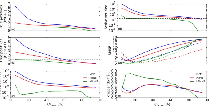
We compare our method to other inverse solvers based on convex sparse priors and show that the thresholding of TF decomposition coefficients in the source space as performed by