Abstract—Progressive refinements of the current sources for the magnetic vector potential finite element formulation are
done with a subproblem method. The sources are first considered via perfect magnetomotive force or Biot-Savart models up to their volume finite element models, from statics to dynamics. Conversions of the common volume sources to surface sources are first done to lighten the computational resources. Accuracy improvements are then efficiently obtained for local currents and fields, and global quantities, i.e. inductances, resistances, Joule losses and forces.
Index Terms— Finite element method, inductor, model refinement, subproblems. I. INTRODUCTION –OBJECTIVES
The current sources in finite element (FE) magnetodynamic problems can generally be considered via Biot-Savart (BS) models, possibly giving the conductors some simplified geometries, with, e.g., filament, circular or rectangular cross sections [1]. The portions of conductors that are slotted into magnetic core regions can first be omitted by considering their interfaces with the cores as perfect magnetic walls, thus neglecting the slot leakage flux. The associated sources are then magnetomotive forces (MMF) [2].
MMF sources are inherently associated with surfaces whereas BS models define source fields (SFs) that are originally volume sources (VSs). It is here proposed to convert the BS SFs into surface sources (SSs) as well, to lighten the computational resources. The developments are performed in the frame of the magnetic vector potential a formulation. Accuracy improvements up to volume FE representations of the conductors, that improve the local field distributions, and from static to dynamic excitations, that accurately render skin and proximity effects, can be done at a second step via the subproblem (SP) method (SPM) [3], [4], that defines a general frame for the whole modeling procedure.
II. PROGRESSIVE MODELS –METHODOLOGY
MMF model – Each slot boundary Γslot, possibly including air gap boundary portions (Fig. 1a), is given an essential boundary condition (BC) that fixes a zero normal trace of the magnetic flux density b. The key is to express this BC with the tangential trace n×a|Γslot (with
b = curl a, n is the unit normal) replaced by the gradient
of a surface scalar potential u, i.e., n×gradu|Γslot, or in
2-D via a floating a on Γslot (constant but unknown) (Fig. 1b) [2]. MMF global sources are weakly associated with all Γslot, as it will be shown in the full paper.
BS model – With the SPM, the BS SF evaluations can
be limited to the material regions Ωm [3], [4], instead of the whole domain with the common method [1]. Such a support reduction already allows to lighten the BS calculations. Then, for accurate combinations with the reaction fields, the BS SFs gain at being projected onto similar function spaces (edge FEs). Also, instead of volume projections of the SFs in the mesh of Ωm, the SFs gain at being calculated there via a FE problem with their boundary values as BCs on ∂Ωm, thus already limiting the BS evaluations to surfaces.
To go one step further, such a preliminary FE problem can be avoided through its inclusion in the main SP. The key is to think of two successive SPs-a-b actually solved together. SP-a first prevents the field to enter Ωm, thus with a reaction field in Ωm opposing the BS field, keeping unchanged the outer field to Ωm (this is simply expressed via both normal and tangential field trace discontinuities through ∂Ωm as SSs; the result is an exactly zero field in Ωm, with no need of volume calculation). Then, SP-b considers the actual physical properties in Ωm, with no more VSs, which is a great advantage. Combining SPs-a-b thus gives a single SP that only requires BS evaluations on ∂Ωm for SSs (Figs. 1c-d). Couplings between MMF and BS models can be defined in 3-D at the interfaces between slots and end winding regions. Additional SPs for volume FE models of the conductors can follow (Figs. 1g-h) [3], [4]. The advantages of the proposed methodology will be shown to be numerous and significant.
X Y Z
(a) total sol.
X Y Z
(b) flux wall sol.
X Y Z (c) BS SF X Y Z (d) sol. w/BS SF X Y Z (e) zoom of (a)
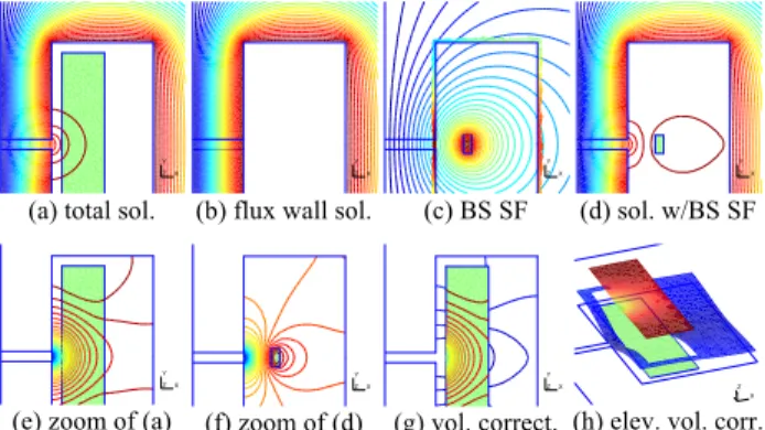
X Y Z (f) zoom of (d) X Y Z (g) vol. correct. Z YX (h) elev. vol. corr. Fig. 1. Current source in a slot with air gap: field lines for (a) full model solution, (b) flux wall solution, (c) BS SF with its projection limited to the core boundary, (d) total solution with BS SF, (e)-(f) window zooms of (a)-(d), (g) volume correction of coil and its surrounding, (h) with its elevation (z-component of a) pointing out the field trace discontinuities.
REFERENCES
[1] P. Ferrouillat, C. Guérin, G. Meunier, B. Ramdane, P. Labie, D. Dupuy, “Computation of Source for Non-Meshed Coils with A–V Formulation Using Edge Elements,” Proceeding of CEFC,
Annecy, May 2014, paper 91.
[2] P. Dular, R. V. Sabariego, M. V. Ferreira da Luz, P. Kuo-Peng, L. Krähenbühl, “Perturbation finite element method for magnetic model refinement of air gaps and leakage fluxes,” IEEE Trans.
Magn., vol. 45, no. 3, pp. 1400–1403, 2009.
[3] P. Dular, L. Krähenbühl, R.V. Sabariego, M. V. Ferreira da Luz, P. Kuo-Peng and C. Geuzaine. “A finite element subproblem method for position change conductor systems”, IEEE Trans.
Magn., vol. 48, no. 2, pp. 403-406, 2012.
[4] P. Dular, V. Péron, R. Perrussel, L. Krähenbühl, C. Geuzaine. “Perfect conductor and impedance boundary condition corrections via a finite element subproblem method,” IEEE Trans. Magn., vol. 50, no. 2, paper 7000504, 4 pp., 2014.
Progressive Models of Current Sources for the
Magnetic Vector Potential Finite Element Formulation
*Patrick Dular,
†Mauricio V. Ferreira da Luz,
†Patrick Kuo-Peng,
†João Pedro Assumpção Bastos and
°Laurent Krähenbühl
*University of Liege, ACE, Belgium †Universidade Federal de Santa Catarina, GRUCAD, Brazil °Univeristé de Lyon, Ampère, France E-mail: [email protected]