The electronic nose as a warning device of the odour emergence in a
compost hall
Jacques Nicolas, Anne-Claude Romain, Catherine Ledent
University of Liège, Department "Environmental Sciences and Management", Avenue de Longwy, 185, 6700 Arlon, Belgium
Abstract:
A self-made electronic nose consisting in a sensor array of six commercial tin oxide gas sensors is used to monitor the odour emission from a compost facility. Supervised data processing tools, such as discriminant analysis, are able to recognize, in real time, the odour of compost with respect to other possible sources in the hall. The paper shows that with unsupervised methods, such as principal component analysis, it is not essential to identify all the possible odour sources during the learning phase. The closeness to the compost group centroid could be used as an indicator of the compost odour level. Alternatively, by a suitable calibration from olfactory measurements, the signals generated by the sensor array can be used to estimate the odour emission rate from the compost hall. Such real time monitoring should allow to assess and to anticipate the annoyance in the surrounding.
Keywords: Electronic nose; Compost odour; Environment; Odour annoyance
1. Introduction
The environmental monitoring is a very promising field of applications for the electronic nose [1]. The objective is to assess the odour annoyance generated by a plant, as an indicator of life quality. This paper discusses the ability of the electronic nose to monitor continuously the emission of the odour generated in a compost hall. The aim is to supply a warning signal to the compost manager when the compost odour is identified and when its level exceeds a given threshold.
The results of the monitoring of the gas emission from a compost pile, using an electronic nose at the outlet of an emission chamber, were already presented [2]. The aim of that specific study was chiefly to provide the manager of the compost facility with a fast method for on-site detection of stress events, like anaerobic conditions in the windrow. The present study concerns the same compost area, but, this time, the electronic nose is placed in the middle of the compost hall and measures the odour in the ambient air. The concerned odour results from the mixing of all the emissions in the compost hall: compost itself, exhaust gas from the machines or neutralising agents. The system must be able to distinguish the compost odour among all those possible sources and to supply a warning signal when it exceeds the annoyance threshold. The monitoring must be carried out at the emission level, but not just above the source. It is more typical of the global odour prevailing in the compost hall and can be used to inform the manager of a possible odour annoyance for the neighbouring.
Some scientific papers concern the monitoring of real-life odours. For instance, Persaud et al. [3] use a hybrid sensor array to continuously monitor the environment of the MIR space station over a 6 months period. The good correlations between the sensor responses and in situ conventional NOx and CO instruments measurements demonstrate the potential of the device in term of sensor performance and selectivity under real operating conditions. The e-nose is also used to monitor the water quality [4] by analyzing the headspace above samples collected in the effluents.
But the monitoring of environmental odours in the field remains challenging. Firstly, the construction of a regression or classification model requires not only the collection of a sufficient amount of observations for the sensor signals but also the determination of the quality of the odour source or information about the odour level. The sensor signals are generated by the electronic nose as an autonomous instrument, but the collection of the additional variables needs the continuous presence of a human operator, during a long period. That is a severe constraint for field measurements, not only during the model construction phase, but still during the further validation and test phases. Secondly, the end user would like to have at his disposal a simple function allowing
him to clearly evaluate the membership of a given observation to a given odour group or to assess the annoyance level, in order to quickly make a decision. Different regression techniques can be proposed to achieve that goal
[5]
. This paper proposes some possible issues to create an "odour annoyance index", if possible, without having to identify all the possible types of odours in the field.
2. Material and methods
The self-made electronic nose consists in a sensor array and a PC board, with a small keyboard and a display. Six commercial metal oxide sensors (Figaro®) are placed in a rectangular 160 cm3 metallic chamber. The sensors were selected on the basis of some operating criteria among the range of sensors proposed by the Japanese manufacturer Figaro and chiefly among the 12 SnO2 sensors used in previous studies [6]. Some sensors
were eliminated for their too low sensitivity towards compost emissions: relative ∆R/R0 resistance variations
near zero caused the removal of two sensors. Two ones were eliminated because of there too long recovery time, their poor stability or their too large signal to noise ratio and an additional one for its redundancy with TGS842. Finally the selected sensors were those for which the contribution to the discrimination power between compost and background air was the highest. When two sensors were available for the same purpose, one from the "800" series and the other one from the "2000" series, this last one was preferred for its low electrical consumption. The six selected sensors are listed in Table 1.
Though TGS2180's response to compost emission was low, this sensor was kept if a signal for humidity correction was needed.
The chamber temperature is kept at 60 C by a heating resistor and natural cooling, thanks to a suitable control system. Relative humidity of the sensor chamber is also recorded. The ambient air is sucked in though a teflon tubing with a flow rate of 200 ml/min thanks to a small pump controlled by the computer code. Data are recorded in the local memory and downloaded in an external computer to be off-line processed by statistical and mathematical tools (Statistica and Matlab). The features considered for the data processing are the normalized raw sensor electrical resistances, without any reference to a base line (or R/ 2
i
R
∑ , where R and Ri are the raw
resistance values) or just the resistances R for the two last figures of the paper.
Table 1: The six selected Figaro sensors and their sensitivity to different vapours
Sensor Sensitivity to vapours
TGS822 Organic solvents (ethanol, benzene, acetone, ...) TGS880 Volatiles vapour from food (alcohols)
TGS842 Natural gas, methane TGS2610 Propane, butane
TGS2620 Hydrogen, alcohols, organic solvents, TGS2180 Water
The compost deposit area of Habay, in Belgium, is studied. It is situated under a shelter. It receives two types of material: either crushed municipal waste, containing an organic fraction, or pure organic waste, resulting from a selective sorting. The aeration is achieved by turning the pile about twice a week. The odour emission from the compost varies with time and with the type of handling. Some trucks or machines also emit exhaust gases and an odour neutralising product is sometimes sprayed in the hall.
During the learning phase, two types of approaches were used.
The first one implies prior identification of the four possible ambiences prevailing in the compost hall: odourless air, compost, neutralizing product or exhaust gas from the engines. Measurements by the sensor array are made either by putting the air intake near the emission source, or by sampling in Tedlar bags and subsequent analysis. For each ambience presentation, all the recorded resistance values, with a sampling rate of 1 record every 3 s, are considered for the model calibration. Hence, this approach favours the learning of the electronic nose with "pure emissions", directly at the source level.
The second approach consists simply in placing the instrument in the middle of the compost hall and to continuously record the sensor signals. The nose of the operator remains close to the air uptake of the instrument and each odour personal feeling as well as all events happening in the compost area are noted, together with the time of their appearance. The resulting file consists in the six sensors resistances facing the type of event for each 3 s observation. It can be used either to validate the model calibrated with pure emissions or to calibrate a new model.
Such monitoring aims at showing the interest of considering as global odour signal the pattern of a sensor array rather than the response of one single sensor. The reason of the rise of the sensor signals may indeed be the compost odour increase, but also the increase of any other gas emission or a sudden change in ambient temperature or humidity. The identification of the cause of the increase of the sensor signal is essential.
Parallel olfactometric measurements are carried out. From time to time, during the electronic nose monitoring, the gaseous emissions of the ambient air is sampled in a 60 l-Tedlar bag placed in a sealed-barrel maintained under negative pressure by a vacuum pump. The bag is directed to the Certech olfactometry laboratory (Seneffe, Belgium) where the odour of the tainted air is evaluated using human panels (standard EN13725). The odour evaluation is made as soon as possible after the sampling.
3. Results
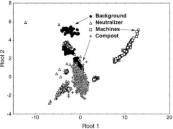
The first approach, considering sequential measurements, may lead to the classification of the observations according to the four identified sources of odour. Such common result is provided by a supervised classifier and requires the identification of all possible sources. That is illustrated in Fig. 1 with the results of a discriminant function analysis (DFA). The figure shows the score plot in the plane of the two first roots of the corresponding canonical analysis: the observations related to the compost odour can be identified as a rather compact cluster.
Fig. 1: DFA visualisation of the four gaseous ambiences prevailing in the compost hall in the plane of the two
first roots.
That analysis considers 2967 observations recorded each 3 s for the different sources: 331 for the background air, far from the different odorous sources, 262 for the neutralizing product, 148 for the exhaust gases from machines and 2226 for the compost emission. Data are non-contiguous in time: the 2967 observations concern several short intervals of time covering a total period of 14 days. A suitable calibration, using ethanol vapour as reference gas, is carried out every day, but no sensor drift is observed for a so short period. The classification of each observation is carried out on the basis of the Mahalanobis distance between the observation and the centroid of each group. The a priori classification probabilities are proportional to the size of the different groups. To validate the classification performance of the model, it was calibrated with only 70% of the observations (chosen at random) and the remaining 30% were set aside for validation purpose. The confusion matrix for those latter observations shows that about 98% of the observations are well classified. A mix-up remains between the background air and the neutralizer, which is sometimes highly diluted in the air.
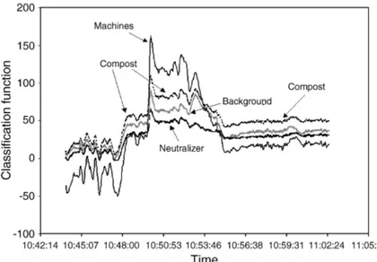
The classification functions supplied by the discriminant analysis procedure were then used as global odour indicators for each of the identified source [7]. The four classification functions are linear combinations of the six features. A case is classified into the group for which it has the highest classification score. Here, the four classification scores are calculated each 3 s for a 20 min period. Fig. 2 shows the evolution of the four classification functions with time where an "odour event" is highlighted.
When observing the evolution of each individual sensor, it was not possible to identify the cause of the odour event. Now, by drawing the evolution of the classification functions, it is showed that the recorded rise of the sensor responses is due to the exhaust gas of a working machine. Before and after that event, the function "compost" get the higher value, but during the event, that is the "machines" function which has the maximum value. That is confirmed by the operator who noted the passing of a working machine near the sensor array.
Fig. 2 : Time evolution of the four classification functions.
Though DFA classification functions may indeed be used as global odour indicators, they lack selectivity. As they are based on the Mahalanobis distances between the observation and the centroid of each group, all the functions are reacting to all "events": only their relative values are of interest to classify observations. Their absolute value is not proportional to the intensity of the specific odour.
Moreover, supervised classification techniques such DFA requires the prior knowledge of all the different odour sources and of the membership of each observation to a given identified group for the calibration data set. Unsupervised analyses, such as principal component analysis (PCA) are often used for visual inspection of the evolution of observations over short time periods [8].
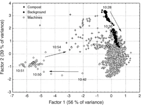
The PCA score plot of 2400 observations recorded every 3 s for 1 day of May is presented in Fig. 3 in the plane of the two first components (explaining 95% of the total variance). When PCA is carried out on the whole data set, the score plot allows highlighting the time evolution of the different odour events.
The "compost" emission constitutes obviously the major group ("+" symbol), but the group identified as the "exhaust gas from machines" is clearly visible on the left part of the diagram. The corresponding points (open circles) follow a path coming from and returning to the main "compost" group. In the same way, the diagram stresses another group, identified as "background" (odourless air), on the upper part (solid circles). However, the separation between "background" and "compost" is not always obvious. That is quite normal: the points identified as "compost" on the upper part of the score plot are those for which the operator noted a "light odour". Such conclusions can be drawn because an observer was present in the compost hall and noted his personal feeling for all events. That is a very hard job which, anyhow, can never lead neither to the identification of all the possible types of gaseous emissions for a given site, nor to the explanation of all the possible causes of the variance.
Fig. 3 : Score plot of a PCA showing the time evolution of different odour events.
Hopefully, the final user does not need to recognize all the possible odours. He wants just to detect the emergence of the compost odour above a given warning threshold.
It should be more relevant to calibrate a PCA model only for those observations corresponding to the source of interest, the compost in this case. Then, by definition, the origin of the factor space should be the centroid of the "compost" group, which represents the core of the observations related to the compost emission. As a result, it is expected that the distance from that centroid could be considered as an indicator of the presence of various gaseous emissions, other than the compost one, no matter their origin. Conversely, the inverse of that distance could be considered as an index of the emergence of the compost odour.
Fig. 4 shows the evolution with time of the inverse of the distance in the 3D space of the 3 first components of a PCA (99.2% of variance). The PC model was developed with the 1637 observations clearly identified as "compost emission" out of the 2400 from the original data set. Next, it is applied to the whole data set.
Fig. 4 : Time evolution of the inverse of the distance to the centroid of the compost group in the space of the
The lower the index is, the more different from the compost emission are the observations. That is obviously the case for various events, identified by the operator by "background air" or "exhaust gas from machines".
The higher the index is, the higher the level of the compost odour should be. That is actually the case for some peak values exceeding the fixed threshold (e.g., 1.5). Nevertheless, several exceeding values cannot be explained by a stronger compost odour. Conversely, the moments when the operator judged that the odour level was important are not always acknowledged by a larger value of the inverse of the distance.
Of course, the reasons of such discrepancies lie in the principle of the PCA itself, which aims at orienting the factors towards the maximum of the variance of the data set. Now, the variance is due to different causes, often the chemical composition of the samples, and not necessarily to the odour level. For example, a previous study [2] conducted with a similar instrument on the same composting facility compared the tin oxide sensor signals to the main chemical compounds identified by GC-MS analyses. Results clearly showed that the sensors are also reacting to less odorant compounds, such as methane, furans or some alcohols.
So, PCA or DFA techniques may lead to construct models identifying qualitatively the odour as a "compost" one, but a regression technique should be used, later on, to supply the user with a quantitative value of the odorous level.
During a previous study related to the same compost odour [9], we used the odour concentration of the samples, as measured by olfactometry, to build a calibration curve for each sensor, relating the resistance variation to the odorous unit per cubic meter.
That study was carried out with 12 sensors in the laboratory on the basis of samples collected in the field. The measurements presented here concern a mobile instrument made of an array of 6 sensors. Though those 6 sensors had the same reference number as 6 out of the 12 sensors from the laboratory instrument, it could be dangerous to extrapolate the former calibration curves to the present application.
However, some spot measurements confirm that, for at least one sensor (TGS822), the previous calibration curve is still valid. So, to illustrate the principle, this calibration curve is used to transform the sensor signal into an odour concentration. The calibration curve is shown in Fig. 5. It links the raw resistance value, R, in kOhms, for TGS822 to the odour concentration C, in ou/m3, by an exponential function of the type:
R = R0- a(1- e-bC),
where R0 , a and b are specific coefficients.
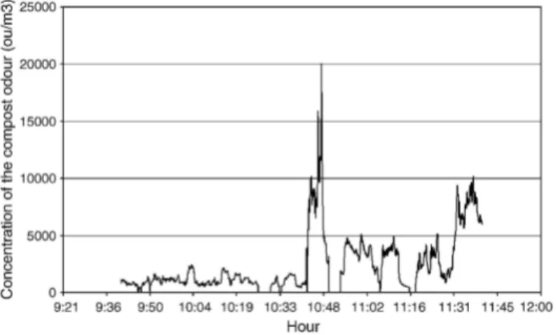
Fig. 6 : Time evolution of the concentration of the compost odour, as calculated by a calibration curve for
TGS822.
Fig. 6 shows the evolution with time of that odour concentration for the same period of May as former figures. It concerns only the emission from the compost, as identified by previous discriminant analysis.
The peak value at 10:48 can be explained by the turning of a compost windrow.
Further comparisons of sensors signals with olfactometric measurements should lead to more sophisticated models to estimate the odour concentration, including all the six sensors responses and using partial least square regression (PLS).
By multiplying the odour concentration (in ou/m3) by the volume air flow emitted by the compost windrow (in m3/s), the odour emission rate in ou/s could be estimated. Previous studies concerning the same compost facility [2] gave us the order of magnitude of the volume air flux for the windrow of 0.004 m3/s per m2 of compost area. Assuming a total area of about 7500 m2 in Habay, the volume air flow should be about 30m3/s, which, for instance, leads to an odour emission rate of 300 000 ou/s when the odour concentration is 10000 ou/m3. That order of magnitude is coherent with other estimations.
Such results, obtained on the basis of the electronic nose, could open many possibilities to monitor and to control compost facilities.
4. Conclusions
The result shows that the electronic nose can be used as a warning device to detect the emergence of the odour of compost. Thanks to appropriate data processing methods it is able both to identify qualitatively the odour of interest (compost) and to estimate quantitatively the odour emission rate from the compost windrows.
For the manager of the compost facility, the next step is to use a simple dispersion model to assess the size and the shape of the odour annoyance zone in real time, from the estimated odour emission rate.
Acknowledgment
The authors are indebted to Certech laboratory (Seneffe-Belgium) for all the olfactory measurements performed on the samples.
References
[1] W. Bourgeois, A.C. Romain, J. Nicolas, R.M. Stuetz, The use of sensor arrays for environmental monitoring: interests and limitations, J. Environ. Monit. 5 (2003) 852-860.
[2] A.C. Romain, M. Kuske, J. Nicolas, Monitoring the odour of compost as a process variable, in: Proc ISOEN'03, Riga, Latvia, June, 2003, pp. 248-251.
[3] K.C. Persaud, A.M. Pisanelli, S. Szyszko, M. Reichl, G. Horner, W. Rakow, H.J. Keding, H. Wessels, A smart gas sensor for monitoring environmental changes in closed systems: results for the MIR space station, Sens. Actuators B: Chem. 55 (1999) 118-126.
[4] H.T. Nagle, R. Gutierrez-Osuna, B.G. Kermani, S.S. Schiffman, in: T.C. Pearce, S.S. Schiffman, H.T. Nagle, J.W. Gardner (Eds.), Handbook of Machine Olfaction: Electronic Nose Technology, Wiley-VCH, Weinheim, 2003, pp. 419-444, Chapter 17: Environmental Monitoring.
[5] J. Nicolas, A.C. Romain, P. André, Choice of a suitable e-nose output variable for the continuous monitoring of an odour in the environment, in: Proc ISOEN2000, Brighton, UK, July, 2000.
[6] A.C. Romain, J. Nicolas, V. Wiertz, J. Maternova, P. André, Use of a simple tin-oxide sensor array to identify five malodours collected in the field, Sens. Actuators B: Chem. 62 (2000) 73-79.
[7] J. Nicolas, A.C. Romain, V. Wiertz, J. Maternova, P. André, Using the classification model of an electronic nose to assign unknown malodours to environmental sources and to monitor them continuously, Sens. Actuators B: Chem. 69 (2000) 366-371.
[8] W Bourgeois, G. Gardey, M. Servieres, R.M. Stuetz, A chemical sensor array based system for protecting wastewater treatment plant, Sens. Actuators B: Chem. 91 (2003) 109-116.
[9] J. Nicolas, A.C. Romain, Assessment of detection thresholds of metal oxide sensors based e-nose to the pollution emitted by odorous sources, in: Proceedings of ISOEN'02, Roma, Italy, October, 2002.
Biographies
Jacques Nicolas is Engineer in Physics. He received his Ph.D. degree in 1977 in Surface Physics in University
of Louvain, Belgium. He joined Fondation Universitaire Luxembourgeoise (FUL, Arlon, Belgium) in 1979, where he worked first on Solar Energy. He is currently the leader of the research group "Environmental Monitoring" in the department "Environmental Sciences and Management" of the University of Liège. He gives lectures in the field of environmental parameter measurement. His main research interest is the development of odour and indoor air pollution detectors usable in the field.
Anne-Claude Romain graduated in chemical sciences from the University of Liège (U1g, Belgium) in 1992.
She received the master in Environmental Sciences from the Fondation Universitaire Luxembourgeoise of Arlon (FUL, Belgium) in 1993. Since 1995, she is a searcher at FUL, which became in 2004 the department "Environmental Sciences and Management" of the University of Liège. She has been working on the development of a malodour detector. Recently, she received her PhD degree on the application of the electronic nose concept to the monitoring of odours in the environment.
Catherine Ledent was an Industrial Engineer student at ISI Gramme (Liège, Belgium). She carried out a work
of end of studies in the research group "Environmental Monitoring" of the University of Liège about the monitoring of the ambient air in a compost hall.