Modeling Radiative Transfer in Heterogeneous 3-D Vegetation Canopies

HAL Id: ird-00405222

https://hal.ird.fr/ird-00405222

Submitted on 20 Jul 2009

HAL is a multi-disciplinary open access archive for the deposit and dissemination of sci-entific research documents, whether they are pub-lished or not. The documents may come from teaching and research institutions in France or abroad, or from public or private research centers.

L’archive ouverte pluridisciplinaire HAL, est destinée au dépôt et à la diffusion de documents scientifiques de niveau recherche, publiés ou non, émanant des établissements d’enseignement et de recherche français ou étrangers, des laboratoires publics ou privés.

Modeling Radiative Transfer in Heterogeneous 3-D

Vegetation Canopies

Jean-Philippe Gastellu-Etchegorry, V. Demarez, V. Pinel, F. Zagolski

To cite this version:

Jean-Philippe Gastellu-Etchegorry, V. Demarez, V. Pinel, F. Zagolski. Modeling Radiative Transfer in Heterogeneous 3-D Vegetation Canopies. Remote Sensing of Environment, Elsevier, 1996, 58, pp.131-156. �ird-00405222�

ELSEVIER

Modeling Radiative Transfer in Heterogeneous

3-D Vegetation Canopies

J. P. Gastellu-Etchegorry,* V. Demarez,* V. Pinel,* and F. Zagolski*

T h e DART (discrete anisotropic radiative transfer) model simulates radiative transfer in heterogeneous 3-D scenes that may comprise different landscape features; i.e., leaves, grass, trunks, water, soil. The scene is divided into a rectangular cell matrix, i.e., building block for simulating larger scenes. Cells are parallelipipedic. Their optical properties are represented by individual scattering phase functions that are directly input into the model or are computed with optical and structural characteristics of elements within the cell. Radiation scattering and propagation are simulated with the exact kernel and discrete ordinate approaches; any set of discrete direction can be selected. In addition to topography and hot spot, leaf specular and first-order polarization mechanisms are modeled. Two major iterative steps are distinguished: 1) Cell illumination with direct sun radiation: Within cell multiple scattering is accurately simulated. 2) Intercep- tion and scattering of previously scattered radiation: At- mospheric radiation, possibly anisotropic, is input at this stage. Multiple scattering is stored as spherical harmonics expansions, for reducing computer memory constraints. The model iterates on step 2, for all cells, and stops with the energetic equilibrium. Two simple accelerating techniques can be used: 1) Gauss Seidel method, i.e., simulation of scattering with radiation already scattered at the iteration stage, and (2) decrease of the spherical harmonics expansion order with the iteration order. More- over, convergence towards the energetic equilibrium is accelerated with an exponential fitting technique. This model predicts the bidirectional reflectance distribution function of 3-19 canopies. Radiation components associ- ated with leaf volume and surface mechanisms are distin-

"Centre d'Etude Spatiale de la Biosphere (UPS / CNRS / CNES), Toulouse, France

Address correspondence to J. P, Gastellu-Etchegorry, Centre d'Etude Spatiale de ia Biosphere, CNES, CNRS-UPS, 18 Avenue Edouard Belin, Bpi 2801, 31401, Toulouse cdx, France.

Received 27 July 1995; revised 21 November 1995. REMOTE SENS. ENVIRON. 58:131-156 (1996) ©Elsevier Science Inc., 1996

655 Avenue of the Americas, New York, NY 10010

guished. It gives also the radiation regime within canopies, for further determination of 3-D photosynthesis rates and primary production. Accurate modeling of multiple scattering within cells, combined with the fact that cells can have different x,y,z dimensions, is well adapted to remote sensing based studies, i.e., scenes with large di- mensions. The model was successfully tested with homoge- neous covers. Preliminary comparisons of simulated re- flectance images with remotely acquired spectral images of a 3-D heterogeneous forest cover stressed the usefulness of the DART model for conducting studies with remotely acquired information. © Elsevier Science Inc., 1996

INTRODUCTION

Modeling the interaction of radiation with terrestrial surface is often a prerequisite for conducting research activities in several scientific domains. Two types of application of interest for environmental studies are mentioned here. The first deals with vegetation studies using remotely acquired information. In many cases, retrieving information from remotely sensed data would benefit of the use of three-dimensional (3-D) models that simulate accurately the spectral behavior of bidirec- tional reflectance distribution functions (BRDF) of Earth's surfaces. This is especially the case where it is intended to assess optical (e.g., albedo) and structural (e.g., leaf area index, LAI) characteristics of ground targets, or more generally where it is expected to associ- ate signal characteristics (e.g., BRDF anisotropy) with some conditions of these targets. As an example, many studies already stressed the spectrally dependent aniso- tropic behavior of vegetation canopies (Kimes et al., 1986). Naturally, this is strongly influenced by the type of cover, the illumination configuration and the spectral domain. For example, Syren (1994) showed that for each degree of decreasing solar zenith angle nadir reflectance factors of pine and spruce forest covers increase by

0034-4257 / 96 / $15.00 SSDI 0034-4257(95)00253-7

132 GasteUu-Etchegorry et al.

1-2%, depending on the spectral domain, the tree spe- cies and the stand age. He observed most important increases with the young pines in the red (3%) and the near-infrared (2.5%) spectral regions. This confirms that in many cases the BRDF anisotropic behavior is a seri- ous constraint for conducting vegetation studies with remote sensing data acquired under different experi- mental conditions, that is, viewing and illumination con- ditions. Associated errors depend on the target charac- teristics and the sun viewing conditions; for example, the albedo of a canopy with an anisotropic BRDF may be underestimated by as much as 45% if it is computed with nadir reflectance only (Kimes and Sellers, 1985). Moreover, the temporal variability of the anisotropy degree of vegetation BRDFs is an additional variable; however, provided that it may be determined with a sufficient accuracy, the latter is indicative of target con- ditions changes. Quantification of vegetation functioning is another important domain of application of radiative transfer models when these are coupled with leaf physio- logical models. Indeed, vegetation development is di- rectly influenced by the within-stand radiation regime and the photosynthesis function of vegetation elements. Various approaches have been developed in the past to model radiative transfer within canopies. They are based on mathematical formulation the complexity of which depends on their objectives, and include empir- ical functions (Walthall et al., 1985), semiempirieal func- tions (Pinty and Ramond, 1986), simulation models with ray tracing, radiosity and Monte Carlo techniques (Borel et al., 1991; Jessel, 1992), geometric models (Li and Strahler, 1986), turbid models with the discrete ordinate method (Myneni et al., 1990; 1991), turbid models based on simplifications of the radiative transfer function (Gao, 1993), and turbid models with approximations of the radiative transfer function of Kubelka and Munk (Suits, 1972; Verhoef, 1984; Gastellu-Etchegorry et al., 1996). Depending on their complexity and on the type of available measurements (i.e., nadir, directional), these models are more or less convenient for retrieving perti- nent information on land surfaces. Generally speaking, the spatial distribution of the target components is a major factor of the BRDF anisotropy. Its influence de- pends on the measurement configurations. Accurate modeling of canopy BRDF requires to take this factor into account.

Three-dimensional leaf canopy transport models such as the K-K model (Kimes and Kirehner, 1982; Kimes, 1991) provide an interesting means for taking into account the architecture of covers. The scene is divided into a rectangular cell matrix, and radiation transport is simulated with the discrete ordinate method; that is, source vectors are restricted to propa- gate in a finite number of directions. However, the K-K model presents some serious drawbacks (Myneni et al.,

1991) due to simplifying assumptions. The most limiting weakness comes from the fact that multiple scattering processes that occur within cells are neglected. More- over, propagation of cell scattered radiation is always simulated from cell centers. These simplifications lead to important errors whenever cells do not have infinites- imal optical depths. This is a very limiting constraint for remote sensing studies where the dimensions of cells must be large enough in order to allow one to work with large scenes. In this context, the hypothesis of cells with equal Cartesian dimensions is another weakness. Indeed, with large scenes the vertical dimension of cells is expected to be smaller than the horizontal cell dimensions; that is, a vertical length unit should be represented by a larger number of cells than the equiva- lent horizontal length unit. Another limitation arises from the hypothesis that discrete directions are equally spaced, which is far from optimal for accuracy and computer time purposes.

With these considerations in mind, we developed a new 3-D radiative transfer model (Gastellu-Etchegorry et al., 1994), hereafter called DART (Discrete Aniso- tropic Radiative Transfer) model. Similarly to the ap- proaches of Kimes and Kirchner (1982) and Myneni et al. (1990), it is based on the discrete ordinate method and on an iterative approach. Moreover, the scene is a rectangular solid made of adjacent cells; that is, it is a cell matrix. The above-mentioned drawbacks are cor- rected. The 3-D radiation regime and the bidirectional reflectance distribution function (BRDF) of 3-D cano- pies are realistically simulated through the consideration of topography, major physical mechanisms such as the hot spot effect and leaf specular reflectance, and four types of scatterers (i.e., leaves and grass, soils, water, and trunks). Moreover, this model is aimed to allow one to distinguish the radiation components associated and not associated with leaf mesophyll information.

This article focuses on the mathematical description of the model. After a brief presentation of the scene modeling, the simulation of directional transport and the major steps of the iterative approach are described in the third section. This is followed by a full description of within cell scattering mechanisms. The emphasis is laid on single and multiple scattering mechanisms within leaf cells; scattering mechanisms that arise from other cell types are also described. Cell interactions are sys- tematically analyzed by considering total scattered radi- ation, scattered radiation not associated with mesophyll information and first-order polarized scattered radiation. Two simple accelerating techniques for reducing com- puter memory constraints and computation times are described in the fifth section. Finally, a preliminary comparison between DART simulations and remotely acquired spectral images of a tree canopy is presented in the last section.

Radiative Transfer of Heterogeneous Vegetation Canopies

133

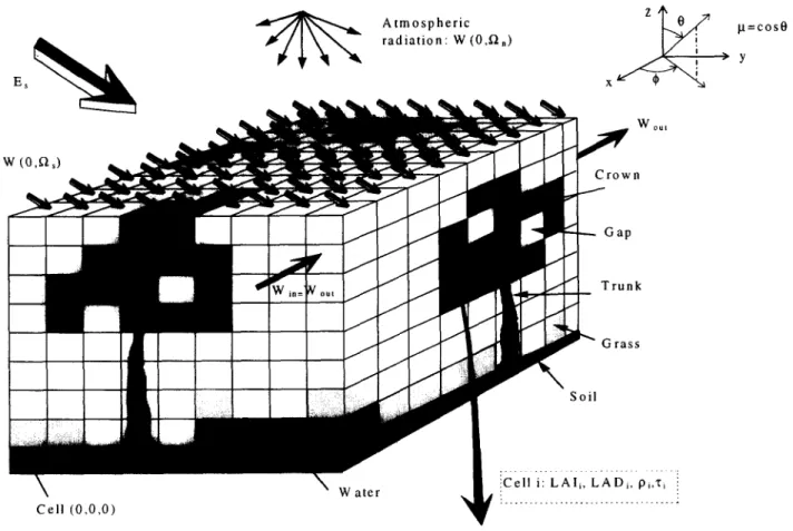
Es Atmospheric Z ~ H =cos0 radiation: W(0.f~,) i i > Y I X

Figure i. Representation of a cell matrix and its general illumination.

SCENE MODELING

The DART model does not require that the individual cells that constitute the 3-D scene have necessarily equal dimensions (Ax, Ay, Az) along the Ox, Oy, and Oz axes. So, the numbers of cells along the vertical and horizontal axes can be independent, which results in important reductions in computer memory require- ments and computation times. This is especially interest- ing for simulating the radiation regime of large scenes where the vertical variability is larger than the horizontal variability. Naturally, the selection of unequal dimen- sions along Ox, Oy, and Oz axes modifies the direction cosine values of the propagation directions.

Individual cells (Fig. 1) are identified with the x, y, and z coordinates of their centers. Lower (upper) cells of the scene have an altitude level z--0 (z = H). The total number of cells is 1= (AX" AY" AZ) / (Ax- Ay. Az), where AX, AY, and AZ are the Cartesian dimensions of the scene. Cells are used for simulating different types of scene elements, that is, leaves, soil surface, grass, water, and trunks. Depending on their informa- tion content, cells are simulated as turbid media, with volume interaction mechanisms, or solid media with surface and possibly volume interaction mechanisms. Cells characterized by different optical behaviors are

said to belong to different types of cell. Two approaches can be used to specify the optical properties of each individual cell:

• Cell type j, with je [1 J], and specific optical and structural characteristics of the elements within the cell; for example, with leaf or grass cells, hereafter simply called leaf cells, these characteristics are the LAI, LAD (leaf angle dis- tribution), and foliar reflectance and transmit- tance. In a first step, before tracking radiation propagation, the DART model uses these input parameters in order to compute the scattering transfer functions T(j, fLf~') that characterize cell volume scattering mechanisms of all j cell types; Q and t~' are the incident and scattered directions, respectively. Leaf transmission func- tions T(j,fl) associated with a unit leaf area vol- ume density and a unit propagation length are also computed for handling leaf cell interaction mechanisms.

• Cell type j, with j e [1 jr]. This index indicates the relevant volume scattering transfer function T(j,t),~'). In the case of leaf cells, this index is input with the leaf cell area index. So, the in- dex j indicates also the relevant cell transmis-

134

Gastellu-Etchegorry et al.

sion function T0,t) ). These discretized func- tions may come from measurements, analytical computations or simulations conducted at finer spatial resolutions.

The information content of any cell is specific to that cell and is a constant for the whole cell. If necessary, the operator can easily add other types of elements, provided that he knows either their optical and struc- tural characteristics or their transmission and scattering phase functions.

The K-K approach is adopted for dealing with scene boundary interactions. It is assumed that the whole scene can be considered as the juxtaposition of identical cell matrices. The hypothesis relies on symmetric con- siderations. So, the above-mentioned cell matrix is a simple building block that when replicated will simulate the entire scene. With the assumption that all neighbor cell matrices have identical optical behaviors, it results that as a source vector escapes the sides of the modeled cell matrix, there is an equivalent source vector escaping an adjacent cell matrix which enters the modeled cell matrix at a symmetric position. It means that the radio- metric behavior of the entire scene can be simulated with the simulation of an individual cell matrix. The dimension of this cell matrix depends only on the basic unit of structural repetition within the scene; for exam- ple, it is smaller for homogeneous tree plantations than for disturbed dense forests (Kimes, 1991).

REPRESENTATION OF THE DIRECTIONAL TRANSPORT

Discretizafion of the Propagation Directions

The DART model relies on the discrete ordinate method; that is, the angular dependence in the transport equation is approximated by discretizing the angular variable t) into a number N of discrete directions t),, with ne [1 N]. These directions are the only possible directions of incident and scattered radiant fluxes. They are not necessarily equally spaced and can be selected a pr/or/by the operator. The total number of discrete directions is

v ,~(u) N = ~ ,

u = l v = l

where u is the discretizing level of coordinate/~, that is the cosine of zenith angle 0, and v is the discretizing level of coordinate ~, that is, the azimuth angle. A negative/J indicates a downward direction, and a posi- tive/t indicates an upward direction. Thus, for a zenith level u we have

v(u)

azimuth levels. It means that the azimuth angles

~(u,v) and q~(u',v)

may be different if the indices u and u' are different.

Discrete directions are associated with a number of contiguous sectors A ~ defined by their azimuth Acp~

and zenith A0n angle intervals. The solid angle of each sector is

At),,= I I Idul.d~p with,u-- cos o

A~n AOn Moreover, we have

N

£ A ~ . = 4n with ([1.) = (0~,~0v(O~)). n = l

The DART model starts with the determination of all cells encountered by any source vector that propagates in the scene 1) from the center of cell (0,0,0), and 2) from the center of each face of cell (0,0,0) for all N discrete directions ( ~ ) . Indeed, geometric propagation of radiation is always simulated from cell centers or cell faces. This leads to the building up of seven look-up tables. For each cell i encountered the within cell propa- gation length Ali and the coordinates of the entrance point are systematically computed and stored for further processing. These look-up tables eliminate unnecessary repetitive computations during the tracking of source vectors. Thus, during the procedure that tracks radiation propagation, the coordinates of the ith cell encountered by a source vector that propagates within the scene are the coordinates of the cell where it originates plus the ith coordinates of the look-up table.

Radiation Transport

The general transfer equation of steady state monochro- matic specific intensity

I(r, fl)

at a position r and along a direction ~ (Hapke, 1993) is

o

- a ( r , O ) . I(r,O) +

O3"dn'.

(1)

gt, r/, and ~ are directional cosines with respect to the z, y, and x axes,

a(r,f~)

is the extinction coefficient, and

ad(r, tT~t~)

is the differential scattering coefficient for

photon scattering from direction (t)~ into a unit-solid angle about direction (~).

Assuming that we represent the N discrete direc- tions by (t),), with ne [1 N], and that we distinguish the first and multiple collision terms, the angle discretized transport in 3-D Cartesian geometry along the (f/0) direction is

Iu,j'd+ rlo'~y+

,0" d]I(r,f/0) ffi

- a(r,g),j)'I(r,~j) +

Q(r,~¢) + ~] E

C,~'ad(r,t~'~j) "I(r,t'~),

u ~ l v - 1

(2)

where u and v are the discretizing levels of coordinates /~ and ~0, respectively. Indices i and u belong to the interval [1 U], and indicesj and v belong to the interval [1 v(u)]. Cu~ represents the weight associated with the

Radiative Transfer of Heterogeneous Vegetation Canopies ] 3 5

direction (t'~) in the scattering mechanism

(fLv~)

where the incident radiation along the direction (t'~) is scattered towards the direction (f~0). Q(r,~j) is the first collision source.

I(r,t~) may represent either the mean specific in- tensity, that is,

1 • J~aaS(r'D)'dD

in the angular sector A~uv or simply the exact specific intensity along the direction (t'~). It depends on the definition of the differential scattering coefficients aa (r,t~uo--~f~0); that is, if they stand for mean values associ- ated with scattering mechanisms from the angular sector Af~,v towards the angular sector AD 0, or if they stand for values associated with the scattering mechanism from direction f~,, towards direction fl0. Of course, the values of weights C,o differ depending on the meaning of the differential scattering coefficients. These weights must be chosen in order to satisfy symmetry and balance conditions (Myneni et al., 1991).

If I(r,f~) and ae(r,f~'-~) are mean values, and provided that the angular sectors Af~,~ are sufficiently small and that the scattered radiation is not too aniso- tropic, then weights C,v are simply assumed to be equal to Af2~v. On the other hand, if I(r,t~,~) stands for the exact specific intensity along the direction (~,o), the values of C,~ depend on the quadrature approach that is used to compute the integral of (1). In theory, the Gauss-Legendre quadrature is the most efficient ap- proach, It leads to an approximation whose order is, essentially, twice that of Newton-Cotes formulas with the same number of evaluations of the specific intensity l(r, D0). Naturally, high order of approximation is not the same as high accuracy. High-order translates to high accuracy only when the integrand is very smooth, in the sense of being well approximated by a polynomial (Press et al., 1992). Although the Gauss-Legendre quad- rature approach is very general and simple, it has limita- tions. For example, with strongly anisotropic situations, it may be necessary to use an asymmetric set of Gauss- Legendre directions with several directions around the anisotropy or the anisotropies, which requires an a pr/or/knowledge of the directional distribution of the anisotropies. A second and more serious weakness, called ray effect, arises in the case of 2-D and 3-D geometry. This is due to a defect in the discrete ordi- nates formulation itself. Indeed, according to the discret- ized radiative equations, scattered radiation can stream only along preset directions (~,), which may imply that the influence of some isolated point sources, scatterers, and absorbers within the scene is totally ignored. The choice of equally spaced discrete directions tends to decrease the probability of ray effects. Finally, in the context of remote sensing studies, another limitation of the Gauss-Legendre quadrature originates from the fact

that we usually require higher accuracy for directions close to the upward vertical (i.e., directions that are associated with viewing configurations from space) than for downward directions. As a result, it may be better to tailor an angular discretization scheme that is finer for upward directions close to the vertical.

In fact, as already mentioned, the DART model works with any input set of discrete directions (e.g., Gauss-Legendre directions or unevenly spaced direc- tions). Functions that characterize cell interaction mechanisms, e.g., the scattering transfer functions and transmission functions of leaf cells, are determined with the so-called exact kernel method (Myneni et al., 1991). An example of computation of these functions is shown below in the following section. It follows that the dis- crete radiative transfer equation is simply:

0"~zz + t?0" ~yy + ~,j" ~xx W(r, a0) = - a(r,f~,j). W(r,f~0) + Q(r,t~0)" Aft0

v o(u)

+ Z Z a,(r,t~,v-*O~j)" Af~ o" W(r,f~,v), (3) u = l v = l

where W(r,f~uv) and W(r,f~0) are quantities that are proportional to the terms I(r,f~v)'AD~v and I(r,f~o). A ~ 0, respectively.

The physical quantity W(r,~u~) represents the flux of energy along the direction ( t ~ ) in a cone (A~,o) at a position r. It can be envisioned as a flux of photons that stream through a cylinder of infinitesimal section AS (AS < < Ax-Ay, Ax-Az and Ay" Az) and the axis of which is parallel to the direction (f~u~). It has the dimen- sion of a power (W).

W(r,~uv) = Las(r,~,o)" A~,~'AS,

where Las(r, Ouv) is the radiance of the surface AS normal to the propagation direction (t~). We define the term "specific intensity associated with the flux W(r,D~)" with

I ( r , ~ ) = W(r,t~) within a surface unit normal to the A ~ propagation direction (t'~),

I(r,O,o) = o outside the above-mentioned surface unit.

Direct Sun Radiation and Anisotropic Atmosphere

The DART model was designed in order to handle both direct sun radiance and downward atmospheric radiance that may not be isotropic. Actually, the sky radiance distribution is often very anisotropic (Dave, 1978). Moreover, it ranges from 5% to 40% of the total down- ward radiance, under usual atmospheric conditions. Thus, total irradiance incident on a scene has two com- ponents: the direct sun and atmospheric source vectors. They are assumed to originate from a fictitious cell layer at the top of the scene. Direct sun source vectors (Fig.

136

GasteUu-Etehegorry et al.

1) propagate along the direction (f~s). At the top of the scene their value is

w(t)~) -- EAt),). I~,1" Ax.A v,

and the atmospheric source vectors are

w,(t),) = L~(~). lU, I" Ax. Ay. At)~,

where E,(t),) is the sun constant at the top of the scene, t), denotes the solar incident direction, and L~(t),) is the atmospheric specific intensity along direction (ft,), with ne [1 N'], where N' is the number of downward discrete directions. Anisotropic atmospheric conditions are simulated with the use of an anisotropic distribution La

(t)n)

that is specified by the operator. Different analyt- ical expressions are available in the literature (Per- raudeau, 1988). They depend on local sky conditions, that is, clear sky or cloudy sky. Three major approaches are generally followed for describing the angular distri- bution of the sky radiance (Liang and Stralher, 1993): 1) numerical solutions of the radiative transfer equation, 2) analytical approximations of the radiative equation, using for instance an Eddington-type approximation or a two stream approximation for the multiple scattering component, and 3) statistical techniques to fit collected sky radiance.

Thus, total downward irradiance of an upper cell is

Hereafter, a source vector, along direction (f~,) with nE [1 N], incident on cell i, with i¢ [1 I] is noted W(0,t),). The associated transmitted source vector, after a propagation length Al~ in cell i is noted W(Ali, D,).

The Iterative Approach

The model processes the interactions of each individual source vector with all encountered cells as it propagates down and up in the scene (Fig. 2). During their propaga- tion source vectors meet individual cells. Interaction mechanisms depend on the cell type, that is, the ele- ments (leaves, soil, grass, water, trunk) within these cells and their associated structural and optical properties. Source vectors are transmitted through gaps, totally intercepted by opaque cells (e.g., soil and water cells), or partly intercepted and transmitted by semiopaque cells (e.g., trunk, leaf, and grass cells). Radiation inter- cepted by a cell gives rise to scattering and absorption mechanisms. Thus, each cell where scattering mecha- nisms take place becomes a secondary source.

In a first iteration all direct solar source vectors are processed. They give rise to secondary source vectors in all illuminated cells that are characterized by non-nil scattering phase functions. A solar source vector is pro- cessed until it reaches a zero threshold value T1 or

Iteration:

order k

Figure 2.

I Cell matrix and parameters

1

4 Sun radiation (E,,D~)

I DIRECT

SUN ILLUMINATION

I

AND 1 ST ORDER SCATI'ERING

~ ,I Atmospheric radiation (wa,D~)

I

I MOLT ' OROERSCA R O I

Energy stored as Cim coefficients I

ENERGY STATUS PER CELL SCENE BRDF DIRECTIONAL IMAGE SIMULATION

Schematic structure of the DART model.

encounters a medium where it is totally absorbed and scattered. This zero threshold value is selected by the operator; it is expected to be proportional to the inci- dent irradiance multiplied by the relative error that is tolerated.

In a second iteration all source vectors that originate from all secondary sources, and the atmospheric source vectors, are processed. These give rise to tertiary source vectors that are further processed in a third iteration. Iterations are systematically conducted for all sources and for all N directions. Radiation that escapes from the upper cells of the scene is stored at each iteration. Processing goes on until source vectors escape from the canopy or reach a zero threshold level of flux within the scene. This threshold value is the product of an operator specified factor T2 divided by 4n, and multiplied by the mean hemispherical flux < ~W> 1,~ and by the solid angle AD, of the cone of propagation. The term < ~W)1.2 is the maximum value of the mean cumu- lated fluxes < ~ W > that exit cells in the first and second iterations. The quantities ( ~ W ) are computed during the illumination phases as the product of the cell single scattering albedos by the energy intercepted by the cells. Thus, Ta'<~W)l~/4n is an intensity threshold. All source vectors W(t)n) that propagate across the scene such that

At),

w(t)n) < T~" < ~W>I,~"

4n

are eliminated. Figure 3 shows the cumulated sums of cell scattered source vectors in iterations 1-8, in the ease of an homogeneous foliar canopy (LAI = 2, spheri- cal LAD, mle~ = 0.9, Psoa = 0) with a direct sun illumina- tion (SKYL -- 0). The horizontal axis stands for the values of source vectors. All intensity values are divided by the

Radiative Transfer of Heterogeneous Vegetation Canopies

13 7

EW

0.9

L'WI 0.8 0.7 0.6 0.5

0.4

Figure 3. Cumulated sums of cell scattered

0.3

source vectors in iterations 1-8 plotted against source vector intensity. Values are divided by o.2 the total energy scattered in the first iteration.

_0.1

They were obtained with an homogeneous leaf canopy ( L A I = 2, spherical LAD, £01eaf = 0.9, o

Psoii = 0) and a direct sun illumination (SKYL = 0).

Iteration I

Iteration~ 2

/

Iter~on3 /

/

Iteration 4 f

- / /

/

/ Iteration 5 Iteration

6 Iteration

7 Iteration

8

r , / , . / W

20

40

60

80

100

120

140

160 10 .6

total energy scattered in the first iteration. Thus, the

cumulated sum of the first iteration tends towards one, whereas asymptotic values in iterations 2-8 are 0.47, 0.25, 0.14, 0.07, 0.039, 0.021, and 0.011, respectively. The standard deviation of scattered source vectors strongly decreases with the iteration order; that is, the upper and lower cells tend to scatter the same energy at large iteration orders. Moreover, the larger intensity levels associated with iteration n tend to be systemati- cally smaller than those associated with iteration orders smaller than n. So, the selection of a threshold intensity level equal to the mean source vector scattered at itera- tion n leads to the elimination of 1) all source vectors scattered at further iterations and 2) all source vectors that originate from iteration orders smaller or equal to n and that reach this threshold value after some propagation within the scene.

With clear sky conditions the intensity threshold value is selected with iteration one only because the mean scattered flux is larger for iteration 1 than for iteration 2. However, with very cloudy conditions, that is, conditions that are not appropriate for remote sensing acquisitions, this may not be true. This explains why iteration 2 is considered in addition of iteration 1. In that case, the model is not aimed to simulate remote sensing acquisitions but to simulate 3-D radiative trans- fer only, for example, for further modeling of canopy photosynthetic activity. The modulation of the threshold value by Af~n is aimed to retain an acceptable accuracy along narrow anisotropic directions such as those associ- ated with the hot spot configuration (i.e., equal illumina- tion and viewing directions).

Scene Bidirectional Reflectance Factors

Once all source vectors have been processed, directional reflectance factors of all upper cells are computed. The energy flux that escapes an upper ceil along direction ( ~ ) being Wout(Z = H,~v), the associated reflectance fac- tor is

a ( o o ) =

n" Wout(z = H, Ov) 1

!~o " Af~v _{W,(z = H,f~,) + ~ Wa(z = H,n,)'} n f f i l

where

(4)

( ~ ) = viewing direction with zenith and azimuth angles 0o and ~0v,

/Iv = cos Ov,

= total irradiance of an upper cell,

1 Wout (z = H,F~o) Ax" Ay /Iv" A~o

= radiance of an upper cell along the direction (f~v).

In the absence of atmospheric radiation, the upper cell bidirectional reflectance factor is

n" Wout(z = n,t%) W,(z = H,t~,)"go" At~"

In a further stage the BRDF of each upper cell is resampled in a cylindrical coordinates system for ob- taining a cylindrical representation of the BRDF. De- pending on the choice of the operator, different types of results can be finally obtained. For example, if the position, viewing direction, and instantaneous field of view of the airborne or satellite sensor are known, the DART model simulates the remote acquisition of spectral images.

WITHIN C E L L INTERACTIONS

W h e n a source vector encounters a non empty cell, that is, a cell with some information content, the model handles interactions with the help of the cell optical

138

Gastdlu-Etchegorry et al.

properties. Procedures used to simulate radiation inter- actions within cells depend directly on the cell type. For example, the simulation of scattering mechanisms within leaf cells relies on the use of scattering T(j,~,f2) and transmission TOg, O ) functions, which is not the case with soil cells. As already mentioned, cell optical charac- teristics are either input parameters, or are computed in the first step of the DART simulation, with the optical and structural properties of the elements within the cell. An example of computation of leaf scattering and transmission functions is first examined. Handling other cells is globally similar. It is presented in a further section.

Leaf Cell Transmission

Leaf cells are treated as turbid media, with leaves as- sumed to be small plane surfaces with leaf scattering phase functions

f(j,~f,O;'*f2o),

where j indicates the cell type and (f2f) is the leaf normal orientation. The cell leaf area density is

uf.

Leaf normals can have any possible orientation. They are defined independently of the N discrete directions of propagation. Their angular distri- bution is represented by the normalized leaf angle distri- bution function grog,~s)/2n. Leaf cell dimensions must be such that enough leaf area is contained therein, upon which the use of local phytometric attributes such as gfog, f~f) would be meaningless. Natural vegetation clumping tends to ensure the validity of this hypothesis. Thus, the transmission factor (Fig. 3) associated with a radiation that propagates along a direction (f~,) through a foliar cell i of cell type j is

T(AI,,~,)

= exp[ -

Gog,~n)'ut(i)'Ali],

where

('2n

f l

cog, a . )

is the mean projection of a unit foliage area in cell i on a surface unit perpendicular to direction (£~,). Ali is the total pathlength through cell i along direction (f~,). We call Tog, t'& ) the discretized J x N matrices T(j,O,)= exp [ - G(j,O,)] with j e [1 f ] and ne [1 N], where J' is the number of leaf cell types. Thus, we have

T ( A / i , n n ) =

[T(j, nn)]Ufl O'ati.

Consequently, with a flux W,. (0,t3~) incident on cell i along the direction (O,) the transmitted flux that escapes cell i along the direction (O,) is

Wo,,t(AI,,~.) = T(A/i,O.). W~.(0,~.). (5) It results that the source vector intercepted along the path (Ali,£~,) is

Wi.,(A/,,O,) = [1 -

T(AIi,n,)I.W,.(O,O,).

(6)

Scattering Transfer Functions of Leaf Cells

The propagation (Fig. 4) of a source vector W(I,f2,) throughout a cell i along a direction O~, where le [0, A/i] is the pathlength from the entrance point (A) of cell i, gives rise to scattered source vectors ~ (A/i,OT"f~) along the directions (O~, At3~), ve [1 N]. The type of cell i being j, we have

~(Ali,~,"*~)=Iaa~Iatil'2W(l,f~,)'uf(i)"

I ~," " " I " gf(j'f2f)~s 2n

•fog, f~f,g~,-*Ov)'dt3f" dl"

df~ = Win(0,~'~s)" [1 --

T(Ali,O,)]

" I,d lf , f sl ' Os, O;-'Ov)" dt s" dt v

Wint( Ali, fls)

= s)

.fog, Of, t2;-*O~), dt2f. dO,,

wherefog, O;'*~v, Of)

is the leaf scattering phase function. The total specific intensity ~AI~,F~,'-*~) associated with the flux ;¢~(A/i,t~,--*f~°) is

,£ (A/,,t3;-*n~) = i(0,n,). An,. [1 -

r(Al,,a,)]

G(j,n,,)

" I~ lf~,' asl " ~f(j,t~s,n,--'qd

d~s.

With small angular sectors the cumulated scattered flux

to direction f~, is

~l(A/i,O,--~v) W~"t(Ali'O') I

~f)

= cog, as)

•fog, P.s,O;-*t2~).df~f

Ao~, = W,n(O,a,)'[1 -- r(al,,Os)].r(j,o,,Oo),

(7) where Wi, (0,~,) is the value of the source vector, along direction (t~,), at the entrance of cell i, and TOg, D~,D.v) is the cell transfer function. This is discretized as a N× N scattering transfer matrix the terms of which are equal to

I gs(J't~f)" Lf2s" f~s] "f(J,ns, t~'-*~v)'dOs

f _2n

[T(j,t'~,,n~)] = ~ -J2~

dn~

Jz~n~

G(j,t~)

Scattering transfer matrices [T(j,O,,O~)] are precom- puted in order to minimize repetitive computations. Each scattering transfer matrix [T(j,E~,,~,)] is broken up into two matrices that are assumed to be dependent

[Ta(j,~s, Ov)]

and independent [T,,Og,O,,t2~)] of leaf meso- phyll information. These scattering transfer matrices may be anisotropic and rotationally variant. They can be derived from radiometric measurements or from computations based on whatever method is selected; for example, with the usual assumption under which

Radiative Transfer of Heterogeneous Vegetation Canopies 139

Figure 4. Within cell single and multi- ple scattering mechanisms.

w(o,t~) A W l ( A l i , ~ . s - - ~ ) = 7/~(Ali,D.~).exp[-G(i,~,v).uf(i).zSsi(K~) ]

/

B W(O,f~).T(~,~) WM(AIi,~--K~) IIABII=AI~(D.0 IIAM~II=Aq(t~) IIM~DII=As~(D,.,,)

the leaf scattering phase function f(j, ay, t~,--,a~) is the sum of a lambertian component fa(j, af, a,--,f~) and a specular component fgj, ay, f~,~tq~). Examples offd(j,f]f, fl,~t'l~) and fi(j,f~f,f~,~ao) functions are shown below. Then, the transfer function is the sum of two matrices associated with lambertian and specular components. The lambertian component, also called diffuse foliar component, is usually assumed to be due to radiation that penetrates the leaf to be absorbed by leaf metabolic constituents and to be multiply scattered at the leaf dielectric interfaces. This is randomly polarized and carries information about the leaf interior. On the other hand, the specular component is usually associated with radiation that does not penetrate the leaf and that is reflected by leaf surface; it does not contain information about the leaf mesophyll. Specularly reflected radiation is often assumed to be linearly polarized (Egan, 1985). It may represent an important proportion of total reflec- tion; for example, 30%, 17%, and 2% of the total light reflected in the green (550 nm), red (630 nm), and near-infrared (790 nm) spectral regions, respectively, by a soybean canopy in the incidence plane at 30 ° view zenith angle with a - 3 0 ° sun zenith angle (Rondeau and Herman, 1991).

Source vectors associated with leaf lambertian scat- tering, that is, photons having undergone at least one leaf volume scattering are noted Wdf(~). Conversely, source vectors not associated with any leaf volume scat- tering are noted W,y(f~). Polarized source vectors are noted W,(a). Thus, source vectors are three dimension vectors:

[w(a), w~(~), w~(~)] with w(a) = w~(a) + w.~(~).

Proportions of leaf scattered radiation that arise from volume, surface, and polarization mechanisms are noted df(a), nf(a), and p(a), respectively, Thus, we have Way(a) = gila), w(f]), w,y(a) = nf(t~). W(a), W,(f]) = p(a)- W(f~), df(O) + nf(t~) = 1.

Thus, an unpolarized sun radiation incident on the scene is noted [W(a),W(fl),0].

Leaf Specular Reflection

According to Vanderbilt et al. (1991), leaf specular phase functionsfi(j, ay, a,---~) are assumed to depend on three parameters: the angle Wf, between the incident radiation (a~) and the leaf normal (fif), the surface refraction index nj (-~ 1.5), and a parameter Kj(x,CgZ,), between 0 and 1, that characterizes the smoothness of leaf cuticle:

f,(j, as, ar--oo) = tqx,%,), e~(nj,%) .,~(~,a*),

where d~(ao,A*) is a Dirac function; that is, d~(t%,~*) = 0 if a~ differs from the specular direction f~*. This is a function of incident direction (fl,) and leaf normal (f~s). R~(n~,~y,) is the Fresnel reflectance averaged over the polarization states:

RZ, n ~ , 1 [sin2(qJf,- 0) tan2(Wy,- 0)] "( ~' f~) = 2" [sin~(~f • + 0) + tan2(~f • + 0)'l

sin 0 = sin Wy, nj The polarized component is

R2, ~ , 1 Fsin~(~fs - 0) Ptn~ Y~/= 2" [sin2(Wy, + 0) -

tanZ(Wy, - tan2(~f, + ~]" Hereafter, polarization mechanisms are simulated in a very simple way: The polarization of incident radiation is not taken into account, and single scattering mecha- nisms are assumed to be the only mechanisms that give rise to polarization.

The specular flux ~K~(A/~,f~,--}av) and the polarized flux ~(A~.,f~,-"f~v) scattered along the direction (ao), due to an intercepted flux Wi,t(A/i,f~,) are

~K(A/,,[I,~) = T,(j,a,,av).Wi.t(AL.,a,) and

140

Gastellu-Etchegorry et al.

with

"O*

In,. oj*l.gr(J'

~ ). &(x,%) . R~(n> % )

r,(j,n,,nv)--

2~

.An?,

G0,n,)

I0,. 071. *(J'n?). N(x,%) • R~(nj,%) 2n

r,(j,n,,no) ~

• a n ? .

c~j,n,)

The term AOf represents the solid angle that comprises all leaf normal directions that satisfy the conditions of specularity for the reflection (O,,An,) --" (Or,An0:

n , . n s = - no.o~ and

r f t - a c o s ( n , . n o ) = 2 . a cos(n~.nf) i f o , . o f < o , - a c o s ( O , . n v ) = - 2 . a cos(O~.nf) i f n , . O / > 0 . According to Reyna and Badhwar (1985), the leaf normal

" 0",~o *"

direction n ? = t 7 7) that induces the specular reflec- tion (n;--n~) is defined by

cos 07 = Icos 0 , - c o s 0~1 and 42(1 - 0,. 0o)

tan (o*

41

- c o s 2 0," s i n ( 0 , - ~/1 - c o s e 0v" s i n ~a~

= ~/1 - cos ~ 0/cos (a, - 41 - cos ~ 0o" cos ~" Moreover, the angular cone of leaf normals that leads to the specular reflection is

2

An? = 4.1o,.nsl (Vanderbilt et al., 1991).

For first-order scattering mechanisms associated with di- rect sun radiation, incident radiation is assumed to be monodirectional (i.e., An, ~-, 0). So, An~ ~ AOo/(4.1 n,. n j I). Then,

" 0 "

;yf/ss(A/,,n;..}nv ) = Wint(al," as).gr(j, ;f )

GO, o,)

8,~

* 2 ILl/* .K~(x,ue~).lt,(n>

s,)" AO~,

" O *

~(a/,,fl,---Ov) = w, ot(a/,, o 0.go(j, ~ )

c(j,o,)

8rt

.t~j(~,'I'~) . i%(nj,'I'~)" Any. ~ *

Leaf Lambertian Scattering

The lambertian behavior of leaf elements is modeled with the leaf hemispherical reflectance pa,l~f and trans- mittance zd,l,a coefficients:

fa(j,n;-'P.o, Oy) =

~'P~,'e~,~S,)"

los. n J,

(n,. os).(as, oo) < 0,

1. r,,,o~d,%)" Ias, aol, (n.. as). (as- an) < 0.

Use of this leaf scattering function in the general expres-

sion of the cell transfer function leads to the leaf cell diffuse transfer function [Tdj,O,,Ov)].

Within Cell Single Scattering

Total within cell single scattering in the 4n space, due to an incident flux w(o,n,), is

~¢f(A/,,f~) = I4 J(A/,,f~;--t~v) • df~v N

-- E[~l(Al,,t~;--O d +~(A/,,f~;--t~o)], ve[1 N], v = l

where gC~I(A/i,O,--}Oo) and ~ (A/i,O,oD.o) are the single scattered source vectors associated with the scattering transfer functions Te(j,n,,oo) and L(j,n,,oo).

In fact, the flux YJi((A/~,O,~Oo) undergoes further inception and scattering before escaping the cell. Trans- mission along (nv) within the cell is computed with the assumption that the scattered flux ~g"(A/,n,oov) originates from a unique point, called middle point (Ms), within the cell i, and not from the cell center. Simulation of scattering mechanisms from (M,) instead of the cell center leads to more accurate results, especially for cells with large

uf

values and for oblique propagation directions. In a second step, the geometrical propagation of scattered radiation that has already gone out of the cell is simulated from the cell center. The point (M,) is defined as the point along the path (A/,n,) such that 50% of the total intercepted radiation Wi.t(A/~,Os) is intercepted before this point. The pathlength between (M,) and the entrance point of cell i is called Ar~. We have

f4J(Ar,,O;-'Oo,'dO~=I"I4~AI,,O;-}I2~)'dOv

Ar~ -- In 2 - In[1 + exp( -

uf(i)" GO, O, ) •

AI,)]

(8)

,t(i). c(j,o,)

The scattered radiation Wx(A/,n,--}O~) that escapes cell i along (n~) corresponds to the attenuation of ~ ( A l , fl;-}Oo) within cell i after a propagation length As~(n~) from the m i d d l e point (M,). It is a single- scattering radiation:

W~(Al,,fl;--n 0 = ;Nl(Al,,fl,~n~)

• exp[ -

G(j, flo).uy(i).As,(no].

This term is the sum of a diffuse and a specular compo- nent:

wa,( Al,,n;-,n 0

= ~dl( Ali,Us-,-~nv)

-exp[- c ( j , no) . u~( i) " a~,(Oo)l,

w,~(Al,,n;--nv) = ~(A/,,n;--O~)

• exp[ -

G(j, nv).,f(i)"

As,(Oo)l. Thus, with a radiation

[Win(O,O,),W,f,i.(O,),Wp.~.(fl,)]

inci- dent on a cell i of type j, the single-scattering source vector that escapes cell i along direction (t~) is

Radiative Transfer of Heterogeneous Vegetation Canopies

141

where W~(Al,,nc*no) = ~(As,,no). T(j,n~,nv) • (1 - T ( A I , , ~ , ) ) . W~.(0,t)s), (9a) Wnfa( A l , , t ) ~ v ) = T( As,,f~O " T~(j,t)~,~ ) • ( 1 -

T(Al,,f~))'W.~.in(O,fl,),

W~f~(A/,,~;-'t~v) =

nfx(t2~,f~)'Wl(Al,,~;-'t2v),

(9b) Wp.~(Al,,t);--f~) = T(As,,~).T,(j,f~,,t)v) • (1 - T(Alit),))'Win(O£),), W,,~( A l , , t ) ~ t ) v ) = p~(j, t2,,g)~) . W~( Al,,t);-'t)v), (9c) with

nf,(t)~,t)o) = '~' " ' = sl(j, Os, Ov) " nfi,(fl,),

W~(AI,.t2;--Ov) 81(j,~'~s,flv) = Ts(j ,ns,~'~v)

T(j.n.,no)'

w,,,~(al,,ns-.-flo) = r.~j, ta.,no) pl~j,n..nv) = Wl(al,.nc--nv) TU.n.,no)

Within Cell Multiple Scattering

Simulation of multiple scattering mechanisms is de- scribed in the Appendix. It is conducted without taking into account polarization mechanisms. It relies on the computation of the energy ;~l,~,t(A~,~,~o) intercepted along the path As~(f~). Because multiple scattering of this energy cannot be modeled exactly, we assume that radiation that has undergone more than one scattering within a cell is nearly isotropic. This assumption allows one to define the mean single scattering diffuse ogd~ and specular o9~ albedos, for cells of type j, and the mean transmission coefficient (T~) within any cell i. This leads to the computation of the multiple-scattering source vectors that escape any cell i; that is, total multiple- scattering source vectors W~,(A~,f~) and W,~(A/i, f~,~ D~), specular source vectors W,M(Ali,~) and W,,,(AI~,~,--'f~), and source vectors W~f~(Ali,f~, -~ f~) not associated with at least one leaf volume scattering.

Thus, the multiple-scattering source vector that es- capes cell i along (f~o) is

[W~(Al,,f~,-~t)v), W,f,,(Al,,fl;-'fl0,0 ].

Finally, the total scattered source vector, that is, single and multiple scattering radiation, along direction (t)o) is

[Wl( Al,,L')s"~"~) + WM(Al,,t);-*t)~),

Wnf, l(~'~v) -I- Wnf~(~'~v),Wp, l(~'~v)]. ( 1 0 )

The absorbed source vector associated with the incident source vector W(0,~) is

Wa( Al,,~%) = [Wi~t( Al,,~%) - Y~I(AI,,Os)]

+ ~ {Y)~L~.t(AI,,t);'*O~) -

W~,(A/,,f~,---ao) l.

v = l Wm/Wl (%) 70~ 60 50! 40 : 30 ¸ 20 ; i

11

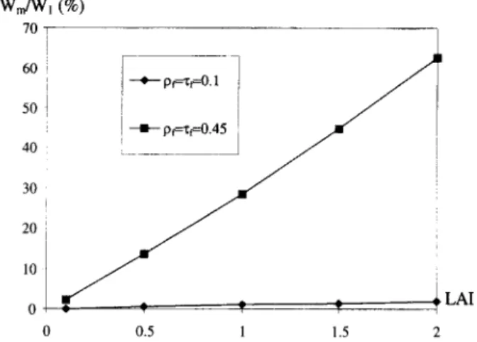
0 i I r I i ! • p~--~--0.45 j 0.5 1 L A I 1.5

Figure 5. Ratio W~,(A/i,Q,~ 0 / W~(A/~,t);-'fl 0 of a leaf

cell as a function of cell LAI. Two cases are considered: toe = 0.9 and rod = 0.2. The LAD is spherical and leaf specular reflectance is neglected.

Figure 5 shows the relative importance of single-scattering Wl(A/~,t),--'f~v) and multiple-scattering W ~ ( A l i , ~ - ' t ) ~ ) source vectors, in the case o f a foliar cellj with a spherical LAD, as a function of the cell LAI. Leaf specular reflec- tance is neglected. Two cases are considered: o9 i = 0.9,

Pd = rd = 0.45, and tot= 0.2, Pd = rd = 0.1. It appears that

W~,(Ali,f~s--'fl~) is all the more important compared to W1(Al, t);-'t)~) than the LAI is large and than the leaf single-scattering albedo is large. For example, with tot--0.9 and LAI = 2, W ~ , ( A / ~ , ~ , ~ ) is equal to 63% of WI(AI~,f~;-'~). This clearly stresses that the multiple- scattering component must not be neglected.

The above-mentioned single and multiple scattering m e c h a n i s m s o c c u r for e a c h i t e r a t i o n of the D A R T model. Some simplifications are introduced for multiple scattering, to reduce computation times; they are shown in the following section.

Hot Spot Effect

The finite size of scatterers within the canopy is respon- sible of the peak in reflected radiation in the retroillumi- nation direction. This is the well known hot spot effect. According to many authors (Qin and Xiang, 1994), this may be a diagnostic tool for canopy structure because its magnitude depends on the size, shape, density, orien- tation, and spatial distribution of foliage elements. For example, in the case of tree canopies its width is often assumed to be governed by the elliptical shape of crowns (Barker Schaaf and Stralher, 1994). In a homogeneous medium, attenuation mechanisms that occur along the scattering direction (f~) are more or tess correlated with those occurring in the incident downward direction (~,), depending on the closeness of directions (t'l,) and (t)~); the correlation value depends on the scattering angle, and on the size sy of the scatterers vs. their depth in the foliar medium. Here, the approach of Kuusk (1985) is adapted in order to take into account the fact

142 Gastellu-Etchegorry et al.

uy(i)" G(i,t2o)- [1 - where

that cells are not infinite horizontal media. It results that the extinction coefficient along direction ( ~ ) of single-scattering source vector [W~(A/~,f~r-'f~)] at a dis- tance Js.<f]o) from the origin point in cell i where reflec- tion took place is not uy(i ) • G(i,f~), but

=

and cos a = f~," t~. 1 2" COS 12

The attenuation of W~(AI~i,f];'*~o ) along the path As~(~) is exp[ - IAs,(a~)a.("~,"~,r)" dr 1.

It must be noted that the hot spot effect is not applied to multiple-scattering source vectors, that is, source vec- tors W~,(A~,~,~f~) in all iterations and source vectors W~(A/~,~r-'~,) in iterations larger than 1.

Iterative Processes with Single and Multiple Scattering

As mentioned above, the DART simulation procedure relies on an iterative method. Two different approaches are adopted for simulating cell interaction mechanisms in the first iteration, that is, mostly single scattering, and in the following iterations.

First Iteration: k = 1, nil. (g2~) = 1, and Q, = 12~u~ The only incident source vector, that is, attenuated direct sun radiation, is a nonfoliar flux (n3~.(~,) -- 1) as- sumed to be nonpolarized (pi.(fl,) -- 0). This sun source vector [Win(0,f~,),Win(0,f],),0] incident on cell i, along the path (A/i, fl~), gives rise to a scattered source vector that escapes cell i along direction (t'2o):

[W~t( Al,,~r-'~), W.f( A l , , f ] , ~ ) , Wp( Al,,~;'*f~o)] with

W.y( Al,.f]r-"t~o) = s~(j,~,,~" WI(A/,,~;'*Oo)

+ °)'~. T( ~T:~°) " s.(j,.~) " W..( Al,,f~, ), w~ w , ( A l , , t ~ , - - , t ~ ) = p~(j,O,,t~o) "

w,(a/,,~,---f~o).

So, we have nf( Al,.fl.,~o) = W~( AI,.O.~O~) + ~ . s~(j.f~) . m~/• W,~(AI.,a.) st(j,~'~s,~"]v) " ~ l d to~

Wso,,( ali, f~,--'f~)

In fact, each cell can be irradiated by different source vectors that propagate along the same direction (f~), W e call • this total number of incident source vectors. The latter are noted W~n(o,~), with o e [1 ~]. Conse-

quently, total scattered radiation that escapes cell i along direction (fly) is

ws~t(Al,(o),a;-.}nv, wnt(a~),w,(a~) with oe[1 ~],

ffi

with

Wq(a~) = ~W.t(Al,(o)n,--.n~ ) o~1 = ~nf(Al,(o),n,,f~).W,~.t(Al,(o),fl.~no), o f f i l Wp(ao) = E Wp( Al,(o),ar-.av) o~1 = Ep(Al,(o),fl,,flo).W~.(Al,(o)fl~f]o). o f f i l

For each interaction (i.e.. Ginteractions) the intercepted radiation W~t(Ali,(o).O~) and the coordinates of the asso- ciated middle point (M~) are stored. Indeed, these only quantities allow one to compute Wx(Ali, O,~O~) and WM(A/.f]r-'fl~). The scalar summation of Wp(Ali(o), f~r-*f]~) vector sources is only possible because all scat- tered source vectors are assumed to have identical polar- ization directions. In the following iteration, cells that have intercepted source vectors in the first iteration become secondary sources.

Further Iterations: k > 1 and I2,e4zr

Incident source vectors [Wi.(O,fl.),W.y.i.(f].),W,.i.(t~.)] stand for already scattered radiation and atmospheric radiation. In a first approximation, considering that inci- dent radiation tends to be isotropic, the polarized scat- tered component is simply assumed to be nil. Thus, with a source vector incident on cell i along the path (A/.O.), the source vector that escapes this cell along direction f~) is

[W~e~t( hl,,O.-'*f]~), W.y( Al,fl.~t~),O]. with

W~at(A/,,t~n--'f~) -- W~(A/,,f]~--'~) + WM(Al,t~.'-'f]o), Wq( Al,,O.--'O~) = nJ~.(f~.) " ls~(j,~.,fl~ ) " W~(Al,,fl.~fl~)

T( as',t~O) . sMO, flo) .

°~w,~,(a/,,fl,)].

In fact, each cell is irradiated by a number ~ of source vectors 2]/i.(f~.i(o)) that propagate along different inci- dent directions f~.(o) in the 4re space, with oe [1 ~ ] and ne [1 JF]. C o n s e q u e n t l y , total s c a t t e r e d r a d i a t i o n [W~¢~t(C,~v)] that escapes cell i along direction (f~o) is

Radiative Transfer of Heterogeneous Vegetation Canopies

143

Use of the approach of iteration 1 would lead to store all middle points M~(o), the intercepted radiation W~,t (Ali,O,(o)), and the associated incident directions (f~(o)), with o611 ~]. This would demand a huge computer memory capacity with large scenes. Thus, another ap- p r o a c h is a d o p t e d . W h e n an i n c i d e n t radiation [W(0,t)~)], with n~ [1 ~//~, is intercepted, resulting scat- tered specific intensities I(A/.f~--'f~) and I.f(A/~,~--" t)~), associated with source vectors W(A/i,~n~t~) and W.f(Al.t).~£)v), are computed for all N(D.v) directions, and their distribution is represented by a spherical expansion:

/=L mffil

l(Al,,~,--'f~v) = Z ~,,

Clm(i,k)'YIm(O, tp),

l=Om=-I

where Ylm(O,~) are the normalized spherical harmonics and Clm the associated coefficients. L is an integer num- ber that indicates the order of the expansion. It can be selected by the operator. In real form the normalized spherical harmonics are defined by

Nlm'elm(COS 0)" cos(m(~) ifm > 0, Yl,~(O,~) = N~'P~o(COS 0) / ~/~ ifm = 0,

NIm'Pl~(COS 0)'sin(Italy) i f m < 0, where the elm(x) factors are the associated Legendre polynomials and the normalizing constants Ntm are given by

Nl 12/+ 1 . (1 -[ml)!

m--- 5~ 27[7

(1

+ Iml)!

The Clm(i,k) coefficients related to the kth scattering order in cell i are derived from

~2~fn

C,m(i,k,O,)= J0 Jo l(Al''O~of~)'Y'(O#)'sin O'do'dO

= ~ Wscat(~')s'-~av)'Ylm(Ov).

v=t

The coefficients Clm(i,k,t),) are actually computed during the ( k - 1)th iteration order, both for the total W~at(f~) and the nonfoliar W,f(f~) radiation components. After each interaction with cell i, the n e w

Clm

coefficients are added to the Cl~ coefficients associated with radiation previously scattered in that cell:

Cl,~(i,k) = ~Ct~(i,k,f~,), w h e r e ~ i s the total number o ~ l of radiation incident on cell i.

The scattered source vector [W~cat(i,~v), Wnf.~cat(i,f~v), 0] that exits cell i is computed in the kth iteration:

lffiL mfl

Wscat(i,~)v) = ~ ~,,

Ctm(i,k)"

Ytm(f~)" A ~ ,

/ftOm= -l

lffiL m=l

C,m.nf(i,k)"

At o.

l=Om= -l

The spherical harmonics formulation may not be well adapted if the transfer matrix is very anisotropic. Such an anisotropy occurs with opaque media such as soils. For example, an horizontal opaque surface displays a discontinuity of the scattered flux for directions within the plane of the interface. Moreover, it may comprise a strong specular component, for example, due to direct sun illumination. In the presence of such surfaces the following approach must be adopted: Before computing the Ctm coefficients, the transfer matrix is extended to the forward hemisphere. Thus, in the special case of an horizontal surface, we use the relation

I(i,rt - 0,~) = I(i,O#).

This approach is interesting because it smoothes the integrated term I(i,O#), which results in a more accurate approximation with a fixed number of Ctm coefficients. This extension is especially designed for soil and water cells.

The spherical harmonics expansion is well adapted to approximate relatively smooth functions defined on the sphere, with a finite number of terms. This number is much less important than the total number N of discrete directions. A diffuse smoothly varying distribu- tion of specific intensity will typically require fewer coefficients than a very directional one. Moreover, the spherical harmonics expansion is well adapted to the incremental computation of scattered radiation resulting from successive impinging interaction mechanisms, for each cell. After a scattering event occurs in cell i, we have the following sequence of operations: computation of the angular distribution of the scattered source vector W(i,f~) and W~f(i,f~v), computation of the associated Clm and Ctm.,y coefficients, and adding these coefficients to the already accumulated Cry(i) and Clm,,f(i) coefficients. The spherical harmonics expansion is not used dur- ing iteration 1. Indeed, the simple knowledge of the intercepted radiation and of the associated middle point, combined with the fact that sun direction is known, is less computer memory demanding than the spherical harmonics-based approach. Moreover, and above all, it leads to more accurate results because scattered radia- tion that results from monodirectional incident radiation may be highly anisotropic, which is poorly represented by a spherical harmonics expansion with a limited num- ber of terms.

Interaction Mechanisms of Nonleaf Cells

Interaction mechanisms associated with non leaf cells are briefly introduced below.

Soil Cells

Their optical properties are represented by scattering transfer matrices Tso~(~s,~) derived from measurements

144 Gastellu-Etchegorry et al.

or computations with whatever available soil bidirec- tional reflectance model• Associated polarization trans- fer matrices are noted T~.soa(~,~). Only surface interac- tions are simulated. The geometrical path of a soil scattered radiation within the scene is simulated from the center of the irradiated soil cell face. In order to take into account topography, soil cell interactions are handled separately for each cell face. So, during the direct sun illumination phase, the energy intercepted is stored for each individual face of soft cells. In the following iteration each face gives rise to secondary source vectors, with a priori defined scattering direc-

tions, for example, an upper horizontal face scatters upwards only• Similarly, during subsequent iterations, radiation interactions occur also on individual faces, and Ctm coefficients are computed and stored for each illuminated face of soil cells.

In a first approximation, polarization is simulated, independently of the polarization degree of the incident radiation. Naturally, any radiation scattered by a soil cell of type j has the same non foliar factor nf.(f~) as

the incident radiation [W~n(O,~,)]. Thus, the resulting scattered source vector along direction (~v) is

[ Wseat( ~v), Wnf, scat( ~'~v), Wp,scat( ~'~v) ],

with

w, t(f o) =

= • W,c ,(oo) a n d

Wp.scat(~v) = Tp,~o,,(j,~,,~)" Wi,(O,~).

The expression of source vectors scattered by a soil cell depend on the iteration order:

Iteration k = 1:

0=1

= T,o,,(j.t~.,f~)" Z W~.(O,a,(o)), 0=1

Wnf, scat(~'~v) -~ Z Wnf.scat(~s(O) ''}~'~v) "~

Wscat(~'~v) ,

0=1 Wp,~,t(t~v) = pt(j,~,,f~)'Wsc,t(f~v) with T.,,o,,(j,f~..f~o) = T~oil(j,O,,fl~) Iteration k > 1: g~ d = 0. Trunk Cells

Trunk cells are undoubtedly of minor importance in many cases. Trunk cells are characterized by scattering

Ttrunk(~r~n'-~'~"~v)

and polarization

Tp,trunk(~'~n'~'~d

transfer matrices. Polarization mechanisms are modeled without taking into account the polarization of the incident radiation Wi,(0,f~8). For example, each trunk cell can be characterized by an hemispheric reflectance coefficient /Ttrunk and an extinction parameter t/. The latter is inde- pendent of the incident radiation (~) and equal to the ratio of the vertical trunk surface by the surface of the associated vertical cell face. In fact, several trunk cells may be crossed when a source vector W(~,) encounters a trunk. Let qmax be the maximum value of the r/terms associated with the cells that are crossed• Then, the transmission coefficient of the incident source vector W(f],) is

T(O) = 1 - nmax.

Thus, T(~) ~ 1 if ~max " ~ 0 (i.e., empty cell) and t/~,~

i if T ( ~ ) -~ 0 (i.e., 100% trunk cell).

So, in a first approximation the trunk scattering transfer matrix Tt~mk(~,"~) can be simply defined by

n

where ~c is the direction normal to the irradiated cell

faces•

Radiation interaction with trunk cells are processed on a face per face basis, in the same way as soil cells• The six faces can become secondary scatterers. In fact, source vectors are scattered only by cell faces that are directly irradiated by the incident radiation. Naturally, a source vector scattered by a trunk cell has the same non foliar component nf(f~) as incident radiation• Thus,

a number @of incident source vectors [Win(0,f],¢o))] leads to

[o~lWseat(~'~n(o)"'}~'~v),Wnf, scat(~']v,

Wp, scat(~'~v)].

Iteration k = 1:

tY

Z w,

0=1

Wp, seat(~'~v) = Z

PlO, fls,~'~v) •

W~.t( al,(o),f]."}t~)

o=1 ---- px(j, Os,~'~v)" Wscat(Ov). Iteration k > 1:

o=1

w,•soa,(ao) = 0. Water Cells

Similarly to soil surfaces, water surfaces are modeled as a unique layer of water cells, and their upward reflectance characteristics are represented by scattering transfer functions Tw,ter(~,~v) and polarized transfer functions