Studies on Management of Emergency Service Systems

(1)

Studies on Management of Emergency Service Systems

AKBAR KARIMI

Département de mathématiques et de génie industriel

Thèse présentée en vue de l’obtention du diplôme de Philosophiæ Doctor Mathématiques

Août 2019

c

(2)

Cette thèse intitulée :

Studies on Management of Emergency Service Systems

présentée par Akbar KARIMI

en vue de l’obtention du diplôme de Philosophiæ Doctor a été dûment acceptée par le jury d’examen constitué de :

Antoine SAUCIER, président

Michel GENDREAU, membre et directeur de recherche Vedat VERTER, membre et codirecteur de recherche Fabian BASTIN, membre

(3)

DEDICATION

(4)

ACKNOWLEDGEMENTS

First and foremost, I thank Michel Gendreau and Vedat Verter for giving me this opportunity and for the extended financial support over the years. They both have been extremely and undeservedly nice and accommodating to me, for which I feel equal parts fortunate and grateful.

The financial support for the research conducted by the author, which is partly reported in this thesis, has been jointly provided, with no specific order, by the Interuniversity Centre on Enterprise Networks, Logistics and Transportation (CIRRELT), the Department of Industrial Engineering and Applied Mathematics of the Polytechnique Montréal, and the CREATE Program on Healthcare Operations and Information Management. Their support is greatly appreciated.

I am grateful to the kind, friendly and supportive staff at CIRRELT, the Polytechnique Montréal, the department of Orthopedic Surgery at the Jewish General Hospital, and other medical care centers I have visited in the last few years; in particular, I wish to extend my special thanks to Lucie L’Heureux, Lucie-Nathalie Cournoyer, Guillaume Michaud, Delphine Périé-Curnier, Melisa Regalado, Suzanne Guindon, Diane Bernier, Amal Bennani, Dr. Peter Jarzem, Martine Dahan, Jason Skolar, and Émillie Fournier.

My transition to life abroad was greatly eased by the company of my little circle of good friends with whom I share memories I will cherish forever.

I wholeheartedly thank Mont Royal Park and Saint Joseph Oratory for being places where, if you go at the right time, polarities meet, singularities form and the whole physicality thing takes the back seat, at least for a few fleeting moments.

Last, but not least, I send my love to my parents, for doing what parents do best, and for going the extra mile of creating two cute siblings for me, so I wouldn’t need to go out of the house to find kids, of either gender, to fight with—sometimes, to the point of inducing near death out-of-body experiences—and later on, rely on as unbounded sources of trust and compassion, when trust and compassion are as hard to come by as practical applications for the ideas presented in this manuscript.

(5)

RÉSUMÉ

Forts des outils de la théorie des files d’attente, de la géométrie stochastique et des exten-sions développées en cours de route, nous présentons des modèles descriptifs de systèmes de services d’urgence organisés en fonction du potentiel de limitation explicite des distances de dispatching avec une fidélité accrue du modèle et une stratégie de dispatching pour atteindre des performances maximales avec des ressources limitées. En utilisant le terme «sauvegardes partielles» pour faire référence à des règles d’expédition avec des limites explicites sur les distances d’expédition, nous étendons d’abord le modèle classique de mise en file d’attente hypercube pour inclure des sauvegardes partielles avec des priorités. La procédure éten-due pourra représenter les systèmes de services d’urgence dans lesquels le sous-ensemble de serveurs pouvant être envoyés à une demande d’intervention d’urgence dépend de l’origine et du niveau de service demandé. Cela permet de développer des modèles d’optimisation dans lesquels le concepteur du système laisse le choix des unités de réponse pouvant être envoyées dans chaque zone de demande et peut être intégré à l’espace de la solution avec d’autres variables de décision d’emplacement ou d’allocation. La nouvelle méthode descriptive et les modèles d’optimisation sur lesquels reposent les plans de répartition et de répartition opti-maux correspondants devraient indiscutablement améliorer les performances et mieux refléter le comportement réel des répartiteurs lorsque la configuration instantanée du système con-stitue un facteur majeur dans la prise de décision. Par la suite, nous étendons notre analyse. des déploiements statiques couverts par le premier modèle vers des systèmes à relocalisation dynamique. En faisant des hypothèses d’uniformité sur les origines des demandes de service et les emplacements des unités d’intervention, nous développons un cadre théorique pour une évaluation rapide et aléatoire de la performance du système avec une politique de sauvegarde partielle donnée et des résultats donnés spécifiés en fonction du temps de réponse. Le modèle général permet de révéler tout potentiel théorique d’amélioration des performances du sys-tème en utilisant des stratégies de dispatching de secours partielles aux stratégies tactiques ou opérationnelles, sans connaître les détails de la méthode de relocalisation dynamique utilisée ni même de la distribution de la demande au-delà du taux total d’arrivée et de la densité. Nous présentons des résultats auxiliaires et des outils à l’appui de notre traitement des systèmes de service d’urgence avec sauvegardes partielles, notamment des notes sur les distributions de distance avec des effets liés et quelques lois de conservation du débit liées aux situations de file d’attente rencontrées dans le cadre de ce travail.

(6)

ABSTRACT

Armed with tools in queuing theory, stochastic geometry, and extensions developed along the way, we present descriptive models of emergency service systems organized around and emphasizing the potential of explicitly limiting dispatch distances in increasing model fidelity and as a dispatching strategy to achieve maximal performance with limited resources. Borrowing the term ”partial backups” to refer to dispatch policies with explicit limits on the dispatch distances, we first extend the classic hypercube queuing model to incorporate partial backups with priorities. The extended procedure will be able to represent emergency service systems where the subset of servers that can be dispatched to a request for emergency intervention depend on the origin and level of service requested. This allows for development of optimization models where the choice of response units eligible for dispatch to each de-mand zone is left to the system designer and can be integrated into the solution space along with other location or allocation decision variables. The new descriptive method and thus the optimization models built upon and the corresponding optimal location and dispatch plans, should arguably lead to better performance and better reflect the actual dispatchers’ behavior where the instantaneous system configuration constitutes a major factor in making assignment decisions.

We next extend our analysis of static deployments covered by the first model to systems with dynamic relocation. Making uniformity assumptions on the origins of service requests and locations of the response units, we develop a theoretical framework for quick and dirty evaluation of the system performance with a given partial backup policy and a given outcome specified as a function of response time. The general model, makes it possible to reveal any theoretical potential to improve system performance by employing partial backup dispatching strategies at tactical or operational, without knowing the details of the dynamic relocation method used or even the demand distribution beyond the total arrival rate and the density per area.

Finally, auxiliary results and tools supporting our treatment of emergency service systems with partial backups are presented, which include notes on distance distributions with bound-ary effects and a few rate conservation laws related to the queuing situations we encountered in this work.

(7)

TABLE OF CONTENTS

DEDICATION . . . iii

ACKNOWLEDGEMENTS . . . iv

RÉSUMÉ . . . v

ABSTRACT . . . vi

TABLE OF CONTENTS . . . vii

LIST OF TABLES . . . x

LIST OF FIGURES . . . xii

LIST OF SYMBOLS AND ACRONYMS . . . xiv

LIST OF APPENDICES . . . xv

CHAPTER 1 INTRODUCTION . . . 1

1.1 Basic concepts and definitions . . . 5

1.1.1 Queuing theory . . . 5

1.1.2 Spatially distributed service systems . . . 9

1.1.3 Discrete event simulation . . . 12

1.1.4 Analytical versus simulation models . . . 15

1.2 Research objectives . . . 17

1.3 Plan of the thesis . . . 18

CHAPTER 2 LITERATURE REVIEW . . . 19

CHAPTER 3 SYNTHESIS OF THE WORK AS A WHOLE . . . 21

CHAPTER 4 ARTICLE 1: PERFORMANCE APPROXIMATION OF EMERGENCY SERVICE SYSTEMS WITH PRIORITIES AND PARTIAL BACKUPS . . . 23

4.1 Introduction . . . 23

4.2 Literature Review . . . 25

4.3 Formulation . . . 28

(8)

4.3.2 Immediate Dispatches . . . 31

4.3.3 Delayed dispatches . . . 36

4.4 Algorithm . . . 39

4.5 Numerical Experiments . . . 42

4.5.1 Validity of the Full-backup Assumption . . . 46

4.5.2 Accuracy of the Approximation . . . 47

4.5.3 Complementary Computational Results . . . 48

4.6 Conclusions . . . 49

4.7 Complementary Computational Experiments . . . 50

CHAPTER 5 DISTANCE DISTRIBUTIONS WITH BOUNDARY EFFECTS . . . 53

5.1 Euclidean Metric . . . 54

5.2 Manhattan Metric . . . 58

5.2.1 Remarks . . . 62

CHAPTER 6 ON OPTIMAL DISPATCH POLICIES FOR EMERGENCY SERVICE SYSTEMS WITH DYNAMIC RELOCATION: A QUEUING THEORETICAL FRAME-WORK WITH APPLICATIONS . . . 65

6.1 Mathematical Model . . . 69

6.1.1 Distribution of the number of busy servers . . . 69

6.1.2 Probability of Loss and Queue . . . 70

6.1.3 Queuing Delay . . . 72 6.1.4 Dispatch Distance . . . 78 6.1.5 Response Time . . . 90 6.1.6 Response Outcome . . . 93 6.1.7 Service Time . . . 94 6.1.8 The Algorithm . . . 95

6.2 Drone-Van Combo Systems . . . 95

6.3 Examples . . . 98

6.3.1 Drones to deliver AEDs to cardiac arrest incidents in an urban envi-ronment . . . 99

6.3.2 Queuing ESS . . . 106

6.4 Remarks . . . 108

CHAPTER 7 CONDITIONAL EXTENSION TO LITTLE’S LAW . . . 121

7.1 Results . . . 121

(9)

CHAPTER 8 GENERAL DISCUSSIONS . . . 131

CHAPTER 9 CONCLUSION AND RECOMMENDATIONS . . . 133

9.1 Summary of the Work . . . 133

9.2 Limitations . . . 133 9.3 Future Research . . . 133 REFERENCES . . . 135 APPENDICES . . . 141 A.1 Theorem 1 . . . 141 A.2 Theorem 2 . . . 144

A.3 Correction of State Probability Approximations . . . 144

B.1 Sensitivity to Service Time Distribution . . . 148

B.2 Impact of Location and Priority Dependent Service Times . . . 150

B.3 Impact of System Workload . . . 152

B.4 Computational Expense Reduction . . . 153

C.1 Loss Drone System . . . 158

(10)

LIST OF TABLES

Table 4.1 Comparison of server workloads estimated by the model and simulation. 42 Table 4.2 Comparison of immediate dispatch rates estimated by the model and

simulation (in parentheses). . . 42

Table 4.3 Comparison of delayed dispatch rates estimated by the model and sim-ulation (in parentheses). . . 42

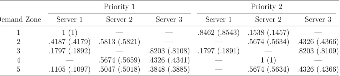
Table 4.4 Comparison of average waiting times (in minutes) and fractions of calls queued estimated by the model and simulation (in parentheses) for the system with queues. . . 43

Table 4.5 Components of the service time (in minutes). . . 44

Table 4.6 Values of the travel time model parameters. . . 44

Table 4.7 Coverage threshold scenarios considered in the experiments. In each scenario, the maximum coverage threshold for each priority level is given in kilometers. . . 45

Table 4.8 Estimation errors assuming full-backups*. . . 47

Table 4.9 Estimation errors for the loss system (in %) . . . 48

Table 4.10 Estimation errors for the queuing system (in %) . . . 48

Table 4.11 Waiting time estimation errors with actual values from simulation in parentheses (in minutes) . . . 48

Table 6.1 Parameters used in the first example . . . 100

Table 6.2 Parameters used in the second example . . . 107

Table B.1 Service time distribution scenarios used in the experiments. . . 150

Table B.2 Server workload estimation errors for different simulated service time distributions (in %). . . 151

Table B.3 Total dispatch rate estimation errors for different simulated service time distributions (in %). . . 152

Table B.4 Waiting time estimation errors for different simulated service time dis-tributions (in minutes). . . 153

Table B.5 Server workload estimation errors with alternative scenarios of service time dependence on priority and location (in %). . . 153

Table B.6 Total dispatch rate estimation errors with different scenarios of service time dependence on priority and location (in %). . . 154

(11)

Table B.8 Immediate dispatch rate estimation errors for different load factors (in %). . . 155 Table B.9 Delayed dispatch rate estimation errors for different load factors (in %). 155 Table B.10 Waiting time estimation errors for different load factors, with the actual

simulation values in parentheses (in minutes). . . 156 Table B.11 Average server workloads for different load factors. . . 156

(12)

LIST OF FIGURES

Figure 1.1 Service time components . . . 11 Figure 1.2 General flowchart of discrete event simulation . . . 14 Figure 4.1 Comparison of errors in approximating the state probabilities of a

pri-ority partial service queue by the corresponding non-pripri-ority version (M/M/[N]) and an M/M/N queue. Reported are the mean absolute errors for a system with three priority levels and different numbers of servers. . . 32 Figure 4.2 Distribution of the number of busy servers and the Z correction factors

for an example queuing system with N = 10, µ = 1.4 and different arrival rate scenarios given by: A) [λc] = [0, 0, 0, 0, 0, 0, 0, 0, 0, 10], B) [λc] = [10, 0, 0, 0, 0, 0, 0, 0, 0, 0], C) [λc] = [1, 1, 1, 1, 1, 1, 1, 1, 1, 1], D) [λc] = [2, 2, 2, 2, 2, 0, 0, 0, 0, 0], and E) [λc] = [0, 0, 0, 0, 0, 2, 2, 2, 2, 2]. . . 51 Figure 4.3 Illustrative Example . . . 52 Figure 4.4 Demand distribution and hospital locations. . . 52 Figure 5.1 Distribution of the Euclidean distance to the n-th nearest neighbor out

of N u.i.d random points. . . . 63 Figure 5.2 Distribution of the Manhattan distance to the n-th nearest neighbor

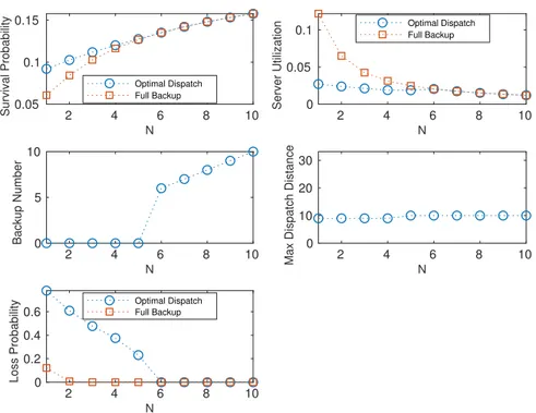
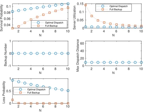
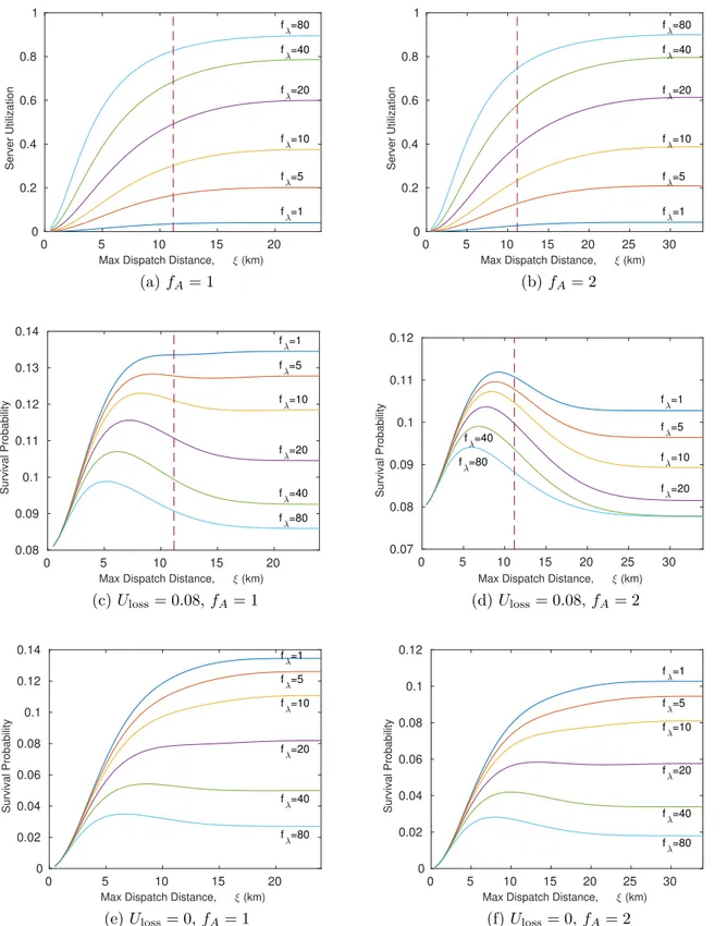
out of N u.i.d random points. . . . 64 Figure 6.1 Response outcome functions used in the example applications . . . . 101 Figure 6.2 Analysis of the optimal dispatch policy for the drone system and fA= 1102 Figure 6.3 Analysis of the optimal dispatch policy for the drone system and fA= 2103 Figure 6.4 Analysis of the optimal dispatch policy for the drone system and fA= 4104 Figure 6.5 Analysis of the optimal dispatch policy for the drone system and fA= 8105 Figure 6.6 Performance of the zero-backup drone system with different loads . . 111 Figure 6.7 Performance improvement using zero-backup dispatch policy in the

drone system with three servers . . . 112 Figure 6.8 Server utilization and survival probability for the zero-backup drone

system with different fleet sizes and service areas . . . 113 Figure 6.9 Performance improvement using zero-backup dispatch policy in the

drone system with baseline demand (fλ = 1) and Uloss= 0.08 . . . . . 114

Figure 6.10 Analysis of the optimal dispatch policy for the queuing EMS and fA= 1114 Figure 6.11 Analysis of the optimal dispatch policy for the queuing EMS and fA= 2115 Figure 6.12 Analysis of the optimal dispatch policy for the queuing EMS and fA= 4115

(13)

Figure 6.13 Analysis of the optimal dispatch policy for the queuing EMS and fA= 8116

Figure 6.14 Service quality for the zero-backup queuing EMS . . . 117

Figure 6.15 Performance improvement using zero-backup dispatch policy in the queuing EMS with three servers . . . 118

Figure 6.16 Server utilization and service quality for the zero-backup queuing ems with different fleet sizes and service areas . . . 119

Figure 6.17 Performance improvement using zero-backup dispatch policy in the queuing EMS with baseline demand . . . 120

Figure 7.1 The ordered arrivals and departures . . . 125

Figure A.1 The birth-death model to compute state probabilities . . . 145

Figure A.2 Comparison of the state probability estimation errors with and without the correction scheme averaged over randomly generated cases with 20 servers (N = 20) and varying workloads. The estimation error is computed as PN n=1|Pnmod− Pnsim|. . . 147

Figure B.1 Variation of estimation errors and computation times with the update frequency. . . 157

Figure C.1 Simulation versus model: loss system, N = 2, fλ = 1, fA= 1. . . 159

Figure C.10 Simulation versus model: queuing system, N = 4, fλ = 1, fA= 1. . . 168

(14)

LIST OF SYMBOLS AND ACRONYMS

ESS Emergency Service System EMS Emergency Medical Services FCFS First Come, First Served LCFS Last Come, First Served ASTA Arrivals See Time Averages

PASTA Poisson Arrivals See Time Averages PPP Poisson Point Process

u.i.d Uniformly and Independently Distributed i.i.d Identically and Independently Distributed

(15)

LIST OF APPENDICES

Appendix A Proof of Theorems in Chapter 4 . . . 141 Appendix B Complementary Computational Experiments for Chapter 4 . . . 148 Appendix C Comparison of Simulation and Approximation Models for ESS with

(16)

CHAPTER 1 INTRODUCTION

The primary goal of an Emergency Service System (ESS), quite obviously, is to provide emer-gency care to customers in immediate need for it. The ability of the system to provide such services is thus a natural measure of performance. To achieve adequate performance, the system needs to be well designed and adequately resourced. The optimal performance, how-ever, cannot be achieved without reliable tools to assess the suitability of a given tentative design candidate. Simulation models remain the gold standard to assess complex systems and allow the designer to evaluate design and operation scenarios with great flexibility in terms of the desired level of detail and accuracy. The downside to simulation, however, is the computational expense of scenario analysis which in some applications can be quite prohibitive. For example, consider a dynamically relocating emergency service system in which the dispatchers will send the available response units to new waiting stations every time time the number of free vehicles changes. In many cases, such relocation decisions are based on a real-time evaluation of different and potentially many candidate relocation plans of which the best ones are selected. The time needed for evaluation of these candidate plans can arguably become prohibitively long if a simulation model is used, unless it is carried out on an unusually capable computing platform. In these cases, mathematical models with their faster computation times come to our aid allowing a wider system optimization appli-cations such as real-time dynamic relocation planning and, in general, less computationally demanding analyses that can be performed on less powerful computing systems or in shorter times. The popularity and range of various descriptive mathematical models incorporated into prescriptive optimization models proposed in the literature attests to the effectiveness of such tools in helping the system analysts in making better management decisions at tactical, operational, and strategic levels. If desired, detailed simulation models can be employed in further evaluation of an initial set of decisions obtained using these primary optimization models. We will briefly compare simulation and analytical approaches and their respective straights at the end of this chapter.

Regardless of the objectives and constraints of an optimization model, the quality of the solutions obtained directly depends on the validity of the underlying descriptive model used in representing the system at hand as closely as possible. Therefore, it will always pay off to further improve a given descriptive model so that it better reflects the realities of the system or operation we seek to optimize or analyze. The hypercube queuing model of Larson (1974) and its approximate form developed by, again, Larson (1975), is the classic method of modelling a spatially distributed queuing system, and in particular, an ESS. This

(17)

model, and its numerous extensions, have been widely used by researchers and practitioners alike in development of optimization models of various emergency service operations. The original version of the method relies on several restricting and unrealistic assumptions that can limit the range of situations in which the model can reasonably act as a proxy to the system considered. Over the years, several attempts have been made to relax some of these assumptions; however, the assumption that the closest free response vehicle will always be sent to an incoming request for service regardless of the origin of the call, and in particular, its distance from the dispatched vehicle, remains to this day. This is basically the assumption of full backups as opposed to a policy of partial backups in which each response vehicle is responsible only for providing service to an arbitrary subset of demand zones or service region. The assumption of full backups in most practical applications will be in disagreement with how the actual system is operated. In some cases, this might be due to the strict zoning or allocation strategies in place; for example, a fleet of police patrol cars where each patrol car is responsible for a well-defined sector of the service region. A full backup assumption is clearly not valid for this case. Physical limitations of the response units may as well impose a limit on the maximum travel distance, rendering the full backup assumption inaccurate. For instance, an ESS operation comprised of aerial drones will be best modelled as a partial backup system since the maximum flight range of virtually all drones available today is limited by the capacity of the batteries powering them. Finally, the full backup assumption may fail to reflect dispatchers’ behavior in assigning response vehicles to incoming calls. To see this clearly, suppose a request for service is received where the closest vehicle is busy and the second closest response unit is free but is located much farther from the call origin. Now, if the dispatcher estimates the close-by vehicle to finish its current job in less time than it would take the second vehicle to arrive at the scene, then he or she will most probably wait for that busy vehicle to become free and then get immediately dispatched to the new call. Under the assumption of full backups, however, the farther vehicle will be selected for dispatch regardless of the unreasonably long travel distance and response time it results in. The assumption of full backups in this situation will of course be less realistic and valid when the outcome of the intervention is more strongly impacted by the response time. Responding to highly urgent requests such as incidents of Out-of-Hospital-Cardiac Arrests (OHCA) presents a prime example of a highly time-critical operation for which dispatching a vehicle over distances over a certain limit will result in very low probability of patients surviving. These observations establish the importance of relaxing the full backup assumption in analysis of emergency service systems and motivate us to develop new descriptive models or modify the existing methods in which the more realistic partial backup policy is explicitly incorporated into the model. The notion of partial backups is thus the main theme of the present work

(18)

and forms the basis of the models we develop in subsequent chapters.

To provide a more comprehensive treatment of emergency service systems, we consider both static and dynamically relocating deployments and try to develop models for performance ap-proximation of the system with these respective deployment mechanisms. In a static deploy-ment, the response units are assigned fixed waiting stations from which they are dispatched to locations of emergency incidents and travel back to when the service is completed. In an ideal static deployment, the response units are arranged such that the best possible coverage is provided to the entire service region. The notion of adequate or good coverage, however, can be interpreted in many ways and encompass different and often competing objectives. For instance, with the maximum coverage or outcome as the main objective, deployments in which response units are placed closer to areas with higher demand concentrations will typically yield the best results. On the other hand, if a measure of equity in service pro-vision is instead selected as the performance objective, then the optimal deployments will normally have the response units more uniformly distributed over the service region to guar-antee sufficiently reliable access to services independent of location. In a deployment with periodic relocation, the planning horizon is divided in several time periods each with their own set of optimal locations for the waiting stations. Each of these static deployments is optimized for the corresponding demand configuration observed or predicted for that period. The number of vehicles deployed in each period may also be different. The system then se-quentially switches through these set of static deployments in an attempt to adapt to varying operating conditions over the planning horizon. The geographic distribution of demand or traffic conditions are examples of operating conditions that change with time and can be effectively addressed through periodic deployments. Periodic deployment plans can be easily constructed by repetitive applications of the static deployment models and thus, for the most part, do not need special mathematical devices beyond what is needed to account for the costs and constraints associated with transitions between the periods.

A deployment with dynamic relocation tries to maintain an adequate coverage of the service area by relocating the free response units to new positions whenever the number of available vehicles changes; that is, each time a vehicle finishes its current job and becomes available thus increasing the number of free units, or when a vehicle gets dispatched to a new incoming call thus decreasing the number of free units. Unlike the periodic redeployment which reacts to the changes in the underlying operating conditions, the goal of dynamic relocation is to continuously maintain adequate coverage of the service area with an ever-changing number of available server at any given moment. These systems can also be treated with static deployment models by first obtaining a pre-calculated set or sets of optimal static deployments for fleets of size n = 1, 2, · · · , N with N the actual number of deployable response units, and

(19)

then relocating the vehicles in real-time according to the optimal static deployment with n units whenever the number of free vehicles drops or increases to n. This set of pre-determined deployments is commonly known as a compliance table which is basically a look-up table of acceptable arrangements of response units for every number of available vehicles. Whenever a relocation is required, the dispatcher will re-position the currently available vehicles to new waiting stations according to a relocation plan he or she deems most appropriate for the situation among the candidates given in the compliance table. This approach does not require any real-time computation as the compliance tables are obtained offline.

A dynamic relocation deployment, however, can also be implemented in a more sophisticated fashion in which relocation decisions are computed in real-time whenever the number of available units changes. This approach has the clear advantage of taking into account the exact instantaneous state of the system in calculating new waiting spots for each of the free vehicles. This is important since other factors besides maintaining adequate coverage should be taken into consideration while making relocation decisions. Most notably, a good relocation decision should preferably minimize both the number of vehicles that should be relocated and also the corresponding travel distances. Compared to compliance tables, real-time computation of the new waiting spots provides a greater flexibility for incorporating all these contributing aspects in generating best relocation decisions. Although the real-time calculation of the optimal locations requires considerably higher computational power compared to the compliance table method, the actual problems to be solved can still be considered as instances of static deployments with appropriate constraints and objectives reflecting what the manager considers acceptable and desired in a good relocation plan. As we see, the ability to solve static deployment problems is all we need for analysis and design of static, periodic, compliance table and real-time dynamic deployments. This highlights the importance and value of developing more accurate mathematical methods such as the hypercube queuing model for evaluation of static deployment scenarios. As stated earlier, the quality of the location and relocation plans and compliance tables obtained will be directly dependent on the quality of the underlying mathematical model used to describe the steady-state behavior of the system for a given static deployment. In the first main contribution of the thesis, presented in Chapter 4, we take a step towards this very objective of increasing the accuracy and applicability of the approximate hypercube queuing model by relaxing the assumption of full backups and allowing for partial backups with priorities. As we will see, the original version of the approximate hypercube queuing model will lead to large approximation errors when used to estimate the steady-state behavior of a system with partial backups. The proposed extension of the hypercube model, however, performs well in predicting the equilibrium behavior of the system with priorities and partial backups. This opens a door to

(20)

new optimization models in which we augment instances of system deployments by specifying the subset of demand zones covered by each response unit in addition to the location in which each unit is deployed. This more refined view of the system combining the location and allocation decisions, allows for a more realistic and detailed description of the actual deployment scenarios encountered in practice. Armed with the extended hypercube model with partial backups, one can now predict the steady-state behavior of the system for a given set of tentative location and allocation decisions. Evaluation of many such sets of combined decisions within an optimization loop with appropriate objectives and constraints will then give us an optimal location and allocation decisions we need for a static deployment.

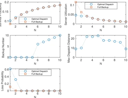
While the extended hypercube model developed in Chapter 4 aims at accurate prediction of the performance of system deployments with partial backups, the mathematical model pre-sented in Chapter 6 tries to quantify the impact of partial backup policies on the performance of systems with real-time dynamic relocation. Making simplifying assumptions, including the uniformity of the distribution of call locations and of the response units, we build an abstract model that can be used to obtain the expected performance of the system operating under a given partial backup dispatch policy. The partial backup policy in this case is defined as the maximum number of neighboring response units considered for dispatch alongside a limit on the maximum dispatch distance for the rest of the units. Finally, Chapters 5 and 7 contain some supporting results used in development of the main models described above.

1.1 Basic concepts and definitions

In this section, we briefly go over some basic concepts related to the topics discussed in this thesis. These introductory sections are mainly aimed at a reader not familiar with the basics of queuing theory and related topics. We also clarify the terminology used in the text. We first give a basic overview of queuing theory including an introduction to Kendall’s notation for queuing systems followed by an introduction of spatially distributed service systems and the tools we have for studying these systems. We then highlight the value and applications of analytical and simulation models in studying service systems. Finally, we provide a concise statement of the purpose and objective of the dissertation together with a plan of the thesis.

1.1.1 Queuing theory

The main contributions of this thesis rely heavily on queuing theory, a discipline within the mathematical theory of probability, devoted to the study and prediction of waiting lines and waiting times. Queuing theory results are most often used in operations research to aid in

(21)

making decisions about the resources required to provide a service with a certain level of quality. Besides operations research and industrial engineering, queuing theory ideas have been widely applied in telecommunication, traffic engineering, computing, forestry and many more design and management problems.

A queuing station or node (or simply a queue) can be viewed as a black box representing a service station where customers arrive, stay for a while to receive service, and depart once the service is completed. A supermarket checkout line is a cliched example of a queuing node (or system). Customers arrive, possibly wait in a line for their turn, eventually get processed by the cashier and then leave.

Usually, we have some information regarding the inside of a queuing model; at the very least, the number of servers, that is, for example, the number of cashiers in the supermarket line, should be specified. In a multi-server queue, that is a queue with more than one servers, any server can process an arriving customer and can start working on a new arriving or waiting customer after the current service is completed. This is the most usual situation and can be used, for example, to represent a single waiting line in a bank processed by multiple tellers. In other multi-server models, however, we might have different customer and server types with policies specifying the types of customers that can be processed by each server type. Call centers are a good example of this kind of queuing systems where agents are trained in one or more specific areas and thus can only accept callers who request a certain type or types of services. This is generally known as a skill-based routing as customers are assigned to suitable servers based on their matching skills. In a multilingual call center, for example, a skill-based routing may be used based on the languages spoken by the agents and the customers. Queues with skill-based routing are remarkably difficult to analyze with limited relevant theoretical results published in the literature. We note that the queuing system with partial service introduced in Chapter 4 and revisited in Chapter 6, can be considered queuing models with skill-based routing. In this case, the skill-based routing is determined by the distances between customer and server locations. In fact, as soon as we employ a partial backup dispatch policy in any emergency service system, and put an upper limit on the allowable distance between a call for service and the server dispatched to the call, a skill-based routing is observed since only a certain types of calls, in this case calls close enough to each server, can be processed by each server. The queuing system with partial service can then be used to model the actual system.

In addition to the number of servers and the type of routing, we also need to know what happens to customers who find no free (available) servers upon arrival. In a loss system or a queuing system with no waiting area, that is with zero queue capacity, customers who find

(22)

no available servers upon arrival will leave without receiving service. We will refer to these customers as lost customers or calls. The significance of loss systems in practical application will be discussed later in this chapter. In a system with a queue discipline, sometimes simply referred to as a queuing system, customers who find no free servers upon arrival will join a queue of waiting customers who will later enter service one at a time as servers finish their current jobs and become available again. The order in which these waiting customers are processed by the servers is also specified in most cases as the scheduling policy or the service discipline. For instance, with a First-come-first-served (FCFS) service policy, the waiting customer with the earliest arrival time (hence the longest waiting time) will enter service first. This is of course the exact opposite of a First-come-last-served (FCLS) policy. Other common scheduling policies include Service-in-random-order (SIRO) and shortest-job-first (SJF). In all of these service disciplines, a server can process one job at a time; however, a service discipline may allow for servers to work on multiple jobs at the same time; for example, in a processor sharing policy, all arriving customers enter service immediately with the total service capacity equally shared between them. A computer CPU working on several computing jobs with equal priorities is an example of a system with processor sharing policy. A priority queue is a queuing system with multiple customer types (or classes) each with its own priority level in entering service. The scheduling policy within each priority can be also specified. Priority queues can be either pre-emptive or non-preemptive. In a pre-emptive priority queue, a job in service can be interrupted by an arriving customer with a higher priority. In a non-preemptive priority, on the other hand, higher priority customers cannot interrupt any ongoing jobs even those with lower priorities. In either case, it is often assumed that no work is wasted as the service to the lower priority job is presumed from where it was left once the higher priority job is finished. Pre-emptive priority queues are most often encountered in computer systems, for example, when lower priority computing tasks are processed only in time periods when no higher priority jobs exist. The priority emergency service systems we consider in this thesis, however, are all of the non-preemptive type. It should be easy to see how dropping a lower priority patient or customer in favor of a more critical call can be impractical, unreasonable and wasteful of system resources in an actual emergency service system.

Kendall’s notation proposed by D. G. Kendall in 1953 is a standard method of specifying details of a single queuing node. The original Kendall’s notation describes the queuing node using three elements written as A/S/c, where A describes the distribution of times between successive job arrivals, S describes the distribution of service times (time to complete a single job), and c is the number of servers. The possible values for A and C pertinent to our work here are: M, specifying a Markovian or memory-less process which basically

(23)

indicates an exponential distribution for the times between successive arrivals (that is A=M) or successive job completions of each server (that is S=M); D, specifying a deterministic time between successive job arrivals (that is A=D) or deterministic service times (that is S=D); and G, specifying a general distribution for the inter-arrival times (that is A=G) or service times (that is S=G). This basic notation has been extended since its introduction; in particular, we will use the extended notation A/S/c/K where K is the capacity of the system defined as the maximum number of customers in service plus those in the waiting area; in particular, a loss system where queues are not allowed is represented as A/S/c/c, indicating a maximum of c customers in system and hence zero waiting line capacity, and a queuing system with no limit on the number of waiting customers is denoted by A/S/c/∞.

Throughout the text, we will deal with basic M/M/N/N and M/M/N/∞ models that indicate exponential inter-arrival times, exponential service times, N servers, and a maximum system capacity of either N (implying a zero waiting line capacity; that is, a loss system) or infinity (indicating a queuing system with unlimited number of waiting customers). We note that an exponentially distributed time between successive arrivals with a mean value of 1/λ indicates that the arrival of customers is governed by a Poisson process with intensity parameter λ that is also equal to the average number of arrivals per unit time. Likewise, an exponentially distributed service time with a mean value of 1/µ indicates a service rate of µ defined as the average number of jobs a server can complete per unit time when working non-stop during a busy period. A busy period, as the name suggests, is defined as a period of time during which the servers are busy.

For the M/M/N/N system, also known as the Erlang-B model, the probability of n servers being busy is given as

p(n) = (λ/µ) n_n!

PN

i=0(λ/µ)ii!

, n = 0, 1, · · · , N. (1.1)

Since this is a loss system and no waiting queues are allowed, the probability that n = 0, 1, · · · , N customers are in the system (receiving service) is also given by (1.1). The blocking probability or the loss probability is the probability of an arriving customer finding all servers simultaneously busy and thus not being able to receive service, and is given by the Erlang-B formula; that is PB= (λ/µ)N_{N !} PN i=0(λ/µ)ii! .

(24)

Erlang-C model, is obtained as p(k) =      (λ/µ)k k! p0 0 < k < N , (λ/µ)k_NN −k N ! p0 N ≤ k , k = 0, 1, · · · ,

with p0 the probability of no customers in service (all servers free) given by

p0 = " (λ/µ)N N ! 1 1 − λ/N µ + N −1 X i=0 (λ/µ)i i! #−1 .

The number of customers in system includes those in service and those waiting in queue; therefore, k > N customers in system indicates a queue of k − N waiting customers and N customers in service. The queue probability or the probability of an arriving customer finding all servers occupied and thus being forced to join the queue is given by the Erlang-C formula; that is PQ = " 1 + (1 − λ N µ) N ! (λ/µ)N N −1 X i=0 (λ/µ)i i! #−1 .

Finally, the average time a customer spends in system is Tsystem =

PB N µ − λ +

1 µ,

where the first and second terms are the the average time spent in queue and in service, respectively.

1.1.2 Spatially distributed service systems

The emergency service systems we consider in this thesis belong to the class of spatially distributed service systems. Besides emergency service systems (such as Emergency Medical Services (EMS), fire and police), other examples of specially distributed service systems in an urban environment include door-to-door pickup and delivery services (for example, mail delivery, waste collection), community service centers (for example, libraries, outpatient clin-ics, social work centers), and transportation services (for example, bus and subway services, taxicab services). Similar to regular queuing systems, congestion is likely to arise in spatially distributed service systems because of the uncertainties in demand, service requirements and the finite amount of resources allocated to providing those services. For the spatially dis-tributed systems, however, uncertainties appear not only in the arrival time and the duration of requested services, but also in the location of the demand for service as well; therefore, the geometric structure of the service area, which is the city or part of the city, will have a

(25)

sig-nificant impact on the system performance. While the spatial nature of demand distribution usually requires tools from geometric probability, the congestion inherent in these systems calls for a queuing theory type of analysis. These systems are therefore sometimes referred to as spatially distributed queues.

There are two main types of spatially distributed service systems. In a server-to-customer system, servers travel to customers’ locations to provide the requested services. Emergency service systems and mail delivery are examples of this category. In a customer-to-server system, customers have to travel to server locations such as a public library or a clinic, to re-ceive service. The emergency service systems we focus on in this thesis are server-to-customer systems, where servers are the mobile response units or emergency vehicles distributed over the service area (or service region) each with its own specified waiting location (or station). Requests (or demand, or calls) for service arrive from within the service area with a given distribution. These are the customers of the service system. The distribution of the demand over the service area is usually represented as a set of demand points (or nodes, zones, atoms) scattered over the service region each with a given arrival rate. This is a discrete approxi-mation of the actual distribution of demand and can be constructed based on the historical data of the actual arrivals to the service system over a period of time. The total arrival rate is then equal to the sum of the arrivals from the demand zones.

In response to a call arrival, the dispatcher selects a response unit (most probably the closest to the call location) and assigns (dispatches) it to the call. Service time is measured from the moment the server is assigned to a call until the call is released either at the scene of the emergency or at the hospital and the server is available again. Depending on the system, service time may be broken down into several components or steps. In the most general case, this includes getting ready to start the travel to the call location (becoming en-route), travelling to the call location, providing the on-scene care, transporting the patient to a nearby hospital or care center, if needed, and a turnaround stage where the vehicle prepares to get back in service again. The service time is thus equal to the sum of the times spent in each of these steps. Information about the distributions of the service time components may be available from observations of the real system or from empirical models developed for this purpose. Figure 1.1 shows a typical break-down of service time into its components.

Since the system is spatially distributed, the distribution of service time components may depend on the locations of the server and the customer (in addition to service-to-service vari-ations captured by the distribution). The most obviously location-dependent components of the service time are the travel and transport times. In the regular queuing models, servers are indistinguishable; that is, they do not possess any characteristics beside being available

(26)

Figure 1.1 Service time components

or free, to identify them from one another. In a spatially distributed queue, however, servers are indeed distinguishable by their individual characteristics such as different average service times and workloads. The average service times will be different because of the different dispatch rates which are the long-run average frequency with which each server responds to calls from each demand zone. Different dispatch rates lead to different average travel and transport times, and consequently different average service times. For example, a server located in a part of service region with higher demand density will have to travel shorter distances and thus will have a lower average service time than another server located in an area with lower demand density. The average service time of a given server multiplied by the average number of dispatches sending that server to respond to calls gives the average fraction of time the server is busy. This is called the utilization or the average workload of the server. Therefore, servers may have different workloads in addition to different average service times. The main goal of the analysis of a spatially distributed system with a given configuration (set of demand locations with intensities and the set of servers) therefore is to predict the dispatch rates of each server to different demand locations. The server-specific parameters (such as the average service time, the average travel time, and the average work-load) and the system performance measure can be then easily computed once the dispatch rates are known. The performance of emergency service systems are usually, and not surpris-ingly, a measure of the random response time, which is defined as the time period from the moment a call is received until the emergency vehicle arrives at the call location. Typically, desired performance objectives for emergency systems are specified as a minimum fraction of

(27)

dispatches with response times below a given threshold.

Emergency service systems may operate as loss or queuing systems. The queuing system is suitable when the system under consideration is the only one capable of providing the required services and the nature of the emergency allows for delays in service caused by possible queuing. An example of this scenario would be a fleet of roadside emergency repair vehicles deployed along a highway where occasional delays in the arrival of the repair vehicles would not result in critically negative outcomes. The loss system, on the other hand, is typically used to represent a primary service provider backed up by one or more supporting systems operating in parallel. This might be the case, for example, for the main ambulance service operating in a city with the additional support from fire engines and police patrol cars. In this scenario, any urgent call that the ambulance service is not able to respond to immediately, will be handed off to the backup service, either the police or fire, which will then try to respond to the call in the shortest time possible. Therefore, from the perspective of the main system, the call is in fact lost, although in reality, it has been transferred to another system to avoid queuing delays and improve the response time. Service systems dealing with highly critical emergencies, such as EMS dealing with incidents of cardiac arrests, are best modelled as loss systems.

1.1.3 Discrete event simulation

In a discrete event simulation, we model the operations of a real system as a sequence of events each happening in a specific instant in time (occurrence time) and potentially triggering a change of the system state. The state of the system, regardless of its definition, will stay the same between consecutive events. This allows us to jump from each event to the next while keeping track of the evolution of the system state over the entire simulation time. More specifically, starting from an initial system state and a sequence of upcoming events, we keep moving the simulation time to the next upcoming event while updating the system state and the sequence of upcoming events accordingly and following the protocols and rules governing the real system being simulated. For the type of emergency service systems considered in Chapter 4, the state of the system is comprised of the server locations, busy statuses of each server, and a list of waiting customers with their locations and priority levels. As mentioned earlier, the service time is often broken into a sequence of components which typically include getting ready to travel to the call location, travelling to the call location, delivering on-scene care, transporting the patient to a hospital if needed, and traveling back to the station. The events in this case are therefore a new call arriving or a busy server finishing a step of an ongoing service and moving on to the next stage. A busy server becomes idle when

(28)

it finishes the last step of its current service. Every time the simulation clock (simulated time) is moved to the occurrence time of the next event, we generate a new event of that type and place it in the sequence of upcoming events. Random number generators are used to obtain the occurrence time and other properties of these newly generated events. For instance, if the current event is a new call arrival, we construct a new call arrival event by randomly generating values for its location, priority and arrival time and then place this newly constructed event in the sequence of upcoming events. In addition, if the new arrival is compatible with a server, then we assign the server to the call and construct a server becomes route event with an occurrence time determined by adding the randomly generated en-route time (based on the distribution and the average value given for the en-en-route time) to the current simulation time, and add this new event to the sequence of upcoming events. Similarly, if the current event is a server finishing a service step while there are still more steps to perform, then we assign a randomly generated value to the duration of the next service step based on the parameters given for that specific component of service time (specified distribution, average value, etc) and add the corresponding event to the sequence of upcoming events. For instance, if the current event is a server starting travel to call location, then we compute the travel time based on a travel time estimation model and the distance between the current location of the server (usually the waiting station) and the call location. A server arrives at the call location event with the occurrence time equal to the current time plus the travel time, is then added to the sequence of upcoming events. With the sequence of upcoming events updated, we will have the time of the next event. The next step is to update the system state for the time period between the current and the next event. For example, for an event of a new call arrival, the closest compatible server will change status from free to assigned but not yet en route. If the new call arrival is not compatible with any server, then neither the system state nor the sequence of upcoming events will change in this period. Beside this basic framework, we may have other data structures to keep track of the simulation time, the number of iterations or to compute the desired outputs either as average values or distributions. This simulation approach in which we jump directly to the time of the next event is called a next-event time progression which is used in the simulation experiments of Chapter 4. The general framework of a discrete event simulation is depicted in Figure 1.2.

There is, however, another approach called fixed-increment time progression in which the simulation time advances in small constant steps with the system state updated based on the events happening during each time step. This approach does not allow for jumps to the occurrence time of the next event and hence can be considerably slower than the simulation with a next-event time progression; however, if the simulation of the system requires detailed

(29)

(30)

instantaneous information on the processes or activities happening within a given time period, then a fixed-increment time progression might be needed to simulate these activities in an accurate fashion. For example, one can use a fixed-increment time simulation to study the traffic in a network of roads. In this case, the system state will be the set of vehicles in the network and their locations and travel velocities or accelerations which should be updated in small enough time increments to provide an accurate representation of the dynamics and flow of vehicles moving around the network. In Chapter 6, we treat emergency service systems with dynamic relocation in which the dispatching decisions are based on the instantaneous locations of the moving response units and their distances from the random arrivals to the system. Therefore, we use a fixed-increment time progression to keep track of the current location of any of the moving response units along their respective travel paths. On the other hand, we still need to make system state updates at times where events such as call arrivals and service completions happen. This leads to a simulation model with hybrid time progression in which the simulation time follows a next-event progression when no vehicles are moving, and a fixed-step time increment is used between consecutive events if at least one response unit is relocating. This allows us to minimize the computational expense of the simulation by applying the fixed-increment time progression only when it is needed.

1.1.4 Analytical versus simulation models

Virtually, every real-world system can be studied through an appropriate simulation model developed to replicate the inner mechanisms of the system with a desired level of detail. The wide applicability and great flexibility of simulation models are the two attractive fea-tures of analysis through simulation. The usual downside of simulation studies is the high computational expense which naturally increases with increasing level of detail.

We can also develop or use existing mathematical models, such as those proposed in this thesis, that also aim at describing a real system and replicating or approximating its behavior under different operational conditions and parameters. These analytical models are usually applicable in a much more limited range of situations and typically offer far less approximation accuracy with equally limited room for extended realism. As is often the case, the very existence of an analytical model for describing a real-world system or operation relies on making simplifying assumptions about the system at hand that can be potentially quite unrealistic. For example, the assumptions of Poisson arrivals and exponentially distributed service times are both frequently encountered in queuing theory; while the former can be a reasonable approximation of the arrival process in most applications, this is not the case for the latter as exponential distributions can rarely be a realistic approximation of service

(31)

times in real-world systems. On the plus side, the computational effort needed for analysing a system with analytical models is usually much less than performing the same analysis using simulation. This trade-off between the accuracy and flexibility of modelling and the associated computational expense, justifies the importance of these approaches as individual tools in analysis and also points towards hybrid analytical-simulation approaches in which we exploit the advantages of each method.

In many application scenarios in which a highly accurate and detailed representation of a system is desired, a simulation model may be the only viable option. For example, a one-off evaluation of a fixed design or set of decision variables for a given problem can very well be performed via an arbitrarily detailed simulation model; in this case, the high level of accuracy and the potentially long run times will be well justified without posing a significant problem. On the other hand, analytical models have the unique ability of immediately revealing the mathematical relationships between the key system parameters and thus will be the obvious choice if gaining fundamental insight into the problem at hand is desired. It is still possible to obtain this kind of knowledge about the interplay of system parameters through simulation as well; however, this makes for a less rigorous and elegant approach and usually involve a large set of numerical experiments that can become prohibitive depending on the problem scale, level of detail, and the number of experiments required.

In addition to the exclusive applications of simulation and analytical models, the accuracy of the first approach and the low computational cost of the second can be taken advantage of through a standard hybrid method of solving optimization problems. This solution framework consists of two major steps; in the first step, we solve the optimization (prescriptive) problem based on an analytical descriptive model of the system at hand. The solutions obtained in the first step are then used to construct a restricted search space which is considerably smaller than the original search space and hopefully contains the optimal solution. A simulation-based optimization or scenario evaluation is then used to further explore this restricted solution space and improve upon the primary results. This hybrid approach is particularly useful in situations where the analytical approximation models used in the analysis do not adequately reflect the realities of the system under study and thus lead to solutions with questionable reliability. By using the hybrid analytical-simulation approach, we identify the set of promising solution candidates via the fast analytical approximation model and then use a detailed simulation study to screen this small set of tentative solutions and select the best one.

(32)

1.2 Research objectives

With the preliminaries given in the previous section, we are now in position to state the main purpose and objective of the current study. The models and tools proposed in the literature for the analysis of spatially distributed service systems rely on the fundamental assumption that each server can respond to calls from any demand location. We refer to this assumption as full backups as opposed to what we call partial backups where only a subset of servers are eligible for dispatch to calls from a given demand location.

We observe that the assumption of full backups can be unrealistic and ineffective in reflecting the behavior of dispatchers in real emergency systems and thus limit the range of applications of the analytical models based on this assumption. This motivates us to close this gap and develop analytical models for effective prediction of the behavior of static emergency system deployments with partial backup dispatching policies. As discussed before, analytical models of static deployments will enable us to analyze non-static deployments as well.

The basic reason why the assumption of full backups does not generally agree with real-life emergency service operations directs us towards our second objective. The key observation here is that human dispatchers do not tend to send servers over long distances simply be-cause it may lead to a waste of resources and a degradation of service quality. In other words, placing upper limits on travel distances as reflected in partial backup policies should be seen as a naturally and intuitively efficient way of using system resources. We are thus interested in quantifying the relationship between the system performance and dispatch policies that follow partial backups and put limits on travel distances. To this end, we develop an ana-lytical descriptive model of an emergency service system with dynamic real-time relocation and partial backup dispatching policies. Using this model, we can then take the basic config-uration of the system along with the expected outcome as a function of response time, and determine if and how the system performance can be improved by employing a partial backup dispatch policy. The goal here is to immediately reveal any opportunities for performance optimization via partial backups rather than an accurate and detailed representation of the system.

The above models complement each other as first steps towards our general goal of more effi-cient and realistic study of emergency service systems and consequently better management strategies for achieving the best possible performance.

(33)

1.3 Plan of the thesis

The thesis is organized as follows. A brief literature review is given in Chapter 4.2 followed by a synthesis of the work as a whole provided in Chapter 3. In Chapter 4, we give our first mathematical tool for priority emergency service systems with static deployments and partial backups. We consider emergency service systems with real-time dynamic relocation and partial backup dispatch policies in Chapter 6 and present the our second analytical model. Chapter 5 and Chapter 7 provide supplementary results that we use in our development of the above mentioned models. Finally, a general discussion of the results is given in Chapter 8 followed by concluding remarks in Chapter 9.

(34)

CHAPTER 2 LITERATURE REVIEW

The relevant literature has been cited throughout the text. Therefore, to avoid repetition, we suffice to briefly summarize the survey papers covering topics discussed in this thesis.We start by papers dealing with the general topic of this thesis, which is the management of emergency service system or in particular emergency medical systems. A recent survey of EMS optimization models is presented by Bélanger et al. (2019) which focuses on the lo-cation, relolo-cation, and dispatching decisions and the interaction between these important aspects of EMS management. Aringhieri et al. (2017) provide an extensive and integrated review of the literature covering not only the location, relocation, and dispatching decisions, but also other segments of the emergency management and care pathway such as demand forecasting, routing policies, emergency department management, and work-flow planning. Earlier reviews of the EMS management can be found in Ingolfsson (2013), Bélanger et al. (2012), and Brotcorne et al. (2003). These survey papers focus on the planning and manage-ment challenges surrounding EMS operations or the operations research tools developed to address those challenges. Simulation models as an important tool, however, are usually not treated with the same detail as the mathematical models. Fortunately, Aboueljinane et al. (2013) cover this front and provide an overview of the simulation models applied to EMS operations.

In Chapter 4 we extend the approximate form of the hypercube queuing model. The hy-percube model was originally described by Larson (1974) to replace simulation models in estimation of the steady state behavior of spatially distributed systems. He also proposed an approximation of this model to overcome the prohibitive computational costs of the full model (Larson 1975). Excellent reviews of the published work on the development of this descriptive model and its approximate form is presented in Larson (2013) and Galvao and Morabito (2008). In Chapter 4 we cover the literature related to the approximate form of the hypercube model in more detail and put our contribution in perspective.

In Chapter 5 we deal with distances between random points which is an extremely vast topic with an extensive literature scattered across many different disciplines ranging from physics to engineering and operations research. As a result, many of the results have been rediscovered by different authors. Fortunately, Moltchanov (2012) makes an attempt at providing a unifying overview of the main concepts and the basic results. Tong et al. (2017) gives a more recent discussion of the state-of-the-art approaches in modelling of distance distributions, their applications in ad-hoc network problems, and open challenges.

(35)

In Chapter 6 we consider emergency service systems with dynamic relocation and study the effects of operation under a partial backup dispatch policy instead of a the usual full-backup policy. To the best of our knowledge this concept has not been proposed in the open literature. Finally, extensions of the Little’s law for queuing systems operating under certain conditions are given in Chapter 7 that connect the number of waiting customers and the duration of the queuing delay conditional on the system state observed upon arrival or while waiting. We refer the reader to Little (2011) which covers the major developments of the law alongside a clear demonstration of the concept and applications. The main result we derive in Chapter 7 is a form of distributional Little’s law between the queue length and waiting times conditional on the system states upon arrival or during the wait. The original distributional Little’s law was proposed by Haji and Newell (1971) while its importance and applications are discussed in detail by Keilson and Servi (1988) and Bertsimas and Nakazato (1995).

(36)

CHAPTER 3 SYNTHESIS OF THE WORK AS A WHOLE

As stated in the introduction, the main theme of this thesis is the potential performance enhancements possible by adopting an operation policy in which a maximum limit is imposed on the distance between the location of an incoming request for emergency services and the response units that a dispatcher will consider for dispatch. This is in contrast to the traditional full backup policy in which all response units will be dispatch candidates regardless of their distance from the scene of the incident. The chapters in this text are thus organized around this central idea and supporting ideas which are used as intermediate steps towards the developments of the main mathematical models presented in Chapter 4 and 6 in which we look into mathematical models incorporating partial backup dispatch policies in emergency service systems with static deployments and systems with dynamic relocation, respectively. The hypercube queuing model of Larson (1974) and its less computationally expensive ap-proximate form proposed by Larson (1975) himself, remains the standard method of mod-elling emergency systems with static deployments. A natural approach to incorporate partial backups into systems with static deployments, will be o extend the hypercube queuing model to allow for partial backups. Now, the hypercube queuing model uses an M/M/[N] queuing model as its core element to estimate the distribution of the number of busy response units; therefore, our extension of the hypercube queuing model naturally leads to an extension of the M/M/[N] queuing model to incorporate the partial backup dispatch policy. This has been done in Chapter 4 by introducing the queuing systems with partial service which re-places the M/M/[N] model of the hypercube model. To analyze the steady state properties of the queuing model with partial service, we used the theory of skill-based queues which al-low product-form solutions for the state probabilities. Therefore, Chapter 4 is self-contained and does not depend on the material presented elsewhere in the thesis. However, in earlier versions of the model presented in Chapter 4, to derive the state probabilities of the queuing model with partial service, we used an alternative approach based on the extensions of the Little’s law presented in Chapter 7. Beside providing an alternative method of obtaining the state probabilities of the queuing model with partial service, we consider the results given in Chapter 7 to be of independent theoretical interest. In addition, we conjecture that these results may be used to derive an approximation of the skill-based queuing systems with gen-eral configurations, although we do not pursue this possibility in the current version of this thesis.