HAL Id: hal-00280361
https://hal.archives-ouvertes.fr/hal-00280361
Submitted on 11 Feb 2021
HAL is a multi-disciplinary open access
archive for the deposit and dissemination of
sci-entific research documents, whether they are
pub-lished or not. The documents may come from
teaching and research institutions in France or
abroad, or from public or private research centers.
L’archive ouverte pluridisciplinaire HAL, est
destinée au dépôt et à la diffusion de documents
scientifiques de niveau recherche, publiés ou non,
émanant des établissements d’enseignement et de
recherche français ou étrangers, des laboratoires
publics ou privés.
from autonomous profiling floats : an ARGO perspective.
Fabien Durand, Gilles Reverdin
To cite this version:
Fabien Durand, Gilles Reverdin. A statistical method for correcting salinity observations from
au-tonomous profiling floats : an ARGO perspective.. Journal of Atmospheric and Oceanic Technology,
American Meteorological Society, 2005, 22, pp.293-301. �10.1175/JTECH1693.1�. �hal-00280361�
A Statistical Method for Correcting Salinity Observations from Autonomous Profiling
Floats: An ARGO Perspective
FABIENDURAND
National Institute of Oceanography, Goa, India
GILLESREVERDIN
Laboratoire d’Océanographie Dynamique et de Climatologie, Paris, France
(Manuscript received 21 August 2003, in final form 17 June 2004) ABSTRACT
The Profiling Autonomous Lagrangian Circulation Explorer (PALACE) float is used to implement the Array for Real-Time Geostrophic Oceanography (ARGO). This study presents a statistical approach to correct salinity measurement errors of an ARGO-type fleet of PALACE floats. The focus is on slowly evolving drifts (typically with time scales longer than a few weeks). Considered for this case study is an ensemble of about 80 floats in the Irminger and Labrador Seas, during the 1996–97 period. Two different algorithms were implemented and validated based on float-to-float data comparison at depth, where the water masses are relatively stable over the time scales of interest. The first algorithm is based upon objective analysis of the float data, while the second consists of a least squares adjustment of the data of the various floats. The authors’ method exhibits good skills to retrieve the proper hydrological structure of the case study area. It significantly improves the consistency of the PALACE dataset with in situ data as well as with satellite altimetric data. As such, the method is readily usable on a near-real-time basis, as required by the ARGO project.
1. Introduction
The Array for Real-Time Geostrophic Oceanogra-phy (ARGO) project is designed to describe the oce-anic geostrophic circulation (see http://www-argo.ucsd. edu/designdoc.html) and to contribute to the Global Assimilation Data Experiment (GODAE; see http:// www.bom.gov.au/bmrc/ocean/GODAE). It is based upon about 3000 autonomous Lagrangian profiling floats disseminated throughout the World Ocean. Those floats will measure temperature and conductivity profiles from a depth of 2000 m to the vicinity of the sea surface and transmit their data via satellite. The Profil-ing Autonomous Lagrangian Circulation Explorer (PALACE) float is used to implement ARGO (Davis 1998a). Pilot experiments have been conducted in vari-ous regions of the World Ocean to assess their capabil-ity to sample the low-frequency circulation of the ocean (Davis 1998b; Lavender et al. 2000) and/or the hydro-logical characteristics of the intermediate and upper
layers (e.g., Bacon et al. 2001; Lavender et al. 2002; Cuny et al. 2002). These studies pointed out that one major source of error originated from conductivity drifts resulting from, among other causes, biofouling of the sensor. Potentially, this can lead to errors in the salinity derived from those instruments on the order of 0.1 psu (Davis 1998b). To complicate matters, this error was proven to be time dependent, at least over periods longer than a few weeks (Davis 1998a). However, in this study we will call it “bias” so as to distinguish it from the time-uncorrelated part of the observation er-ror (i.e., noise).
Previous attempts have been made to correct salinity errors, based upon comparison between float data and nearby shipborne high quality CTD profiles (Freeland 1997; Davis 1998a; Bacon et al. 2001) and/or upon com-parison between float data and climatological hydrol-ogy (Wong et al. 2003; Y. Desaubies and C. Grit 2003, unpublished manuscript). These approaches rely on the weak expected space–time variability of the water masses hydrological properties at the deepest level sampled by the PALACE floats (typically of order 1300–1500 m for the ones deployed in the 1990s). They appeared valuable to control the quality of the salinity data, allowing the detection of salinity drifts with an accuracy of up to 5⫻ 10⫺4psu month⫺1when sufficient
Corresponding author address: Gilles Reverdin, Laboratoire
d’Océanographie Dynamique et de Climatologie, Université Pierre et Marie Curie, Boîte 100, 4, Place Jussieu, Paris Cedex 05, 75252, France.
E-mail: [email protected]
© 2005 American Meteorological Society
JTECH1693
nearby hydrological data are available (Bacon et al. 2001). This is, however, not often the case, and further-more, high quality shipborne CTD data are often not available within a few months of the cruise, so that real-time quality control of the data cannot rely on these comparisons. Using earlier data to validate the floats, typically by comparing a climatology to the pro-filer data, is therefore also done (Wong et al. 2003). The difficulty with that is that it is not possible to distinguish float observation error from low-frequency water mass characteristic changes (Y. Desaubies and C. Grit 2003, unpublished manuscript). Those limitations are particu-larly strong in areas with strong low-frequency variabil-ity of the water masses, as is the case in the northern North Atlantic, even at the deepest levels reached by the profiling floats (Bersch et al. 1999; Clarke et al. 2000), or even at midlatitudes in the North Atlantic (Curry et al. 1998; Arbic and Owens 2001).
In this paper we present an alternative approach aim-ing at a rigorous estimate of salinity errors of an ARGO-type fleet of Lagrangian profilers. In particular, our methodology needs little external reference data. After a brief overview of our test area and of the dataset we considered (section 2), we present in section 3 the two methods we implemented. An assessment of both methods is provided in section 4. Section 5 pre-sents a discussion and conclusions.
2. Test area and dataset
a. The North Atlantic subpolar gyre
The case study domain spans the eastern part of the Labrador and Irminger Seas (Fig. 1), an area particu-larly well documented by hydrological cruises and ded-icated experiments in 1996/97. There are also two mer-chant vessels sampling surface salinity in this region (Reverdin et al. 2002) that can be used to test the ac-curacy of the PALACE data. The upper-ocean waters are mostly subpolar mode waters, often referred to as
Irminger Sea waters, which are transported cyclonically around the gyre by the average circulation and through eddies in the interior of the gyre with a tendency to get colder and fresher with time (Cuny et al. 2002). The larger spatial contrasts in these water masses are usu-ally between the boundary currents over the continen-tal slopes (Greenland, Labrador, as well as the Reyk-janes Ridge) and the gyre interior. In the western Lab-rador Sea, deep convection happens during some years that renews the Labrador Sea waters (LSW) at inter-mediate depths (Lazier 1973; Pickart et al. 2002). This renewed water then spreads from the formation region to other areas of the subpolar gyre (Talley and McCart-ney 1982; Pickart et al. 2002; Fischer and Schott 2002). The spatial variability near the source of this water mass can reach a range of 0.04 psu (Pickart et al. 2002) but tends to be less farther away, the largest gradients apparently being found toward the North Atlantic Cur-rent (near 50°–53°N) and the eastern edge of the do-main used here, where there is some influence of other (“older”) saltier water masses.
b. The PALACE float dataset
The data consist of 1700 CTD casts measured by about 80 PALACE floats, over the period 1994–98 (mostly from the second half of 1996 to late 1997). Most of the floats were operated under various programs [e.g., the Atlantic Climate Change Experiment and the Labrador Sea Experiment, as well as the World Ocean Circulation Experiment (WOCE)]. The data are now available from the World Ocean Database 2001 (WOD01; see http://www.nodc.noaa.gov/OC5/WOD01/ pr_wod01.html). The dataset was preselected over a rectangular domain of roughly 3000 km ⫻ 1000 km, limited by Newfoundland Banks at its southwestern corner and by Iceland in the northeast (Fig. 1), a region that is large enough to test the methods and that over-laps with the additional surface data from the two mer-chant vessels. In addition, we included the data of the four floats operated by the Southampton Oceanogra-phy Centre (SOC) and extensively calibrated with CTD data from hydrological cruises (Bacon et al. 1998, 2001). We will consider this subset of the data as a “ground truth,” so as to assess our salinity calibration approach (section 4). Most of the floats have a parking depth in the range 1300–1500 m. Their profiling period is 10 or 15 days, except for smaller subsets with 5 or 20 days. Most of the floats were fitted with a CTD package using a first-generation Falmouth Scientific, Inc. (FSI), conductivity probe. The profiles were reported with a resolution that varies from 10 db in the upper layer to 50 db at the bottom of the profile, and the data are often not good at the top layer, having often been con-taminated by measurements when the profiler is at the surface. We did a rough data quality control of the dataset in order to remove profiles that exhibit non-physical density inversion or otherwise unrealistic wa-ter masses.
FIG. 1. Distribution of PALACE CTD casts obtained during Jul–Aug 1997 (the 1000-m isobath is reported).
In the region retained, the best-sampled period is between late 1996 and late 1997, and most floats had been in the water usually for less than a year. During this time, the float density over the domain can be con-sidered as representative of ARGO nominal require-ments of one float per 3°⫻ 3° (see, e.g., the data cov-erage in mid-1997 shown in Fig. 1). Hence an extensive assessment of our methodology will be conducted over this 1-yr-long period.
3. Bias estimation methods
Here we formally present the two methods we imple-mented to estimate the salinity biases of our dataset. Both methods, though different, rely on a float-to-float data comparison. As such, no other information (either shipborne CTD data or climatological fields) enters the estimation algorithm. Our basic hypotheses are that the salinity biases of different floats are uncorrelated and that they can be considered as independent of depth (i.e., constant over every profile). This latter assump-tion proved rather reasonable when comparing results obtained by applying the methods at different depths, although it cannot be proved. We are also interested in slowly evolving errors (time scales longer than a few weeks) and assume that large conductivity jumps will have been identified before end and these data re-moved. The basic idea is then to estimate the salinity bias at a depth at which the hydrological variability is weak and then apply the estimated correction to the whole profile. Strictly speaking, salinity depends on conductivity, temperature, and pressure. These three variables are sampled by three different sensors, pre-senting different biases. As far as conductivity is con-cerned, we expect the bias to be in a multiplicative factor and not additive. Hence it would be preferable to calibrate conductivity and only after infer a salinity cor-rection. However, we verified that because of the small range of salinity variations in our dataset, both ap-proaches yield results that are not significantly differ-ent. For the sake of simplicity, we only consider the salinity calibration procedure in this paper. To get rid of the vertical motions of the water mass, we chose the potential temperature as a vertical coordinate and apply the methods on data corresponding to selected iso- levels (the potential temperatures is computed for a reference pressure at 1000 db and the uncorrected salinity). For this particular region and time, the iso-therms retained are 3.5°, 3.3°, 3.1°, 3.0°, and 2.9° for the portion of the profile deeper than 700 db. When more than one depth is found on a profile for a given iso-therm, we retain the shallowest one. The two deepest levels correspond to the upper part of the LSW; the upper levels can be influenced more directly by Irminger Sea water. We linearly interpolated the indi-vidual salinity profiles to those levels. The analyses were performed independently on these various
iso-therms. It appeared a posteriori that the results we ob-tained on the different isotherms were fairly close. This is explained by the fact that variability and biases are both strongly correlated over the isotherms range. a. Objective analysis method
The approach includes three steps: first, a guess field is constructed; then deviations from this guess are mapped; finally, biases are estimated as residuals from these maps. The first and second steps are based on a suboptimal mapping method (see, e.g., Bretherton et al. 1975). This provides the best linear estimate of the ob-served field, given the available observations, their specified error variances, and the statistics of the signal. In essence, this algorithm computes the analyzed field as a linear combination of the relevant (nearby) obser-vations. The weight of each observation is explicitly estimated in order to minimize the expected error vari-ance of the analyzed field. The signal correlation model is Gaussian with e-folding horizontal scales of 5° and 3° in longitude and latitude, respectively. This provides a roughly isotropic correlation scale of order 300 km, which is relevant within each gyre away from its bound-aries and is compatible with the data distribution den-sity. The dataset is insufficient to estimate precisely this function. To avoid the influence of data too far away, the mapping only incorporates at each analysis grid point observations within an influence ellipsoid with 10° and 5° zonal and meridional axes. In the optimal analysis algorithm, it is necessary to specify the obser-vation error, so as to weight the relative contribution of the background and the observations in the computa-tion of the analyzed field: it was assumed to be 10% of the background signal variance.
The a priori expectation (the “first guess”) is a cli-matology of the salinity field on specified level com-puted by 2D (latitude, longitude) objective mapping of the deviations of the salinity data from the Levitus et al. (1994) climatology. We then computed anomalies by subtracting this first guess from the data, and analyzed salinity fields were computed for successive 2-month periods on a 1°⫻ 2° latitude–longitude grid. The signal covariance function in time has an e-folding scale of 30 days. We tested the sensitivity of the analyzed salinity field to this crude parameterization by defining the ob-servation error as 3% and 30% of the background error variance successively, with no significant changes in the results. Hence only the 10% case is presented hereafter. Provided that the primary assumption of uncorrelated salinity biases between different floats apply, the ana-lyzed field is bound to present little residual bias. This analyzed field was then considered as our reference for the salinity bias, estimated simply as the difference be-tween the observed value and the analyzed field. If there is a large number of floats within the e-folding scale of the covariance function, this estimate of the bias will be highly reliable. It will be poor where the float data coverage is sparse, as is reported by the
timate of the analysis error provided (see Bretherton et al. 1975). The approach also implies that the estimate of the bias should be an underestimate of the real one. b. Float intercomparison method
This alternative method is somewhat simpler than the previous one, in that it does not require a guess field (although this could also be introduced, e.g., by con-sidering deviations from a climatology instead of the actual data). The estimation procedure of the biases consists of a least squares fit of the data of the various floats. At a given vertical level and during a given time window, there are N floats in the domain. To simplify the presentation we will assume that each float gathers only one profile during the time window considered. We note Obsi(i⫽ 1, . . . , N) the resulting observations
set. For the ith float, we define the observation bias Biby
Bi⫽ Obsi⫺ Reali, 共1兲
where Reali is the true value of the field (unknown).
For any pair (i,j) of floats, we note Dijthe difference
between the two observed values:
Dij⫽ Obsi⫺ Obsj. 共2兲
Or, using (1):
Reali⫺ Realj⫽ Dij⫺共Bi⫺ Bj兲. 共3兲
Our method relies upon the fact that Reali ⫺ Realj
tends toward 0 when floats i and j get close (in space and time) to one another. Hence, knowing Dijallows us
to estimate Bi⫺ Bjto the extent that the float density
is large enough with respect to the natural decorrela-tion scales of the salinity field variability. More pre-cisely, we seek (Bi)i⫽1,Nthat minimize the sum
兺
i⫽1 N兺
j⫽1 i⫺1关D ij⫺共Bi⫺ Bj兲兴 2 Wij 2 ; 共4兲(Wij)i,j⫽1,Nis a weight that increases with the spatial and
temporal spacing between floats i and j (typically W2
ij
should be an estimated variance of Reali⫺ Realj).
In the general case where each float samples several CTD profiles during the time window, we have (Ni)i⫽1,Nobservations for the whole fleet. Typically, Ni
equals 4 if the cycling period of float i is 15 days and the time window is 2 months long. We will assume that the biases are constant over the time window selected for the minimization. In that case, we note Dij
klthe
differ-ence between the kth observation of float i and the lth observation of float j(1ⱕ k ⱕ Ni, 1ⱕ l ⱕ Nj). In the
same way, the generic notation for the weight is Wkl ij. At
the given vertical level and time window, the functional to minimize with respect to (Bi)i⫽1,Nis
兺
i⫽1 N兺
j⫽1 i⫺1兺
k⫽1 Ni兺
l⫽1 Nj 关Dij kl⫺ 共Bi⫺ Bj兲兴 2 共Wij kl 兲2 . 共5兲At this stage, to perform the usual minimization by means of the null gradient criterion, we need one more equation to reference the biases, as functional (5) only concerns the differences Bi ⫺ Bj. For that, we
arbi-trarily assume that the reference bias is the first of our dataset:
B1⫽ 0. 共6兲
Then we perform the minimization and readjust the results to a more likely reference: here, we retained the choice of setting the median of the estimated values to zero. This could be tested a posteriori if reference data were available. Also, we define an estimation error ex-actly in the same way as for the objective analysis method (see section 3a). This estimation error is weak-est for floats in areas of high float density.
The choice of a weight function is somewhat arbi-trary because we could not get reliable-enough statistics on the variance of the signal (Reali⫺ Realj). Our final
choice corresponds to a function with rapid-enough in-crease with distance in time of space between two points that provided rather consistent results with the objective mapping approach:
Wij kl⫽ 1⫹ 1.5 ln
冋
1⫹冑
冉
⌬x corlo冊
2 ⫹冉
⌬y corla冊
2 ⫹冉
⌬t cort冊
2册
, 共7兲 where Dx, Dy, and Dt are the separation between the two observations considered, in longitude, latitude, and time, respectively. The scaling factors corlo, corla, andcort are analogous to correlation radii respectively in
longitude, latitude, and time. They were set to 5°, 3°, and 30 days, respectively. The length of the time win-dow in which we include the observations and assume constant biases was set to 120 days. We made one mini-mization every 60 days, so that at each date there are two estimates of the observation bias (from two succes-sive analyses). The estimated bias on each datum that we will consider in the following is the sum of these two estimates weighted by their estimated errors.
4. Assessment of the two methods
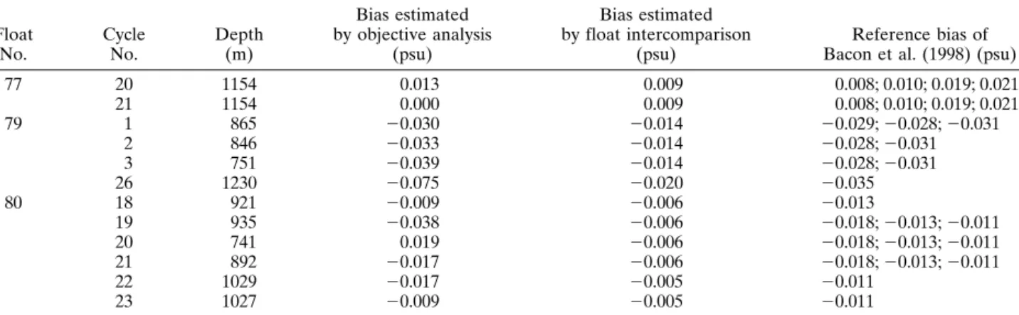
a. Comparison of our estimates with reference data The first validation step is to assess for floats 77, 79, and 80 the consistency between our estimates of the biases and independent estimates based on float– shipborne CTD comparisons by Bacon et al. (1998). These latter estimates are particularly well defined and are selected from a larger set of floats deployed in Oc-tober 1996 in the Irminger Sea. The comparisons Table 1) are presented for the 3.1°C iso- level, the deepest level sampled by the bulk of our dataset, where the space–time variability of the salinity field is lowest and hence where our bias estimates should be most reliable.
There is a reasonable consistency between the esti-mates using the different methods, with correlation and root-mean-square difference (rmsd) between the objec-tive analysis method and the reference biases of 0.78 and 0.022 psu, respectively. For the estimates derived by the intercomparison method, the correlation and rmsd with respect to the reference biases are 0.97 and 0.011 psu, respectively. The correlation and rmsd be-tween the estimates provided by the two algorithms are 0.86 and 0.026 psu, respectively. This rmsd of 0.026 psu is, however, rather large compared to the accuracy tar-geted for the bias estimation. An interesting diagnostic is the average bias estimated by the various approaches on this subset of the data. It is ⫺0.010 psu for the ref-erence biases of Bacon et al. (1998). The objective analysis method yields a⫺0.020 psu average bias. This large underestimation is likely linked to the Levitus climatology we use as a first guess of the analyzed sa-linity field. Indeed, 1996–97 corresponds to a fresh peak of the long-term salinity variations of the water mass sampled by our dataset. Over this period, the guess field will be influenced by the Levitus climatology, which is saltier, so that the mapped field will remain too salty, resulting in an estimated bias that is too negative. The intercomparison method, on the other hand, gives a negative average bias of⫺0.007 psu. This slight over-estimation of the bias (by 0.003 psu) suggests that there is a small negative bias of the whole dataset not taken into account, suggestive of an effect of biofouling. b. Overall comparison of the two approaches
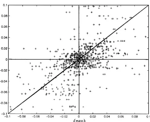
Figure 2 is a scatter diagram presenting the biases estimated on the 3.1°C iso- level for the whole dataset, obtained by both the objective analysis method and the float intercomparison method. The cluster of data along the y⫽ x axis is not very tight, with a correlation coefficient of 0.81 between the two classes of estimates. The objective analysis method presents a slight ten-dency to have smaller biases with respect to the inter-comparison method, with a mean absolute value of the estimated bias of 0.035 and 0.040 psu for the former
and for the latter, respectively. The standard deviation of the estimated bias is 0.060 psu for the objective analysis method and 0.064 psu for the intercomparison method.
Table 2 presents the results we obtained by the two methods in typical cases of high quality salinity data [float 78, which is one of the floats extensively validated by Bacon et al. (1998)] and of manifestly poor quality salinity data (float 678). According to both methods, float 78 presents small biases, weakly scattered. The standard deviation of the bias estimates remains within the bound of the nominal sensor accuracy of 0.008 psu. As for float 678, both methods are consistent in that there are large biases in the salinity data, predomi-nantly negative and markedly scattered (this is consis-tent with some biofouling happening for that sensor). This large scatter might suggest that the estimates are not very accurate for that float. Indeed, there is a large difference between the mean (⫺0.11 psu) and the me-dian (⫺0.17 psu) of the estimated biases, without being certain to which the real one should be closer.
5. Discussion and conclusions a. Discussion
We had some suggestions that the two methods tested provide fairly reasonable estimates of the biases, based on three floats that had been independently compared to CTD data. These estimates are consistent with the error estimates that the methods produce. However, this set of comparison is very limited geo-graphically and needs to be supported by further evi-dence. Thus, we decided to carry two additional com-parisons (here presented for the intercomparison method). The first one was to compare dynamic heights from the floats to altimetric sea level. The magnitude of the salinity biases estimated by the two methods (0.06 psu) is large and could induce large changes in verti-cally integrated dynamic height (0.06 psu over 1000 m roughly corresponds to a 6-cm difference). Therefore, one expects that this could make a difference in the
TABLE1. Comparison between the biases estimated by the two methods and the reference biases computed by Bacon et al. (1998).
Float No. Cycle No. Depth (m) Bias estimated by objective analysis (psu) Bias estimated by float intercomparison (psu) Reference bias of Bacon et al. (1998) (psu)
77 20 1154 0.013 0.009 0.008; 0.010; 0.019; 0.021 21 1154 0.000 0.009 0.008; 0.010; 0.019; 0.021 79 1 865 ⫺0.030 ⫺0.014 ⫺0.029; ⫺0.028; ⫺0.031 2 846 ⫺0.033 ⫺0.014 ⫺0.028; ⫺0.031 3 751 ⫺0.039 ⫺0.014 ⫺0.028; ⫺0.031 26 1230 ⫺0.075 ⫺0.020 ⫺0.035 80 18 921 ⫺0.009 ⫺0.006 ⫺0.013 19 935 ⫺0.038 ⫺0.006 ⫺0.018; ⫺0.013; ⫺0.011 20 741 0.019 ⫺0.006 ⫺0.018; ⫺0.013; ⫺0.011 21 892 ⫺0.017 ⫺0.006 ⫺0.018; ⫺0.013; ⫺0.011 22 1029 ⫺0.017 ⫺0.005 ⫺0.011 23 1027 ⫺0.009 ⫺0.005 ⫺0.011
comparisons with altimetric sea level. This was done by removing a climatological dynamic height to estimates from individual profiles and referencing the TOPEX/ Poseidon (T/P) altimetric data to the period 1993–99. The climatological dynamic height was computed from Levitus et al. (1994) mean fields and is certainly not very appropriate. The rmsd between sea level anoma-lies from T/P and the profile data was reduced from 9.5 to 8.0 cm when the data were corrected from the esti-mated biases obtained by float intercomparison ap-proach.
The second test was a comparison of near-surface salinity data from thermosalinographs (TSGs) on board merchant vessels to the 15-m salinity from the PALACE floats. The surface thermosalinograph data are de-scribed in Reverdin et al. (2002). They have been vali-dated and corrected based on surface samples collected by observers on a regular basis. Nonetheless, the data
have remaining uncertainties that are at least on the order of 0.01 psu and can reach 0.05 psu when there are insufficient calibration data or the TSG did not work satisfactorily, primarily in the autumn. The TSG data are collected on the two vessels at a depth close to 5 m, whereas the uppermost level with reliable data from the PALACE profiles is reported at 15 m. This can induce differences due to vertical stratification, in particular in late spring and summer. When comparing the data, care is taken that the temperature difference is not too large and that the data are reasonably close, in order to be sure to eliminate situations with very different water masses. For separations less than 25 km and 10 days, including data for all seasons and with temperature dif-ferences less than 0.75°C (27 data), the average differ-ence is 0.020 (PALACE saltier) with an rmsd of 0.060 psu. For the winter profiles, and with a larger distance of 50 km, the average difference is 0.003 with an rmsd
TABLE2. Examples of the biases estimated by the two methods for (a) a high quality float (78) and (b) a poor quality float (678).
a) Bias estimation method
No. of observations Average salinity bias (psu) Bias standard deviation (psu) Median bias (psu) Objective analysis 34 0.0028 0.0070 0.0017 Float intercomparison 30 ⫺0.0006 0.0063 0.0005
b) Bias estimation method
No. of observations Average salinity bias (psu) Bias standard deviation (psu) Median bias (psu) Objective analysis 26 ⫺0.1818 0.1862 ⫺0.2000 Float intercomparison 20 ⫺0.1177 0.1172 ⫺0.1715
FIG. 2. Comparison between the salinity biases estimated by the objective analysis method (horizontal) and by the intercomparison method (vertical) on the 3.1°C iso-level.
of 0.045 psu (23 data). The summer data are more scat-tered, with a positive bias suggestive of the occurrence of surface freshening. These results are reported for the PALACE data corrected from the biases estimated by the intercomparison method. However, results are fairly similar with the other method and are insignifi-cantly better than the ones without the corrections, the most noticeable differences being with a few data that were considered erroneous before the corrections and were not included in the comparisons. We also find that most of the profiler data included in the comparison with the TSG data are from floats for which the bias estimates are small. Because there might be additional errors in the near-surface PALACE data and because of the errors in the TSG data, the rmsd we find is prob-ably a fairly pessimistic estimate of the error on the corrected PALACE float salinity data.
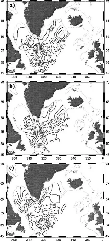
We wish now to assess the impact of correcting the data from the estimated biases onto the hydrological structure of the area. Figure 3 presents the average salinity field mapped onto the 3.1°C iso- level, for the raw data and for the data calibrated by the two methods we presented. One can see that the main effect of the bias correction is to smooth the spatial patterns. This is particularly noticeable in the case of the data corrected by float intercomparison. Notably, the raw data exhibit two fresh blobs at the southern edge of the domain between 45° and 50°N, with rather unrealistic values as low as 34.74 psu (Fig. 3a). The data corrected by the objective analysis method still exhibit these fresh pat-terns; however, they are clearly modified by the correc-tion, with values remaining above 34.78 psu (Fig. 3b). Interestingly, the data corrected by the float intercom-parison exhibit no salinity minimum in this area. In this case, this is a favorable feature of the method. In other areas, the tendency of the intercomparison method to reduce features might be detrimental (e.g., near the Greenland slopes). It would be possible to reduce this defect by removing an expected field (e.g., a climatol-ogy) from the data Obsijand the differences Dijbefore
applying the algorithm.
The preceding comments on the average field should also apply to the salinity fields for specific periods. As explained in section 2, the data coverage is representa-tive of ARGO recommendations only during 1997. Hence we now focus on this period and present the instantaneous salinity field on the 3.1°C iso- level for the July–August 1997 time step after correcting the bi-ases from the intercomparison method (Fig. 4). Just as in the case of the average salinity field, the impact of the correction on the unrealistic fresh blobs situated between 45° and 50°N is fine, with values everywhere superior to 34.86 psu in the corrected dataset. In the same way, it is interesting to notice that the freshwater (salinity less than 34.70 psu) visible in the raw data in the northeastern part of the domain around 57°N, 32°W (Fig. 4a) has been corrected to salinity greater than
34.82 psu. This latter value is much more consistent with the study of Bersch et al. (1999, their Fig. 9).
Finally, it is interesting to illustrate the impact of the estimated correction onto the hydrological structure of the whole water column sampled by the floats. To do
FIG. 3. Average salinity distribution on the 3.1°C iso-level for (a) the raw data, (b) the data corrected by the objective analysis method, and (c) the data corrected by the intercomparison method. Contour interval is 0.02 psu for (a) and (b) and 0.005 psu for (c). Isohalines below 34.86 psu are dashed.
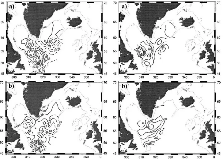
so, we applied to the whole profile the bias correction estimated via the float intercomparison method on the deepest available iso- levels, 3.1°, 3.3°, and 3.5°C. Then we computed the isopycnal surfaces depths for both the raw and corrected datasets. Figures 5 and 6 present the resulting field at a deep level (1⫽ 32.38)
and at a shallower level representative of the ther-mocline depth (1⫽ 32.30), respectively. On the deep
level (Fig. 5), both the raw and the corrected dataset exhibit an upward doming of the isopycnal surface, with minimal depth in the gyre interior around 55°N, 45°W and maximal depth at the edges. This is consistent with the known large-scale cyclonic circulation of the area (Lavender et al. 2000; Cuny et al. 2002). However, it is important to notice that the bias correction deepens the isopycnal surface in this region, again more consistently with the hydrological data from the cruises in 1997 (Bersch et al. 1999). As for the depth of the shallow isopycnal surface (Fig. 6), a major impact of the bias correction is smoothing of the small-scale patterns vis-ible in the raw data. Just as for the deep isopycnal depth, both the raw and corrected datasets exhibit a
doming structure. However, the maximum depth ex-ceeding 1100 m present in the raw data around 47°N, 45°W, and very likely caused by biases in the salinity data, is neatly lifted by the bias correction to a level around 800 m.
Further validation work would be to systematically compare the float profiles to the CTD data available mainly in 1996 and 1997.
b. Conclusions
In this study, we implemented two least squares– based methods to estimate salinity biases of an ARGO-type autonomous Lagrangian profiling float ensemble. The first method relies on an objective mapping of the data of the whole fleet. The second one consists of an intercalibration of the data by a least squares approach. Both methods were validated by checking their consis-tency with independent reference datasets. Also, they appear consistent with each other. However, we argue that the intercomparison method (section 3b) is slightly more reliable than the objective analysis method
(sec-FIG. 4. Salinity distribution in Jul–Aug 1997 on the 3.1°C iso- level for (a) the raw data and (b) the data corrected by the inter-comparison method. Contour interval is 0.04 psu for (a) and 0.01 psu for (b). Isohalines below 34.86 psu are dashed.
FIG. 5. Depth of the iso-1surface 32.38 in Jul–Aug 1997 for (a)
the raw data and (b) the data corrected by the intercomparison method. Contour interval is 200 m.
tion 3a). The corrections we estimated, once applied to the whole dataset, have a major impact on the hydro-logical structure retrieved from the float profiles, both at depth and in the main thermocline. With respect to the raw data, the corrected data are more consistent with the previous descriptions of the area made from ship cruises (Bersch et al. 1999; Reverdin et al. 2002). The salinity bias correction on the dynamic height anomaly retrieved from this dataset results in a signifi-cant improvement of the consistency with TOPEX/ Poseidon sea level variability. Eventually, the compari-son of corrected data with merchant vessel TSG data illustrated the absence of major systematic biases in the dataset. The methods could still be further improved by taking into account the inhomogeneity of the signals, which differ greatly in intensity between the center of the gyre and its rim or the subpolar front. One should also include known anisotropy of the signal, taking into account, for example, the distance to large bathymetric structures (continental margins, Reykjanes Ridge, etc.) or to known salinity fronts. This will require further developments of the method.
We do not rely on ancillary data so that the approach
could be applied in near real time. This, however, would be very valuable to detect an average bias of the data that these methods cannot detect. We suspect that this will often remain the case in near–real time, for which the methods were detected. This work was con-ducted in a case study area with data coverage in agree-ment with ARGO recommendations. However, it should also prove valuable in regions where the data coverage is poorer, with the condition that the param-eters of the analysis be tuned accordingly (typically by increasing the space and time characteristics in the weight or correlation functions so as to focus on larger bias detection), and by removing an a priori guess of the large-scale salinity gradients before comparing the data. It should also be tested whether additional infor-mation from satellite altimetry could be used to con-strain further the salinity bias estimations.
Acknowledgments. This work was partly supported by Service Hydrographique et Océanographique de la Marine (SHOM). Much of this work was undertaken at Laboratoire d’Etudes en Géophysique et Océanogra-phie Spatiales, Toulouse, France, for the CORIOLIS/ MERCATOR projects. Support from this institution is greatly acknowledged. The ships-of-opportunity data are part of the Observatoire en recherche pour l’environnement SSS, with initial support by PNEDC. We are thankful to Gilles Larnicol (Collecte Localisa-tion Satellite, France) for his comparison to altimetric sea level data.
REFERENCES
Arbic, B. K., and W. B. Owens, 2001: Climatic warming of At-lantic intermediate waters. J. Climate, 14, 4091–4108. Bacon, S., L. Centurioni, and W. J. Gould, 1998: Evaluation of
profiling ALACE float performance. Southampton Ocean-ography Centre Internal Doc. 39, 72 pp.
——, ——, and ——, 2001: The evaluation of salinity measure-ments from PALACE floats. J. Atmos. Oceanic Technol., 18, 1258–1266.
Bersch, M., J. Meincke, and A. Sy, 1999: Interannual thermoha-line changes in the northern North Atlantic 1991–1996.
Deep-Sea Res., 46B, 55–75.
Bretherton, F. P., R. E. Davis, and C. B. Fandry, 1975: A tech-nique for objective analysis and design of oceanographic ex-periments applied to MODE-73. Deep-Sea Res., 23, 559–582. Clarke, R. A., J. R. N. Lazier, and I. Yashayaev, 2000: Labrador Sea water mass variability during the WOCE period. Report of the WOCE North Atlantic Workshop Rep. 169/2000, WOCE International Project Office, Southampton, United Kingdom, 53–56.
Cuny, J., P. B. Rhines, P. P. Niiler, and S. Bacon, 2002: Labrador Sea boundary currents and the fate of the Irminger Sea Wa-ter. J. Phys. Oceanogr., 32, 627–647.
Curry, R. G., M. S. McCartney, and T. M. Joyce, 1998: Oceanic transport of subpolar climate signals to mid-depth subtropical waters. Nature, 391, 575–577.
Davis, R. E., 1998a: Autonomous floats in WOCE. International
WOCE Newsletter, No. 30, WOCE International Project
Of-fice, Southampton, United Kingdom, 3–6.
——, 1998b: Preliminary results from directly measuring mid-FIG. 6. Same as Fig. 5, for the iso-1surface 32.30. Contour
interval is 100 m.
depth circulation in the tropical and South Pacific. J.
Geo-phys. Res., 103, 24 619–24 639.
Fischer, J., and F. A. Schott, 2002: Labrador Sea Water tracked by profiling floats—From the boundary current into the open North Atlantic. J. Phys. Oceanogr., 32, 573–584.
Freeland, H., 1997: Calibration of the conductivity cells on P-ALACE floats. U.S. WOCE Implementation Rep. 9, 64 pp. Lavender, K., R. E. Davis, and W. B. Owens, 2000: Mid-depth recirculation observed in the interior Labrador and Irminger seas by direct velocity measurements. Nature, 407, 66–69. ——, ——, and ——, 2002: Observations of open-ocean deep
con-vection in the Labrador Sea from subsurface floats. J. Phys.
Oceanogr., 32, 511–526.
Lazier, J. R. N., 1973: The renewal of Labrador Sea water.
Deep-Sea Res., 20, 341–353.
Levitus, S., T. P. Boyer, and J. Antonov, 1994: Interannual
Vari-ability of Upper Ocean Thermal Structure. Vol. 5, World Ocean Atlas 1994, NOAA Atlas NESDIS 5, 176 pp.
Pickart, R. S., D. J. Torres, and R. A. Clarke, 2002: Hydrography of the Labrador Sea during active convection. J. Phys.
Ocean-ogr., 32, 428–456.
Reverdin, G., F. Durand, J. Mortensen, F. Schott, H. Valdimars-son, and W. Zenk, 2002: Recent changes in the surface salin-ity of the North Atlantic subpolar gyre. J. Geophys. Res., 107, 8010, doi:10.1029/2001JC001010.
Talley, L. D., and M. S. McCartney, 1982: Distribution and circu-lation of Labrador Sea Water. J. Phys. Oceanogr., 12, 1189– 1205.
Wong, A. P. S., G. C. Johnson, and W. B. Owens, 2003: Delayed-mode calibration of autonomous CTD profiling float salinity data by⌰–S climatology. J. Atmos. Oceanic Technol., 20, 308–318.