Statistical detection and isolation of additive faults in linear time-varying systems
Texte intégral
Figure
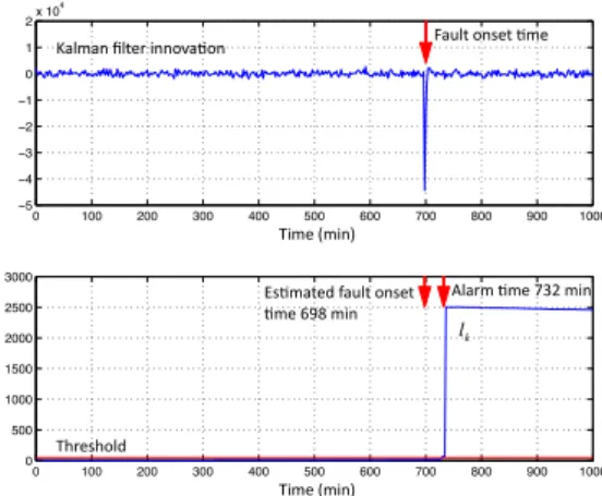
![Figure 4. Kalman filter innovation (Top) and GLR statis- statis-tics l k (Bottom) for the impulsive fault occurring at k = 201 with θ = [1.5, 0] T](https://thumb-eu.123doks.com/thumbv2/123doknet/12581505.346829/9.892.93.399.450.666/figure-kalman-filter-innovation-statis-statis-impulsive-occurring.webp)
Documents relatifs
The article is structured as follows: section 2 highlights some aspects on Bayesian networks and particularly on Bayesian network classifiers; section 3 presents the various T
Next, we used the conventional approach proposed by Pauly and Christensen (1995a) to estimate mean SPPRs of these species but using the mean transfer efficiency of 11.9%
Cette prédominance du corps de l’habitation toutefois ne doit pas nous rendre insensible à ces propos de Kenneth White : « Un monde c’est ce qui émerge du rapport entre
It is shown that the resulting technique, the Algorithmic Harmonic Balance- ρ ∞ (AHB-ρ ∞ ) method, can trace non-linear Frequency Response Functions (FRFs) of a time discretized
Moisture content (a) and Carbohydrate density (b): normalized variations introduced (solid) and neural network response (dashed) Using this neural network in untrained regions
Based on Lyapunov theory, two new approaches are proposed in term of Linear Matrix Inequalities (LMI) leading to synthesize an FTC laws ensuring the tracking between the reference
4(a,b) illustrates in low frequency the frequency of the fault (2fe) and in high frequency we note the presence of the frequency f MLI -2fe.The table below summarizes the results
The linear method performances are unsteady as the criterion fluctuates a lot (figure 5) and the most relevant frequency oscillates from one recording to another (figure 7), that may
