HAL Id: hal-01500459
https://hal.archives-ouvertes.fr/hal-01500459
Submitted on 3 Apr 2017
HAL is a multi-disciplinary open access
archive for the deposit and dissemination of
sci-entific research documents, whether they are
pub-lished or not. The documents may come from
teaching and research institutions in France or
abroad, or from public or private research centers.
L’archive ouverte pluridisciplinaire HAL, est
destinée au dépôt et à la diffusion de documents
scientifiques de niveau recherche, publiés ou non,
émanant des établissements d’enseignement et de
recherche français ou étrangers, des laboratoires
publics ou privés.
SHREC’17 Track: Point-Cloud Shape Retrieval of
Non-Rigid Toys
F. A. Limberger, R. C. Wilson, M. Aono, N. Audebert, A. Boulch, B. Bustos,
A Giachetti, A. Godil, B. Le Saux, B. Li, et al.
To cite this version:
F. A. Limberger, R. C. Wilson, M. Aono, N. Audebert, A. Boulch, et al.. SHREC’17 Track:
Point-Cloud Shape Retrieval of Non-Rigid Toys. 10th Eurographics workshop on 3D Object retrieval, Apr
2017, Lyon, France. pp.1 - 11. �hal-01500459�
Eurographics Workshop on 3D Object Retrieval (2017), pp. 1–11 I. Pratikakis, F. Dupont, and M. Ovsjanikov (Editors)
SHREC’17 Track: Point-Cloud Shape Retrieval of Non-Rigid Toys
†
F. A. Limberger‡1, R. C. Wilson‡1, M. Aono6, N. Audebert9, A. Boulch7, B. Bustos7, A. Giachetti5, A. Godil13, B. Le Saux8, B. Li11, Y. Lu12, H.-D. Nguyen2,4, V.-T. Nguyen2,3, V.-K. Pham2, I. Sipiran8, A. Tatsuma6, M.-T. Tran2, S. Velasco-Forero10
1Univeristy of York, United Kingdom,2University of Science, VNU-HCM, Vietnam,3University of Information Technology, VNU-HCM, Vietnam, 4John von Neumann Institute, VNU-HCM, Vietnam,5University of Verona, Italy,6Toyohashi University of Technology, Japan,
7Dept. Computer Science, University of Chile, Chile,8Dept. Engineering, Pontifical Catholic University of Peru, Peru, 9ONERA, The French Aerospace Lab, France,10Centre de Morphologie Mathématique, MINES Paristech, France, 11University of Southern Mississippi, USA,12Texas State University, USA,13National Institute of Standards and Technology, USA
Abstract
In this paper, we present the results of the SHREC’17 Track: Point-Cloud Shape Retrieval of Non-Rigid Toys. The aim of this track is to create a fair benchmark to evaluate the performance of methods on the non-rigid point-cloud shape retrieval problem. The database used in this task contains 100 3D point-cloud models which are classified into 10 different categories.
All point clouds were generated by scanning each one of the models in their final poses using a 3D scanner, i.e., all models
have been articulated before scanned. The retrieval performance is evaluated using seven commonly-used statistics (PR-plot, NN, FT, ST, E-measure, DCG, mAP). In total, there are 8 groups and 31 submissions taking part of this contest. The evaluation results shown by this work suggest that researchers are in the right way towards shape descriptors which can capture the main characteristics of 3D models, however, more tests still need to be made, since this is the first time we compare non-rigid signatures for point-cloud shape retrieval.
Categories and Subject Descriptors(according to ACM CCS): H.3.3 [Computer Graphics]: Information Systems—Information
Search and Retrieval
1. Introduction
With the rapid development of virtual reality (VR) and augmented reality (AR), especially in gaming, 3D data has become part of our everyday lives. Since the creation of 3D models is essential to these applications, we have been experiencing a large growth in the num-ber of 3D models available on the Internet in the past years. The problem now has been organizing and retrieving these models from databases. Researchers from all over the world are trying to create shape descriptors in a way to organize this huge amount of models, making use of many mathematical tools to create discriminative and efficient signatures to describe 3D shapes. The importance of shape retrieval is evidenced by the 11 years of the Shape Retrieval Contest (SHREC).
There are two distinct areas which concern shape retrieval: The first, non-rigid shape retrieval, which deals with the problem
of articulations of the same shape [LGT∗10,LGB∗11,LZC∗15],
and second, comprehensive shape retrieval [BBC∗10,LLL∗14,
SYS∗16], which deals with any type of deformation, for example,
scaling, stretching and even differences in topology. While compre-hensive shape retrieval is more general, non-rigid shape retrieval is
† Website: https://www.cs.york.ac.uk/cvpr/pronto ‡ Track organizers. E-mail: pronto-group@york.ac.uk
as important when it is necessary to carefully classify similar ob-jects that are in distinct classes [PSR∗16].
Three-dimensional point clouds are the immediate result of scans of 3D objects. Although there are efficient methods to create meshes from point clouds, sometimes this task can be complex, particularly when point-cloud data present missing parts or noisy surfaces, for example, fur or hair. In this paper, we are interested in the non-rigid shape retrieval task, therefore we propose to create a non-rigid point-cloud shape retrieval benchmark (PRoNTo: Point-Cloud Shape Retrieval of Non-Rigid Toys), which was produced given the necessity of testing non-rigid shape signatures computed directly from unorganized point clouds, i.e., without any connec-tivity information. This is the first benchmark ever created to test, specifically, the performance of non-rigid point-cloud models.
This benchmark is important given the need to compare 3D non-rigid shapes based directly on a rough 3D scan of the object, which is a more difficult task than comparing signatures computed from well-formed 3D meshes. 3D scanners may introduce some sam-pling problems to the scanned models, given the difficulty of reach-ing all parts of the object by the scan head and given that some materials have specular properties and these can generate outliers.
Although some methods available in the literature use point sets to create their shape signatures, we have not seen these methods
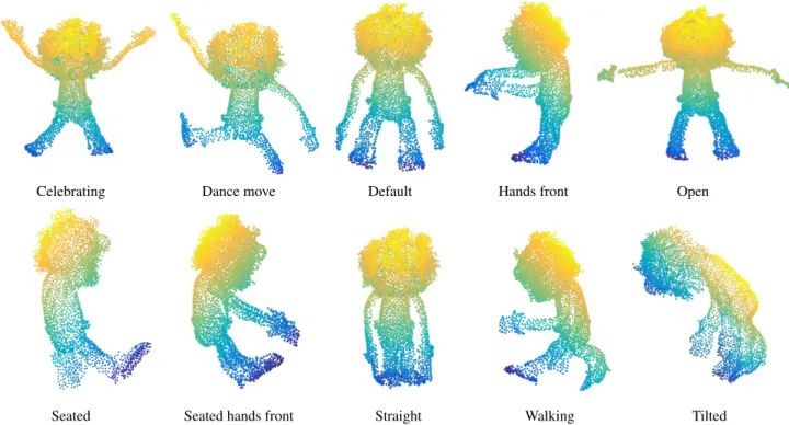
Celebrating Dance move Default Hands front Open
Seated Seated hands front Straight Walking Tilted
Figure 1: Different poses captured of the objects, showing model Monster as an example. Point clouds were coloured by Y and Z coordinates.
being used directly to address the non-rigid point-cloud shape-retrieval problem since there are no specific point-cloud datasets available for this purpose. Instead, these methods normally use mesh vertices, which sometimes can be a very bad idea, unless ver-tices are very well distributed along the surface of the shape.
2. Dataset
Our dataset consists of 100 models that are derived from 10 dif-ferent real objects. Each real object was scanned in 10 distinct poses by phisically articulating them around their joints before be-ing scanned. The different poses and each one of the objects used to
create this database can be seen in Figures1and2, respectively.
Af-ter scanning all the poses we manually removed the supports used to scan the objects using MeshLab.
Objects were scanned using the Head & Face Color 3D Scan-ner of Cyberware. This scanScan-ner makes a 360 degrees scan around the object estimating x, y, and z coordinates of a vertical patch. The scanning process captures an array of digitized points and also the respective RGB colors although they are not used in this con-test. The file format for the objects was chosen as the Object File Format (.off), which, in this case, contains only vertex informa-tion. We also resample models using the Poisson-Disk Sampling
algorithm [CCS12] since the scan generates an arbitrary number of
samples. This way, we control the sampling rate so that every model has approximately 4K points. Finally, we perform an arbitrary ro-tation of the model so that it is not always in the same orienro-tation.
The point clouds acquired by our scans suffer from common scanning problems like holes and missing parts resulted from
self-occlusions of the shapes, and also from noise given that some toy’s materials have specular properties. To avoid fine-tuning of param-eters, we have chosen relatively similar classes to be part of this dataset, therefore it would be cumbersome to identify classes just by looking at the point clouds shapes, for example, Teddy and Sheep or Fox and Dog.
Bear Dog Einstein Fox Monkey
Monster Rat Sheep Teddy Tiger
Figure 2: Different toys used to create the PRoNTo dataset. 3. Evaluation
The evaluation rules follow standard measures used in SHREC tracks in the past. We asked participants to submit up to 6
dis-D. Fellner & S. Behnke / SHREC’17 Track: Point-Cloud Shape Retrieval of Non-Rigid Toys 3
similarity matrices. These matrices could be the result of differ-ent algorithms or differdiffer-ent parameter settings, at the choice of the participant. A dissimilarity matrix is the result of a shape retrieval problem which gives the difference between every model in the database. It has the size N × N, where N is the number of models of the dataset and the position (i, j) in the matrix gives the differ-ence between models i and j. No class information is provided with the data, and supervised methods are not allowed in the track.
In total, seven standard quantitative evaluation measures were computed over the dissimilarity matrices submitted by the partic-ipants to test the retrieval accuracy of the algorithms: Precision-and-Recall (PR) curve, mean Average Precision (mAP), E-Measure (E), Discounted Cumulative Gain (DCG), Nearest Neighbor (NN), First-Tier (FT) and Second-Tier (ST).
4. Participants
During this contest, we had 8 groups taking part in the SHREC’17 PRoNTo contest and we received in total 31 dissimilarity-matrix submissions, as detailed below:
1. MFLO-FV-IWKS, MFLO-SV-IWKS, FV-IWKS, PCDL-SV-IWKS, GL-FV-IWKS and GL-SV-IWKS submitted by Fred-erico A. Limberger and Richard C. Wilson.
2. 1, 2, DMF-3, BoW-RoPS-DMF-4, BoW-RoPS-DMF-5 and BoW-RoPS-DMF-6 submitted by Minh-Triet Tran, Viet-Khoi Pham, Hai-Dang Nguyen and Vinh-Tiep Nguyen. Other team members: Thuyen V. Phan, Bao Truong, Quang-Thang Tran, Tu V. Ninh, Tu-Khiem Le, Dat-Thanh N. Tran, Ngoc-Minh Bui, Trong-Le Do, Minh N. Do and Anh-Duc Duong.
3. POHAPT and BPHAPT submitted by Andrea Giachetti. 4. CDSPF submitted by Atsushi Tatsuma and Masaki Aono.
5. SQFD(HKS), SQFD(WKS), SQFD(SIHKS),
SQFD(WKS-SIHKS)and SQFD(HKS-WKS-SIHKS) submitted by Benjamin
Bustos and Ivan Sipiran.
6. SnapNet submitted by Bertrand Le Saux, Nicolas Audebert and Alexandre Boulch.
7. AlphaVol1, AlphaVol2, AlphaVol3 and AlphaVol4 submitted by Santiago Velasco-Forero.
8. m3DSH-1, m3DSH-2, m3DSH-3, m3DSH-4, m3DSH-5 and
m3DSH-6submitted by Bo Li, Yijuan Lu and Afzal Godil.
5. Methods
In the next sections, we detail all the participant methods that have successfully competed in the PRoNTo dataset contest. Experimen-tal settings of each method are displayed at the end of each section.
5.1. Spectral Descriptors for Point Clouds, by Frederico Limberger and Richard Wilson
The key idea of this method is to test spectral descriptors computed directly from point clouds using different formulations for the com-putation of the Laplace-Beltrami operator (LBO). We test three dif-ferent methods for computing the LBO: the Mesh-Free Laplace
op-erator (MFLO), the Point-Cloud Laplace (PCDLaplace) [BSW09]
and the Graph Laplacian (GL).
Our framework is as follows. We first compute the eigendecom-position of the different LBO methods. Then, we compute local descriptors. We encode these local features using state-of-the-art encoding schemes (FV and SV). Furthermore, we compute the dif-ferences between shape signatures using Efficient Manifold Rank-ing. We now detail each part of our framework.
Laplace-Beltrami operator: The LBO is a linear operator defined as the divergence of the gradient, taking functions into functions over the 2D manifold M
∆Mf= − 5 · 5Mf (1)
given that f is a twice-differentiable real-valued function. Although we compute the LBO using three different methods, all these use the same parameters that are equivalent in each approach. The eigendecomposition of the LBO results in their eigenvalues and eigenfunctions, which are commonly known as the shape spectrum and these are further used to compute a local descriptor.
Local Descriptor: After computing the shape spectrum, we
com-pute the Improved Wave Kernel Signature (IWKS) [LW15] which
is a local spectral descriptor based on the Schrodinger equation and it is governed by the wave function ψ(x,t).
i∆Mψ(x, t) =∂ψ
∂t(x,t), (2)
The IWKS is an improved version of the WKS [ASC11]. It has a
different weighting filter of the shape spectrum which captures, at the same time, the major structure of the object and its fine details, therefore being more informative than the WKS.
Encoding: For computing the encoding of local descriptors into global signatures for shape retrieval, we use state-of-the-art
encod-ings: Fisher Vector (FV) [PD07] and Super Vector (SV) [ZYZH10].
These methods are based on the differences between descriptors and probabilistic distribution functions, which we approximate by Gaussian Mixture models. More details about these encodings can
be found in [LW15].
Distances between signatures: Distances between signatures are
computed using Efficient Manifold Ranking (EMR) [XBC∗11],
which accelerates the classic Manifold Ranking [ZWG∗04]. EMR
has similar evaluation performance to MR, however, it has much lower computation times when used in large databases.
Experimental settings: We compute the first 100 eigenvalues and eigenfunctions of the respective LBO using 15 nearest neighbours to compute the proximity graph for all methods. In PCDLaplace, we use the following additional parameters: htype = ddr; hs = 2; rho = 2. For the computation of the local descriptor, we use
iwksvar= 5. For computing the Gaussian dictionary, we use the
first 29 models of the database to create GMMs with 38 compo-nents for each signature frequency. For computing EMR we use 99 landmarks and we use k-means as the landmark selection method. The number of landmarks is usually chosen as a slightly smaller number than the number of models in total. For one model in the database, it takes approximately 15 seconds to compute the MFLO-IWKS, 8 seconds to compute the GL-IWKS and 11 seconds to compute the PCDL-IWKS. To compute the entire dissimilarity ma-trix it takes approximately 43 seconds with the FV and 56 seconds
Vertex Selection Uniform sampling . .. . . . . . . . . . . . . . . .. . . . ... ... ... .. . ... ... ... ... . . .... .... .. . . . .. . . . . .... ... .. . . . . . . . . . . .... . .. ... . . . . . . . . . ... .. ..... . . . .. ... ... .. . . . . . . . . . . . .. Feature Description Point- cloud-based RoPS n CodebookTraining Approximate K-means tf-idf weighting Soft assignment . . . . . . . . … Point-cloud-Word Vectors Point-cloud Word Vocabulary Quantization
Selected Vertices Feature Descriptors
Inverted index tree I 3D Model Indexing Feature Encoding
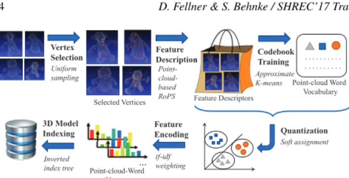
Figure 3: Bag-of-Words framework for 3D object retrieval
with the SV. All experiments were carried out in Matlab on a PC CPU i7-3770 3.4GHz, 8GB RAM.
5.2. Bag-of-Words Framework for 3D Object Retrieval, by Minh-Triet Tran, Viet-Khoi Pham, Hai-Dang Nguyen and Vinh-Tiep Nguyen
We develop our framework for 3D object retrieval based on
Bag-of-Words scheme for visual object retrieval [SZ03]. BoW method
originated from text retrieval domain and is shown to be
success-fully applied on large-scale image [NNT∗15] and 3D object
re-trieval [PSA∗16]. Figure3illustrates the main components of our
framework.
Preprocessing: Each point cloud is normalized into a unit cube and densified to reduce significant difference in the density between different parts.
Feature detector: For each model, we uniformly take random
sam-ples of 5% ≤ pSampling≤ 50%.
Feature descriptor: We describe the characteristics of the point cloud in a sphere with supporting radius r surrounding a selected vertex. We propose our point-cloud-based descriptor inspired by
the idea of RoPS [GSB∗13] to calculate the descriptor directly from
a point cloud (without reconstructing faces). We first estimate the eigenvectors of the point cloud within a supporting radius r of a selected vertex, then transform the point cloud to achieve rotation invariant for the descriptor, and finally calculate the descriptor. We consider the supporting radius r from 0.01 to 0.1.
Codebook: All features extracted from the models are used to build a codebook with size relatively equal to 10% of the total number of features in the corpus, using Approximate K-Means.
Quantization: To reduce quantization error, we use
soft-assignment [PCI∗08] with 3 nearest neighbors.
Distance measure metric: instead of using a symmetric distance,
we use L1, asymmetric distance measurement [ZJS13], to evaluate
the dissimilarity of each pair of objects.
Our first two runs (1 and 2) are results of our BoW framework
using random sampling with pSampling= 45% and codebook size
of 18000. The radius of point-cloud based RoPS for run 1 and 2 are
r= 0.04 and 0.05, respectively.
Each main component of our BoW framework is deployed on a
different server. Codebook training module using Python 2.7 is de-ployed on Ubuntu 14.04 with 2.4 GHz Intel Xeon CPU E5-2620 v3, 64 GB RAM. It takes 30 minutes to create a codebook with 18,000 visual words from 180,000 features. 3D feature extraction and de-scription module, written in C++, runs on Ubuntu 14.04, 2GHz In-tel Xeon CPU E5-2620, 1GB RAM.
The retrieval process in Matlab R2012b with feature quantization and calculating the dissimilarity matrix is performed on Windows Server 2008 R2, 2.2GHz Intel Xeon CPU E5-2660, 12 GB RAM. The average time to calculate features of a model is 1-2 seconds and it takes on average 0.02 seconds to compare an object against all 100 objects.
5.2.1. Distance Matrix Fusion
With each setting for our BoW framework, we get a different re-trieval model. We propose a simple method to linearly combine k distance matrices D1, D2, ..., Dk with different coefficients into a new distance matrix:
DFusion= w1D1+ w2D2+ ...wkDk. (3)
Our objective is to take advantage of different retrieval models obtained from our framework with the expectation to increase the performance of the retrieval process.
We limit the number of seeds k of 2 or 3, and the value of a
coefficient wiis from 0 to 1, step 0.2. Our last four runs are
com-binations of Run1 and Run2 with different values of w1and w2:
Run3: w1= 0.8 and w2 = 0.6; Run4: w1= 1.0 and w2 = 0.8;
Run5: w1= 0.6 and w2= 0.2; and Run6: w1= 1.0 and w2= 0.4.
Experimental results show that the fusion runs can even yield better performance in retrieval than the two original seeds.
5.3. Simple meshing and Histogram of Area Projection Transform, by Andrea Giachetti
The method is based on simple automatic point cloud meshing fol-lowed by the estimation of the Histogram of Area Projection
Trans-form descriptor [GL12]. Shapes are represented through a set of N
voxelized maps encoding the area projected along the inner normal
direction at sampled distances Ri, i = 1..N in a spherical
neighbor-hood of radius σ around each voxel center location ~x. Values at dif-ferent radii are weighted in order to have a scale-invariant behavior. Histograms of MAPT computed inside the objects are quantized in 12 bins and evaluated at 12 equally spaced radii values rang-ing from 3 to 39mm., with σ always taken as half the radius. His-tograms computed at the different radii considered are concatenated creating an unique descriptor. Dissimilarity matrices are generated by measuring the histogram distances with the Jeffrey divergence.
This descriptor is robust against pose variation and inaccuracy due to holes, especially if histograms are estimated inside the shape only. For this reason we applied the HAPT estimation using the code publicily available at the web site www.andreagiachetti.it on closed meshes estimated on the original point clouds with two
different procedures implemented as simple Meshlab [CCC∗08]
scripts.
We submitted matrices corresponding to each of these proce-dures.
D. Fellner & S. Behnke / SHREC’17 Track: Point-Cloud Shape Retrieval of Non-Rigid Toys 5
Poisson reconstruction: In the first run, we just applied Poisson
reconstruction [KBH]. Points’ normals have been estimated on a
12 neighbors range, and the octree depth has been set equal to 9. Ball Pivoting and Poisson: In the second run we first smoothed the point set using Moving Least squares, then we applied the ball
pivoting method [BMR∗99] to extract an open mesh. The mesh
has been refined with triangle splitting and normals have been re-computed on the basis of the meshing. From mesh and normals obtained, a closed watertight mesh has been finally obtained with the Poisson reconstruction method.
Note that meshing would be not mandatory for the application of the method, as a point cloud implementation of the descriptor would be quite simple. However, we believe that Poisson meshing provides in general a better estimate of the inner part of the mesh and is effective in reconstructing missing parts in a reasonable way. Meshlab scripts runs in less than one second per model and HAPT estimation takes 10 seconds on average. Histogram distance estimation time, performed in Matlab, is negligible in comparison.
5.4. Covariance Descriptor with Statistics of Point Features, by Atsushi Tatsuma and Masaki Aono
For non-rigid human 3D model retrieval, we previously proposed
the local feature extraction method [PSR∗16] that calculates the
histogram, mean, and covariance of geometric point features. In this track, we further calculate the skewness and kurtosis of geo-metric point features to obtain more discriminative local feature. 3D point-cloud object finally is represented with the covariance of the local features consisting of the histogram, mean, covariance, skewness, and kurtosis of geometric point features. We call our ap-proach the Covariance Descriptor with Statistics of Point Features (CDSPF).
The overview of our approach is illustrated in Figure4. We first
calculate 4D point geometric feature f = [ f1, f2, f3, f4] proposed
in [WHH03]. The geometric feature is computed for every pair of
points paand pbin the point’s k-neighborhood:
f1 = tan−1(w · nb/u · na), (4)
f2 = v · nb, (5)
f3 = u · (pb− pa/d), (6)
f4 = d, (7)
where the normal vectors of paand pbare naand nb, u = na, v =
(pb− pa) × u/||(pb− pa) × u||, w = u × v, and d = ||pb− pa||. Next, we collect the point features in a 16-bin histogram h. The index of histogram bin h is defined by the following formula:
h=
4
∑
i=1
2i−1s(t, fi), (8)
where s(t, f ) is a threshold function defined as 0 if f < t and 1
otherwise. The threshold value used for f1, f2 and f3 is 0, while
the threshold value for f4 is the average value of f4 in the
k-neighborhood.
Furthermore, we calculate the mean, covariance matrix, skew-ness, and kurtosis of the point features. Let f1, f2, . . . , fNbe the point
!"! !#! $%&'()*+,-.(/0& (123-+& 43(53+6)-& '()*+&!37+/638& )*&.(-7.&639)(*& :+7;8;-8&(!& '()*+&!37+/638& <.(-7.&!37+/63=& >(?76)7*-3& 038-6)'+(6&@)+A& +A3&83+&(!&.(-7.& !37+/638& Figure 4: Overview of CDSPF extraction process.
features of size N. The mean µ, covariance matrix C, skewness s,
and kurtosis k are calculated as follows [Mar70]:
µ = 1 N N
∑
i=1 fi, (9) C = 1 N N∑
i=1 (fi− µ)(fi− µ)>, (10) s = 1 N2 N∑
i=1 N∑
j=1 {(fi− µ)>C−1(fi− µ)}3, (11) k = 1 N N∑
i=1 {(fi− µ)>C−1(fi− µ)}2. (12)Since the covariance matrix C lies on the Riemannian manifold of symmetric positive semi-define matrices, we map the covariance matrix onto a point in the Euclidean space by using Pennec et al.’s
method [PFA06].
We finally obtain the local feature by concatenating the his-togram, mean, covariance, skewness, and kurtosis of the point fea-tures. The local feature is normalized with the signed square rooting
and `2normalization [JC12]. To compare 3D point-cloud objects,
we integrated the set of local features into a feature vector with the
covariance descriptor approach [TPM06].
Since 3D point-cloud objects in the dataset do not have normal
vector information, we used the Point Cloud Library [RC11] for
estimating normal vector of each point. Moreover, we set the size of the neighborhood k to 30. We employ the Euclidean distance for the dissimilarity between two feature vectors.
The method was implemented in C++. Experiments were carried out under Debian Linux 8.7 on a CPU 3.4GHz Intel Core i7-6800K and 128GB DDR4 memory. The average time to calculate the shape descriptor for a 3D model is about 1.46 seconds and it takes approx-imately 10 seconds to compute the dissimilarity matrix.
5.5. Signature Quadratic Form Distance on Spectral Descriptors, by Ivan Sipiran and Benjamin Bustos Our method combines the flexibility of the Signature Quadratic
Form Distance (SQFD) [BUS09] with the robustness of
intrin-sic spectral descriptors. On the one hand, the SQFD distance has proven to be effective in multimedia domains where objects are
represented as a collection of local descriptors [SLBS16]. On the
other hand, intrinsic descriptors are useful to keep robustness to non-rigid transformations. Our proposal consists of representing
the input 3D point cloud as a set of local descriptors which will be compared through the use of the SQFD distance.
Let P be a 3D point cloud. The first step of our method is to compute a set of local descriptors on P. The spectral descriptors depends on the computation of the Laplace-Beltrami operator on the point cloud. So a pre-processing step is needed to guarantee a proper computation of this operator. The pre-processing is per-formed as follows
• Normal computation. We compute a normal for each point in the point cloud. For a given point, we get the 20 nearest neigh-bors and compute the less dominant direction of the neighbor-hood.
• Poisson reconstruction. We reconstruct the surface for the point
cloud using the screened Poisson reconstruction method [KH13].
We set the octree depth to eight and the depth for the Laplacian solver to six. The output is a Manifold triangle mesh that pre-serves the structure of the original point cloud.
Let M be the obtained mesh. We compute a local descriptor for each vertex in the mesh. We denote the set of local descriptors of
the mesh M as FM. The challenge now is how to compare two
ob-jects through their collections of local descriptors. The approach to use the SQFD distance establishes that we need to compute a more compact representation called signature. Let suppose the existence
of a local clustering on FM that groups similar local descriptors
such that the number of clusters is n and FM= C1TC2T. . .Cn.
The signature is defined as SM= {(cMi , wMi ), i = 1, . . . , n}, where cMi = ∑d∈Cid
|Ci| and w
M
i =
|Ci|
|FM|. Each element in the signature
con-tains the average descriptor in the cluster (cMi ) and a weight (wMi ) to quantify how representative is the cluster in the collection of lo-cal descriptors.
Note that the local clustering is a key ingredient of the compu-tation of the signatures. Here we briefly give some details about the clustering. We use an adaptive clustering method that searches groups of descriptors using two distance thresholds. The method uses an intra-cluster threshold λ that sets the maximum distance between descriptors in the same cluster. Also, the method uses an inter-cluster threshold β that sets the minimum distance between centroids of different clusters. In addition, the clustering method only preserves clusters with a number of descriptors greater than a
parameter Nm. More details can be found in [SLBS16].
Given two objects M and N, and their respective signatures SM
and SN, the Signature Quadratic Form Distance is defined as
SQFD(SM, SN) =
q
(wM| − wN) · A
sim· (wM| − wN)T (13)
where (wA|wB) denotes the concatenation of two weight vectors.
The matrix Asimis a block similarity matrix that stores the
correla-tion coefficients between clusters. To transform a distance between cluster centroids to a correlation coefficient, we need to apply a similarity function. We use the Gaussian similarity function
sim(ci, cj) = exp(−αd2(ci, cj)). (14)
Note that to compute the transformation, we need to choose the value of parameter α and the ground distance for descriptors. In all
our experiments, we use α = 0.9 and L2as ground distance. More
details about the computation of signatures and the SQFD distance
can be found in [SLBS16].
Experimental Settings: We provide five runs using different con-figurations. Here, we describe the parameters used in each run • SQFD(WKS). We use the normalized Wave Kernel
Signa-ture [ASC11] as local descriptor. The parameters for local
clus-tering are λ = 0.2, β = 0.4, Nm= 30.
• SQFD(HKS). We use the normalized Heat Kernel
Signa-ture [SOG09] as local descriptor. The parameters for local
clus-tering are λ = 0.1, β = 0.2, Nm= 20.
• SQFD(SIHKS). We use the Scale-invariant Heat Kernel
Signa-ture [BK10] as local descriptor. The parameters for local
cluster-ing are λ = 0.1, β = 0.2, Nm= 20.
• SQFD(WKS-SIHKS). We use a distance function as a combina-tion of distances. For every pair of objects, we compute the sum of the distances obtained with SQFD(WKS) and SQFD(SIHKS). • SQFD(HKS-WKS-SIHKS). We use the combination of three distances. We use the weighted sum of distances SQFD(HKS), SQFD(WKS) and SQFD(SIHKS). The weights are 0.15, 0.15 and 0.7, respectively.
We implemented our method in Matlab under Windows 10 on a PC CPU i7 3.6 GHz, 12GB RAM. The average time to compute the shape signature for a 3D model is about 5 seconds and it takes approximately 0.3 seconds to compare a pair of signatures.
5.6. SnapNet for Dissimilarity Computation, by Alexandre Boulch, Bertrand Le Saux and Nicolas Audebert
The objective of this approach is to learn a classifier, in an unsu-pervised way, that will produce similar outputs for the same shapes with different poses. As we do not know the ground truth, i.e. the model used to generate the pose, we will train the classifier as if each pose was a different class. It is a 100-class problem.
Training dataset: The training dataset is generated by taking
snap-shots around the 3D model [Gra14]. In order to create visually
con-sistent snapshots, we mesh the point cloud using [MRB09]. The
snapshots are 3-channel images. The first channel encodes the dis-tance to the camera (i.e. depth map), the second is the normal orien-tation to the camera direction and the third channel is an estimation of the local noise in the point cloud (ratio of eigenvalues of the neighborhood covariance matrix). An example of such a snapshot is presented in Figure5(left).
CNN training: The CNN we train is a VGG16 [SZ14] with a last
fully connected layer with a 100 outputs. We initialize the weights with the model trained on the ILSVRC12 contest. We then finetune the network using a step learning rate policy.
Distance computation: The classifier is then applied to images
and produces images classification vectors vim. For each model we
compute a prediction vector VMbased on the images:
VM= ∑im∈M
vim || ∑im∈Mvim||2
D. Fellner & S. Behnke / SHREC’17 Track: Point-Cloud Shape Retrieval of Non-Rigid Toys 7
Figure 5: Snapshot example (left) and dissimilarity matrix (right).
The distance matrix X contains the pairwise `2distances between
the VM. Each line is then normalized using a soft max:
Xi, j=
exp(Xi, j) ∑jexp(Xi, j)
(16) Matrix X is not symmetrical. We finally define the symmetrical
distance matrix as D is such that D = XTX. The values of D are
clipped according to the 5thand 50thpercentiles and then re-scaled
in [0, 1]. The resulting matrix is presented on Figure5(right).
The method was implemented in Python and C++, using the deep learning framework Pytorch. We ran the experiments on Linux, CPU Intel Xeon(R) E5-1620 3.50GHz. The training part was op-erated on a NVidia Titan X Mawell GPU and the test part (pre-dictions) on a NVidia GTX 1070. Generating the snapshots took around 10 seconds per model. The training took around 8 hours. The prediction vectors were generated in 2 seconds per model and the dissimilarity matrix is computed in less than 10s.
5.7. Alpha-shapes volume curve descriptor, by Santiago Velasco-Forero
Given S be the set of finite set of points in R3, we have computed
a set of three-dimensional alpha-shapes of radius r, proposed by
Edelsbrunner [EM94], and denoted by αr(S). Rather than
find-ing an optimal fixed value, we focus on a range of values for the scale parameter r, and our descriptor computes the volume of each
αr(S). Thus, the similarity of two shapes is then computed by the
distance of their alpha-shapes volume curve in Euclidean norm. An
example of different αr(S) by varying r is illustrated in Figure6.
The values of parameter (r) used in the different submission are: • AlphaVol 1: r ∈ [0.02, 0.045, 0.07]
• AlphaVol 2: r ∈ [0.02, 0.045, 0.07, 0.095] • AlphaVol 3: r ∈ [0.02, 0.045, 0.07, 0.095, 0.12] • AlphaVol 4: r ∈ [0.02, 0.045, 0.07, 0.095, 0.12, 0.145]
We have implemented our method in Matlab and carried out ex-periments under Mac on a PC CPU Intel Core i7 2.8 GHz, 16 GB RAM 1600MHz DDR3, and a NVIDIA GeForce GT 750M 2048 MB. The average computation times for the shape descriptors are as follows: AlphaVol1: 92 ms, AlphaVol2: 108 ms, AlphaVol3: 118 ms and AlphaVol4: 137 ms and it takes approximately 1.48 seconds to compute the dissimilarity matrix in the four cases.
(a) vol(αr=0.005(S)) = 0.0001 (b) vol(αr=0.01(S)) = 0.0003 (c) vol(αr=0.035(S)) = 0.0025
Figure 6: Example of representation space by α-shapes 5.8. Modified 3D Shape Histogram for non-rigid 3D toy model
retrieval (m3DSH), by Bo Li, Yijuan Lu and Afzal Godil The 100 non-rigid point cloud toy models contain only 3D points to represent ten different poses for each of the ten toys. We can first reconstruct a 3D surface for each 3D point cloud such as to extract our previously developed 3D surface-based non-rigid shape descriptors. However, considering retrieval efficiency, the raw point cloud data is directly used for 3D shape descriptor extraction for shape comparison. For simplicity, we chose 3D Shape Histogram
(3DSH) [AKKS99]. The original 3DSH descriptor uniformly
par-titions the surrounding space of a 3D shape into a set of shells, sectors or spiderweb bins and counts the percentage of the surface sampling points falling in each bin to form a histogram as the 3DSH descriptor. Rather than like the original 3DSH descriptor which di-vides the space uniformly, to increase its descriptiveness we devel-oped a modified variation of 3DSH descriptor, that is m3DSH, by dividing the 3D space occupied by a 3D shape in a non-uniform way.
Figure7illustrates the overview of the feature extraction
pro-cess: Principal Component Analysis (PCA) [Jol02]-based 3D
model normalization, and extraction of a modified 3D Shape His-togram descriptor m3DSH. The details of our algorithm are de-scribed as follows.
(a) Original model (b) PCA normalization (c) m3DSH descriptor
Figure 7: Modified 3D Shape Histogram (m3DSH) feature extrac-tion process.
1) PCA-based 3D shape normalization: PCA-based 3D shape
nor-malization: We utilize PCA [Jol02] for 3D model normalization
(scaling, translation and rotation). After this normalization, each 3D point cloud is scaled to be enclosed in the same bounding sphere with a radius of 1, centered at the origin, and rotated to have as-close-as-possible consistent orientations for different poses of the same toy object. These are important for the following m3DSH de-scriptor extraction.
2) Modified 3D Shape Histogram descriptor m3DSH extraction: The original 3DSH descriptor only has two degrees of freedom (DOF), which are numbers of sectors and number of shells. As we know, a 3D space has three DOFs according to its spherical coor-dinate representation (ρ, φ, θ). The reason is that 3DSH uniformly divides φ and θ into the same number of bins, which forms a cer-tain number of sectors. Here, in order to improve its flexibility and descriptiveness, we individually divide φ and θ into a number of vertical bins (V ) and a number of horizontal bins (H), since the two dimensions do not have the same importance. We denote the number of radius bins for ρ as R. In the experiments, we tested two different combinations of V , H and R: V =5, H=8, R=6; and V =12, H=12, R=6.
3) Quadratic form shape descriptor distance computation and
ranking: Similar as [AKKS99], we adopt the quadratic form
dis-tance to measure the disdis-tance between the extracted histogram fea-tures of the 3D models. It has a parameter σ to control the simi-larity degree of the resulting distance to Euclidean distance. In our
experiments, we tested three σ [AKKS99] values: σ=1, σ=5, σ=10.
Finally, we rank 3D models according to the computed shape de-scriptor distances in an ascending order.
We implemented our method in Java and carried out experiments under Windows 7 on a personal laptop with a 2.70 GHz Intel Core i7 CPU, 16GB memory. The average time to calculate the shape descriptor for a 3D model is about 0.03 seconds and it takes ap-proximately 0.14 seconds to compute the dissimilarity matrix.
6. Results
In this section, we compare the results of all participant’s runs. In total, we had 8 groups participating and we received 31 dissim-ilarity matrices. The retrieval scores computed from these matri-ces represent the overall retrieval performance of each method, i.e., how well they perform on retrieving all models from the same class when querying every model in the database. The quantitative statis-tics used to measure the performance of methods are: NN, FT, ST, E-measure, DCG, mAP and the Precision-and-Recall plot. For the
meaning of each measure, we refer the reader to [SMKF04].
Table1shows the method performances of all 31 runs. It is worth
pointing out that some methods perform quite well on this database. By analysing particularly DCG, which is a very good and stable
measure for evaluating shape retrieval methods [LZC∗15], we can
see that three methods have DCG greater than 0.900 (BoW-RoPS-DMF-3, BPHAPT and MFLO-FV-IWKS). Surprisingly, Tran’s methods have DCG values greater than 0.990. The method clearly outperforms all other methods in the contest as evidenced by the
Precision-and-Recall plot in Figure 8. BoW-RoPS can definitely
capture the differences between classes and it seems robust to most of the non-rigid deformations presented in this database. Curiously, Tran’s method uses asymmetric distance computation between de-scriptors, which leads to distances between models i and j being different from the distances between models j and i. This is clearly evidenced by their dissimilarity matrices.
Considering all groups that have participated in this con-test, half of them (4) computes local features (MFLO-FV-IWKS, SQFD(WKS), CDSPF and BoW-RoPS-DMF-3) and the other half
Table 1: Six standard quantitative evaluation measures of all 31 runs computed for the PRoNTo dataset.
Participant Method NN FT ST E DCG mAP Boulch SnapNet 0.8800 0.6633 0.8011 0.3985 0.8663 0.771 Giachetti POHAPT 0.9400 0.8300 0.9144 0.4156 0.9419 0.900 BPHAPT 0.9800 0.9111 0.9544 0.4273 0.9743 0.953 Li m3DSH-1 0.4000 0.1656 0.2778 0.1824 0.4802 0.297 m3DSH-2 0.4400 0.1867 0.2856 0.1932 0.4997 0.313 m3DSH-3 0.4400 0.1767 0.2878 0.1917 0.5039 0.314 m3DSH-4 0.4000 0.1511 0.2511 0.1712 0.4659 0.286 m3DSH-5 0.4200 0.1722 0.2767 0.1815 0.4930 0.304 m3DSH-6 0.4100 0.1700 0.2678 0.1712 0.4848 0.300 Limberger GL-FV-IWKS 0.8200 0.5756 0.7244 0.3595 0.8046 0.702 GL-SV-IWKS 0.7000 0.5267 0.6678 0.3327 0.7562 0.651 MFLO-FV-IWKS 0.8900 0.7911 0.8589 0.4024 0.9038 0.858 MFLO-SV-IWKS 0.9000 0.7100 0.7933 0.3702 0.8765 0.800 PCDL-FV-IWKS 0.8200 0.6656 0.7978 0.3976 0.8447 0.764 PCDL-SV-IWKS 0.8900 0.6656 0.7911 0.3732 0.8613 0.781 Sipiran SQFD(HKS) 0.2900 0.2244 0.3322 0.2176 0.5226 0.344 SQFD(WKS) 0.5400 0.3111 0.4467 0.2507 0.6032 0.427 SQFD(SIHKS) 0.2900 0.2533 0.4133 0.2590 0.5441 0.377 SQFD(WKS-SIHKS) 0.5000 0.3100 0.4500 0.2634 0.6000 0.425 SQFD(HKS-WKS-SIHKS) 0.3900 0.2844 0.4389 0.2624 0.5722 0.403 Tatsuma CDSPF 0.9200 0.6744 0.8156 0.4005 0.8851 0.794 Tran BoW-RoPS-1 1.0000 0.9744 0.9967 0.4390 0.9979 0.995 BoW-RoPS-2 1.0000 0.9778 0.9933 0.4385 0.9973 0.993 BoW-RoPS-DMF-3 1.0000 0.9778 0.9978 0.4390 0.9979 0.995 BoW-RoPS-DMF-4 1.0000 0.9778 0.9978 0.4390 0.9979 0.995 BoW-RoPS-DMF-5 1.0000 0.9733 0.9978 0.4390 0.9979 0.995 BoW-RoPS-DMF-6 1.0000 0.9733 0.9978 0.4390 0.9979 0.995 Velasco AlphaVol1 0.7900 0.5878 0.7578 0.3980 0.8145 0.707 AlphaVol2 0.7800 0.5122 0.6844 0.3751 0.7673 0.643 AlphaVol3 0.7700 0.4567 0.6467 0.3629 0.7364 0.600 AlphaVol4 0.7000 0.4356 0.6111 0.3454 0.7148 0.571
(4) computes global features (BPHAPT, SnapNet, m3DSH-3 and AlphaVol1). Our first guess was that local features would be more
popular to represent non-rigid shapes, as evidenced by [LZC∗15].
Our guess was based on the fact that ideally local features should be more similar than global features because same-class shapes were captured originally from the same 3D object, and locally they should be more similar than globally. For example, while a shape can be in a totally different pose, locally only joint regions are de-formed. However, we also need to consider local noise in the for-mula, which does not affect global methods in the same level.
Tran’s method is in the first place and uses local features. Clearly, in the second place is Giachetti’s method, which is based on global features from 3D meshes created from the point clouds. In total, 3 groups use meshing procedures before computing the descriptors (BPHAPT, SQFD(WKS) and SnapNet). Interestingly, two methods use quadratic form distance to compute dissimilarities between de-scriptors, one from a global descriptor (m3DSH-3) and other from a local descriptor SQFD(WKS).
Even though no training set was available in this track, Boulch’s method uses a Convolutional Neural Network by employing an un-supervised learning architecture where every model is considered belonging to a different class. On the other hand, more methods also adopt unsupervised learning algorithms to create dictionaries using the Bag of Words encoding paradigm (BoW-RoPS-DMF-3 and MFLO-FV-IWKS) being these ranked first and third on this contest, respectively, and showing that the BoW model is a good way of representing local features. Furthermore, two other meth-ods use histogram encoding (vector quantization) to create a unique descriptor for each point cloud (BPHAPT and CDSPF).
D. Fellner & S. Behnke / SHREC’17 Track: Point-Cloud Shape Retrieval of Non-Rigid Toys 9 0.1 0.2 0.3 0.4 0.5 0.6 0.7 0.8 0.9 1 0 0.2 0.4 0.6 0.8 1
Boulch (SnapNet) Giachetti (BPHAPT) Li (m3DSH-3) Limberger (MFLO-FV-IWKS) Sipiran (SQFD(WKS)) Tatsuma (CDSPF) Tran (BoW-RoPS-DMF-3) Velasco (AlphaVol1)
Figure 8: Precision-and-recall curves of the best runs of each group evaluated for the PRoNTo dataset.
We also observed a couple of new other ideas applied to PRoNTo dataset. For instance, Velasco uses alpha-shapes to represent point clouds; by varying the alpha-shape radius he compares models given their alpha-shape volume curve. Limberger’s method uses a new formulation to compute the Laplace-Beltrami operator of point clouds, which leads to better results than the standard Graph Lapla-cian. Tatsuma computes additional statistics of point features in
ad-dition to the geometric feature proposed by [WHH03]. Two groups
use matrix-fusion methods with different weights to improve the performance of their methods (Tran and Sipiran), however, these methods did not show a substantial improvement from the perfor-mance of the original descriptors.
After analysing retrieval statistics of the methods, we concluded that the easiest pose to retrieve was definetely Default, followed by
Hands Frontand Walking. The most difficult pose to retrieve was
Tiltedfollowed by Straight, which are the most different from the
others in respect to topology. Regarding classes, the easiest class to retrieve by the participant methods was Tiger, folowed by Bear, while the most difficult was Sheep, followed by Rat and Teddy.
For more information about this track, please refer to the official
website [LW17] where the database, the corresponding evaluation
code and classification file are available for academic use.
7. Conclusion
In this paper, we have created a non-rigid point cloud dataset which is derived from real toy objects. In the beginning, we discussed the importance of this data to future researchers. Then, we explained the dataset characteristics and we showed how the evaluation was carried out. Afterwards, we introduced each one of the 8 groups and their methods which competed on this track. In the end, we presented quantitative measures of the 31 runs submitted by the participants and analysed their results.
The interest in non-rigid shape retrieval is overwhelming and ev-ident by the previous SHREC tracks. This track was not different. It has attracted a large number of participants (8 groups and 31 runs) given that it is the first time that a non-rigid point-cloud dataset is used in the SHREC contest. We believe that the organization of this track is just a beginning and it will encourage other researchers to further investigate this important research topic.
Several research directions in point-cloud shape retrieval can be pursuit from this work and are listed as follows: (1) Create a larger dataset which contains more types of objects (not only hu-man shaped toys) to better evaluate shape signatures. (2) Create more discriminative local or global signatures for 3D point clouds. (3) Employ state-of-the-art Deep Learning techniques which do not depend on large training datasets.
ACKNOWLEDGMENTS
Frederico A. Limberger was supported by CAPES Brazil (Grant No.: 11892-13-7). Atsushi Tatsuma and Masaki Aono were sup-ported by Kayamori Foundation of Informational Science Ad-vancement, Toukai Foundation for Technology, and JSPS KAK-ENHI (Grant No.: 26280038 and 15K15992).
References
[AKKS99] ANKERSTM., KASTENMÜLLER G., KRIEGELH., SEIDL
T.: 3D shape histograms for similarity search and classification in spatial databases. In Advances in Spatial Databases, 6th International Sympo-sium, Hong Kong, China, Proceedings(1999), pp. 207–226.7,8
[ASC11] AUBRY M., SCHLICKEWEI U., CREMERS D.: The wave
kernel signature: A quantum mechanical approach to shape analysis. In Computer Vision Workshops (ICCV Workshops), IEEE International Conference on(Nov 2011), pp. 1626–1633.3,6
[BBC∗10] BRONSTEINA. M., BRONSTEINM. M., CASTELLANIU., FALCIDIENOB., FUSIELLOA., GODILA.: SHREC 2010 : robust large-scale shape retrieval benchmark. 3DOR 2010 (2010).1
[BK10] BRONSTEINM., KOKKINOSI.: Scale-invariant heat kernel sig-natures for non-rigid shape recognition. In Computer Vision and Pattern Recognition, 2010 IEEE Conference on(June 2010), pp. 1704–1711.6
[BMR∗99] BERNARDINI F., MITTLEMANJ., RUSHMEIERH., SILVA
C., TAUBING.: The ball-pivoting algorithm for surface reconstruction. IEEE transactions on visualization and computer graphics 5, 4 (1999), 349–359.5
[BSW09] BELKIN M., SUN J., WANG Y.: Constructing laplace op-erator from point clouds in Rd. In Proceedings of the Twentieth An-nual ACM-SIAM Symposium on Discrete Algorithms(Philadelphia, PA, USA, 2009), SODA ’09, Society for Industrial and Applied Mathemat-ics, pp. 1031–1040.3
[BUS09] BEECKSC., UYSALM. S., SEIDLT.: Signature quadratic form distances for content-based similarity. In Proc. ACM Int. Conf. on Multimedia(New York, USA, 2009), MM ’09, ACM, pp. 697–700.5
[CCC∗08] CIGNONIP., CALLIERIM., CORSINIM., DELLEPIANEM., GANOVELLI F., RANZUGLIA G.: Meshlab: an open-source mesh processing tool. In Eurographics Italian Chapter Conference (2008), vol. 2008, pp. 129–136.4
[CCS12] CORSINIM., CIGNONIP., SCOPIGNOR.: Efficient and flex-ible sampling with blue noise properties of triangular meshes. IEEE Transactions on Visualization and Computer Graphics 18, 6 (June 2012), 914–924.2
[EM94] EDELSBRUNNERH., MÜCKEE. P.: Three-dimensional alpha shapes. ACM Trans. Graph. 13, 1 (Jan. 1994), 43–72.7
[GL12] GIACHETTI A., LOVATOC.: Radial symmetry detection and shape characterization with the multiscale area projection transform. In Computer Graphics Forum (2012), vol. 31, Wiley Online Library, pp. 1669–1678.4
[Gra14] GRAHAMB.: Spatially-sparse convolutional neural networks. CoRR abs/1409.6070(2014).6
[GSB∗13] GUOY., SOHELF. A., BENNAMOUNM., LUM., WANJ.: Rotational projection statistics for 3D local surface description and ob-ject recognition. International Journal of Computer Vision 105, 1 (2013), 63–86.4
[JC12] JÉGOUH., CHUMO.: Negative evidences and co-occurences in image retrieval: The benefit of PCA and whitening. In Proc. of the 12th European Conf. on Computer Vision(2012), vol. 2, pp. 774–787.5
[Jol02] JOLLIFFEI.: Principal Component Analysis, 2nd edn. Springer, Heidelberg, 2002.7
[KBH] KAZHDAN M., BOLITHO M., HOPPE H.: Poisson
sur-face reconstruction. 2006. In Symposium on Geometry Processing, ACM/Eurographics, pp. 61–70.5
[KH13] KAZHDANM., HOPPEH.: Screened poisson surface reconstruc-tion. ACM Trans. Graph. 32, 3 (July 2013), 29:1–29:13.6
[LGB∗11] LIAN Z., GODIL A., BUSTOS B., DAOUDI M., HER
-MANSJ., KAWAMURAS., KURITAY., LAVOUÃL’G., NGUYENH., OHBUCHIR., OHKITAY., OHISHIY., PORIKLIF., REUTERM., SIPI
-RAN I., SMEETSD., SUETENSP., TABIAH., VANDERMEULEND.: SHREC’11 track: shape retrieval on non-rigid 3D watertight meshes. In 3DOR 2011(2011), Eurographics Assoc., pp. 79–88.1
[LGT∗10] LIAN Z., GODIL A., T. F., FURUYA T., HERMANS J., OHBUCHIR., SHUC., SMEETSD., SUETENSP., VANDERMEULEN
D., WUHRER S.: SHREC’10 Track: Non-rigid 3D Shape Retrieval. In Eurographics Workshop on 3D Object Retrieval (2010), Daoudi M., Schreck T., (Eds.), The Eurographics Assoc.1
[LLL∗14] LIB., LUY., LIC., GODILA., SCHRECKT., AONOM., CHENQ., CHOWDHURYN. K., FANGB., FURUYAT., JOHAN H., KOSAKAR., KOYANAGIH., OHBUCHIR., TATSUMAA.: Large scale comprehensive 3D shape retrieval. In 3D Object Retrival Workshop (2014), pp. 131–140.1
[LW15] LIMBERGERF. A., WILSONR. C.: Feature encoding of spectral signatures for 3D non-rigid shape retrieval. In Proceedings of the British Machine Vision Conference(2015), BMVA Press, pp. 56.1–56.13.3
[LW17] LIMBERGERF. A., WILSONR. C.: SHREC’17 - Point-Cloud Shape Retrieval of Non-Rigid Toys, 2017. URL:https://www.cs.
york.ac.uk/cvpr/pronto/.9
[LZC∗15] LIANZ., ZHANGJ., CHOIS., ELNAGHYH., EL-SANAJ.,
FURUYAT., GIACHETTIA., GULERR. A., LAIL., LIC., LIH., LIM
-BERGERF. A., MARTINR., NAKANISHIR. U., NETOA. P., NONATO
L. G., OHBUCHIR., PEVZNERK., PICKUPD., ROSINP., SHARFA., SUN L., SUNX., TARIS., UNALG., WILSONR. C.: Non-rigid 3d shape retrieval. In Proceedings of the 2015 Eurographics Workshop on 3D Object Retrieval(Aire-la-Ville, Switzerland, Switzerland, 2015), 3DOR, Eurographics Association, pp. 107–120.1,8
[Mar70] MARDIAK. V.: Measures of multivariate skewness and kurtosis with applications. Biometrika 57, 3 (1970), 519–530.5
[MRB09] MARTONZ. C., RUSUR. B., BEETZM.: On Fast Surface Reconstruction Methods for Large and Noisy Datasets. In Proceedings of the IEEE International Conference on Robotics and Automation (ICRA) (Kobe, Japan, May 12-17 2009).6
[NNT∗15] NGUYENV., NGOT. D., TRANM., LED., DUONGD. A.: A combination of spatial pyramid and inverted index for large-scale im-age retrieval. International Journal of Multimedia Data Engineering and Management 6, 2 (2015), 37–51.4
[PCI∗08] PHILBINJ., CHUMO., ISARDM., SIVICJ., ZISSERMANA.: Lost in quantization: Improving particular object retrieval in large scale image databases. In 2008 IEEE Computer Society Conference on Com-puter Vision and Pattern Recognition (CVPR 2008)(2008).4
[PD07] PERRONNINF., DANCEC.: Fisher kernels on visual vocabularies for image categorization. In Computer Vision and Pattern Recognition. IEEE Conference on(June 2007), pp. 1–8.3
[PFA06] PENNECX., FILLARDP., AYACHEN.: A riemannian frame-work for tensor computing. International Journal of Computer Vision 66, 1 (2006), 41–66.5
[PSA∗16] PRATIKAKIS I., SAVELONASM. A., ARNAOUTOGLOUF., IOANNAKIS G., KOUTSOUDIS A., THEOHARIS T., TRAN M.-T., NGUYEN V.-T., PHAM V.-K., NGUYEN H.-D., LE H.-A., TRAN
B.-H., TOH.-Q., TRUONG M.-B., PHANT. V., NGUYEN M.-D., THANT.-A., MACC.-K.-N., DOM. N., DUONGA.-D., FURUYAT., OHBUCHIR., AONOM., TASHIROS., PICKUPD., SUNX., ROSIN
P. L., , MARTINR. R.: Partial shape queries for 3D object retrieval. In 3DOR: Eurographics Workshop on 3D Object Retrieval(2016).4
[PSR∗16] PICKUPD., SUNX., ROSINP. L., MARTINR. R., CHENG
Z., LIANZ.,ET AL.: Shape retrieval of non-rigid 3d human models. International Journal of Computer Vision 120, 2 (2016), 169–193.1,5
[RC11] RUSU R. B., COUSINS S.: 3D is here: Point Cloud Library (PCL). In Proc. of the IEEE International Conference on Robotics and Automation(2011), ICRA’11, pp. 1–4.5
[SLBS16] SIPIRANI., LOKOCJ., BUSTOSB., SKOPALT.: Scalable 3d shape retrieval using local features and the signature quadratic form distance. The Visual Computer (2016), 1–15.5,6
[SMKF04] SHILANEP., MINP., KAZHDANM., FUNKHOUSERT.: The princeton shape benchmark. In Proceedings of the Shape Modeling Inter-national 2004(Washington, DC, USA, 2004), SMI ’04, IEEE Computer Society, pp. 167–178.8
[SOG09] SUNJ., OVSJANIKOVM., GUIBASL.: A concise and prov-ably informative multi-scale signature based on heat diffusion. In Pro-ceedings of the Symposium on Geometry Processing(2009), SGP ’09, Eurographics Association, pp. 1383–1392.6
[SYS∗16] SAVVAM., YUF., SUH., AONO,ET AL.: Large-Scale 3D Shape Retrieval from ShapeNet Core55. In Eurographics Workshop on 3D Object Retrieval(2016), Ferreira A., Giachetti A., Giorgi D., (Eds.), The Eurographics Association.1
[SZ03] SIVIC J., ZISSERMAN A.: Video google: A text retrieval ap-proach to object matching in videos. In 9th IEEE International Confer-ence on Computer Vision (ICCV 2003)(2003), pp. 1470–1477.4
[SZ14] SIMONYANK., ZISSERMANA.: Very deep convolutional net-works for large-scale image recognition. CoRR abs/1409.1556 (2014).
6
[TPM06] TUZELO., PORIKLIF., MEERP.: Region covariance: A fast descriptor for detection and classification. In Proc. of the 9th European Conf. on Computer Vision(2006), ECCV’06, pp. 589–600.5
[WHH03] WAHLE., HILLENBRANDU., HIRZINGERG.: Surflet-pair-relation histograms: A statistical 3D-shape representation for rapid clas-sification. In Proceedings of the 4th International Conference on 3D Digital Imaging and Modeling(2003), 3DIM ’03, pp. 474–482.5,9
[XBC∗11] XUB., BUJ., CHENC., CAID., HEX., LIUW., LUOJ.: Efficient manifold ranking for image retrieval. In Proceedings of the 34th Annual International ACM SIGIR Conference (SIGIR’11)(2011).3
[ZJS13] ZHUC., JEGOUH., SATOHS.: Query-adaptive asymmetrical dissimilarities for visual object retrieval. In IEEE International Confer-ence on Computer Vision, ICCV 2013(2013), pp. 1705–1712.4
[ZWG∗04] ZHOU D., WESTON J., GRETTON A., BOUSQUET O., SCHÖLKOPFB.: Ranking on data manifolds. In Advances in Neural Information Processing Systems 16, Thrun S., Saul L. K., Schölkopf B., (Eds.). MIT Press, 2004, pp. 169–176.3
[ZYZH10] ZHOUX., YUK., ZHANGT., HUANGT. S.: Image clas-sification using super-vector coding of local image descriptors. In Pro-ceedings of the 11th European Conference on Computer Vision: Part V (Berlin, 2010), ECCV’10, Springer-Verlag, pp. 141–154.3