HAL Id: hal-00722958
https://hal.archives-ouvertes.fr/hal-00722958
Submitted on 6 Aug 2012
HAL is a multi-disciplinary open access
archive for the deposit and dissemination of
sci-entific research documents, whether they are
pub-lished or not. The documents may come from
teaching and research institutions in France or
abroad, or from public or private research centers.
L’archive ouverte pluridisciplinaire HAL, est
destinée au dépôt et à la diffusion de documents
scientifiques de niveau recherche, publiés ou non,
émanant des établissements d’enseignement et de
recherche français ou étrangers, des laboratoires
publics ou privés.
Segmentation-free and multiscale-free extraction of
medial information using gradient vector flow
-Application to vascular structures
Guillaume Pizaine, Raphaël Prevost, Elsa D. Angelini, Isabelle Bloch, Sherif
Makram-Ebeid
To cite this version:
Guillaume Pizaine, Raphaël Prevost, Elsa D. Angelini, Isabelle Bloch, Sherif Makram-Ebeid.
Segmentation-free and multiscale-free extraction of medial information using gradient vector flow -
Ap-plication to vascular structures. Biomedical Imaging: Nano to Macro, 2012. 9th IEEE International
Symposium on (ISBI 2012), May 2012, Barcelone, Spain. pp.780–783, �10.1109/ISBI.2012.6235533�.
�hal-00722958�
INFORMATION USING GRADIENT VECTOR FLOW - APPLICATION TO VASCULAR
STRUCTURES
Guillaume Pizaine
1, 2Raphael Prevost
1,3Elsa D. Angelini
2Isabelle Bloch
2Sherif Makram-Ebeid
11
Medisys Research Lab, Philips Healthcare, Suresnes, France.
2Institut Telecom, Telecom ParisTech, CNRS LTCI, Paris, France.
3CEREMADE, UMR 7534 CNRS, Paris Dauphine University, Paris, France.
ABSTRACT
Gradient Vector Flow has become a popular method to recover me-dial information in medical imaging, in particular for vessels cen-terline extraction. This renewed interest has been motivated by its ability to proceed from gray-scale images, without prior segmenta-tion. However, another interesting property lies in the diffusion cess used to solve the corresponding variational problem. We pro-pose a method to recover scale information in the context of vascular structures extraction, relying on analytical properties of the Gradi-ent Vector Flow only, with no multiscale analysis. Through simple one-dimensional considerations, we demonstrate the ability of our approach to estimate the radii of the vessels with an error of 10% only in the presence of noise and less than 3% without noise. Our approach is evaluated on convolved bar-like templates and is illus-trated on 2D X-ray angiographies.
Index Terms— gradient vector flow, diffusion, medialness, skeleton, shape analysis
1. INTRODUCTION
Gradient Vector Flow (GVF) has first been introduced as an exter-nal force field for active contours and active surfaces in Xu et al., 1998 [1]. The GVF of an image is the vector field obtained by diffus-ing image gradients in homogeneous regions while keepdiffus-ing strong gradients untouched. The diffusion process spreads edge informa-tion into uniform regions and acts as a long range force (see Fig. 1). Consequently, it also introduces more robustness against initializa-tion and speeds up convergence.
Formally, the GVF of an image I over a domain Ω is defined as the global minimizer V (Xu et al., 2000 [2]) of the following energy functional E:
E = Z
Ω
g(x) k ∇V k2(x) + h(x)|V (x) − ∇I(x)|2dx , (1) where g : Ω → R and h : Ω → R are spatially-varying weight-ing functions and k ∇V k is the vector norm for tensors given by √
∇V .∇V . The first term is a regularization term that controls the diffusion over the whole image domain. The second term is a data attachment term which ensures that V is close to the image gra-dient at strong edges. This is the General Gragra-dient Vector Field (GGVF) devised by Xu et al., 1999 [3], which comes down to the original formulation of the GVF (Xu et al., 1998 [1]) if g is con-stant and h(x) = |∇I(x)|2. The most widely used functions are
g(x) = e−|∇I(x)|2/K2
, K ∈ R and h(x) = 1 − g(x), and will be
used in this paper too. Since both formulations yield similar results, we will use the term GVF for both in the remaining of the paper.
The first variation of the functional E yields the following Euler-Lagrange equation1:
g(x)∆vi(x) − h(x)(vi(x) − ∇I(x)) = 0 , (2)
where viis the i-th component of the vector field and ∆ is the
Lapla-cian operator. The GVF is then the steady state of Eq. 2.
Recently, GVF has become popular in the field of medial infor-mation extraction. Many ways of using it have been proposed since it can be viewed as an improved gradient vector field to compute var-ious features. For instance, Bauer et al., 2009 [4] propose to recover the centerlines of airways by computing the Hessian matrix from the GVF. Then, they determine the cross-sectional planes of the tubu-lar structures and compute a tube-likeliness map from flux measures in those planes, based on the GVF, again. Flux measures were also used in Engel et al., 2008 [5] for medial features detection. Previous works also exhibit GVF-based medialness map derived from obser-vations. Among them, the tube-likeliness from Bauer et al., 2009 [4] has already been mentioned. In Yu et al., 2004 [6], the authors pro-pose to build a skeleton strength map from the GVF norm for gray-scale image segmentation. Finally, the GVF has also been used to extract skeletons from binary shapes. In this context, the GVF is used in Hassouna et al., 2007 [7] in a front propagation setting to design a speed function allowing faster propagation at the center of structures.
Although the GVF has already been used to extract medial in-formation, few works have proposed approaches to recover scale information. Unlike multiscale filters, which retain the maximum response over several scales, the GVF diffuses information with-out keeping track of the scale. Although one benefits from this by freeing oneself from scale constraints (e.g. Hessian matrices can be computed on a 3x3 neighborhood only), scale information is still paramount for skeletons or medialness maps. Knowing the center-lines, the method in Bauer et al., 2009 [4] goes back to the airways wall by tracking the GVF back to the edges in the image, which is quite time-consuming. In Engel et al., 2008 [5], the authors recover the size of the structures as the radius yielding a maximal circular (or spherical) flux. It seems in contradiction to the multiscale-free approach of the GVF.
In this paper, we propose a simple, segmentation-free and multiscale-free algorithm to extract medial information from im-ages, based on the GVF. Since our approach heavily relies on
1As stated in Xu et al., 1999 [3], the calculus of variations yields a third
term h∇g(x), ∇vii in the corresponding Euler-Lagrange equation, which
(a) (b) Fig. 1: Original image and its normalized GGVF.
one-dimensional analysis of the GVF (line by line in different direc-tions), Sect. 2 gives a thorough review of the analytic solution to the one-dimensional case. Section 3 details the algorithm, especially how scale information is recovered. Finally, we discuss parameters and show results on 2D angiographies in Sect. 4.
2. ANALYTICAL SOLUTION FOR THE ONE-DIMENSIONAL CASE
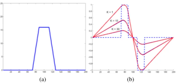
Equation 2 is a diffusion-reaction equation whose analytical solu-tion is not obvious without further assumpsolu-tions on h and g (as de-fined in Sect. 1). For a better understanding, we will analyze the one-dimensional case. We consider edges as ramps which lead to plateau-like patterns in the original gradient (Fig. 2). The equation is decomposed and can be solved onto subdomains {Ωk}0≤k≤Nwhere
gkand hk, the restrictions of g and h to Ωk, are constant. In the
fol-lowing developments, fkwill denote the restriction of a function f
to Ωk.
Two cases arise. If Ωkis a homogeneous region, ∇Ik = 0 so
gk(x) = 1 and hk(x) = 0. Equation 2 is then the one-dimensional
heat equation∂2Vk
∂x2 = 0, so the solution is a linear function:
Vk(x) = mkx + pk, mk, pk∈ R . (3)
If Ωkis a region where the gradient is non-zero, then ∇Ikis
con-stant (due to the ramp model) and so are gkand hk. Equation 2 has
then the form ∂2Vk ∂x2 − a 2 (Vk− ∂I ∂x) = 0 , a 2 = 1 − gk gk , 0 < gk≤ 1 . (4)
Solutions to this second order linear equation with constant coeffi-cients are of the form Vk(x) = c
(1) k e
ax
+ c(2)k e−ax+ b(x), where c(1)k , c(2)k ∈ R and b is a particular solution. Since ∇I is constant over Ωk, it satisfies the equation. Finally, the solutions on such
sub-domains are of the form: Vk(x) = c(1)k e ax + c(2)k e−ax+ ∇I(x) . (5) The parameters mk, pk, c (1) k and c (2)
k for each subdomain Ωk are
given by the Dirichlet boundary condition V = 0 on ∂Ω, the C0and the C1properties of the global solution V at boundaries between the
N subdomains. This yields the following linear system (in the same order): p1 = 0 mNxN+ pN = 0 mk−1xk+ pk−1 = c (1) k e axk+ c(2) k e −axk + v(xk) mk+1xk+1+ pk+1 = ac(1)k e axk+1− ac(2) k e −axk+1 , (6) (a) (b)
Fig. 2: (a) Original signal and (b) the analytical solution of the GVF equation for K = 3, K = 15 and K = 30 (where K is the pa-rameter of function g). The dotted line represents the original nor-malized gradient, the analytical solution is plotted in plain red, and the numeric solution is in plain blue. Both solutions overlap almost completely. The zero-crossings are preserved for all values of K but the positions of the maxima of the solution are clearly impacted.
where xidenotes the point limiting Ωi−1and Ωi, and 0 < k < N .
If there are M plateau-like patterns, this yields a linear system of 4M + 2 equations. A numerical solution and the corresponding ana-lytical solution, computed from a two ramps gradient, are illustrated in Fig. 2. In practice, subdomains Ωkwhere ∇I 6= 0 tend towards
∅, which means that the GVF can be approximated by a piecewise-linear function. Although this is a mere approximation, we will use this property to derive our scale measure.
3. DETECTION OF MEDIAL POINTS AND THEIR CORRESPONDING SCALE
The GVF energy functional in Eq. 1 contains a diffusion term which is equivalent to a multiscale analysis, from a scale-space point of view. The method proposed here is driven by two ideas. First, scale information should be available directly from the GVF, without any further multiscale analysis. Second, since all the work has been done by the GVF, recovering scales should not use overcomplicated anal-ysis schemes of the solution.
In contrast-enhanced images, vascular structures are considered as homogeneous regions surrounded by strong gradients. In those regions, the GVF matches gradients having opposite directions, in some sense. This interpretation still holds in the one-dimensional case: thanks to the separability property of the GVF, one can con-sider working on the projections of the solution V along each dimen-sion instead of working on the gradient vector field itself. It means that analyzing the d-th component Vdof V along the d-th dimension
only is relevant. In this outlook, the separability of the GVF and re-sults from Sect. 2 are exploited both to detect medial points and to estimate the radius of structures.
3.1. Detection of medial points
Matching gradients having opposite directions comes down to matching projections along each dimension d having opposite signs (see Fig. 2). According to Sect. 2, the GVF may be approximated by a linear function and vanishes between those two gradients. To ensure that zero-crossings happen in the center of structures, both corresponding gradients must have exactly the same magnitude. This is why we choose to diffuse the normalized image gradient. In practice, the Point Spread Function (PSF) of the acquisition
sys-regions so that the slope of the solution V is weaker near edges. Along a given dimension d, medial points are thus detected as max-ima ofdVd
dxd, which can still be emphasized by taking the normalized
solution ˜V . Responses are summed over all dimensions to obtain the final measure for medial points:
M = div( ˜V ) =X
d
d ˜Vd
dxd
. (7)
3.2. Estimation of the radius of the structures
Following the remarks formulated in the previous paragraph con-cerning the linear approximation, the slope of Vdis inversely
pro-portional to the radius of the structures. Let rd,kbe the size of the
structures along dimension d, delimited by two matching gradients Vd(xk) and Vd(xk+1) at positions xkand xk+1. The slope mkcan
be recovered where Vdvanishes and the radius can be estimated as:
rd,k=
Vd(xk) − Vd(xk+1)
2mk
. (8)
Knowing the positions xk is not obvious. This is why previous
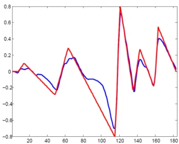
works usually resort to an exhaustive search through multiscale anal-ysis. On the contrary, since we are able to detect structures of inter-est thanks to zero-crossings, we have all the necessary information to approximate Vdwith a piecewise-linear function. We are only
inter-ested in the positions where two linear functions intersect, thus the approximation does not have to be accurate (see Fig. 3). A position xkresponsible for linear regions Ωkand Ωk+1with corresponding
zero-crossings ckand ck+1is thus recovered as:
xk=
mk+1ck+1− mkck
mk+1− mk
. (9)
The actual radius rkcan now be computed with simple geometrical
considerations. For example, for 2D images, the radius is:
rk= r1sin arccos r1 pr2 1+ r22 ! , (10)
where r1and r2are the radii estimated along each direction.
4. EVALUATION OF THE ESTIMATED SCALES AND APPLICATION TO VASCULAR STRUCTURES Equation 2 can be solved with various explicit, implicit or semi-implicit schemes. We implemented the common explicit scheme for simplicity (see Boukerroui, 2009 [8] for more efficient explicit and implicit schemes). In particular, unconditionnally stable explicit schemes exist (the Alternating Direction Explicit scheme, for exam-ple). In practice, the straightforward explicit scheme is still widely used and is very useful for investigation. We recall this scheme (Xu et al., 1998 [3]): Vin+1= (1 − h∆t)V n i + g∆t ∆x (V n
i−1+ Vi+1n − 2Vin) + h∇I∆t ,
(11) where ∆x is the spatial resolution.
Fig. 3: Solution to the GVF (in blue) for a one-dimensional extracted from Fig. 1 and its corresponding piecewise linear reconstruction (in
red).
4.1. Validation on synthetical vessel templates
As mentioned in Sect. 3.1, the PSF of the acquisition system and partial volume effects impact the estimation of the vessels radius. To study their influence, we apply our algorithm to vessel templates with various radii and PSF. Vessels are modeled by convolved bar-like cross-sections with radii r0ranging from 1 to 25 pixels, and the scale of the convolution σP SFis 0.5, 1 and 2 pixels (we approximate
the PSF by a Gaussian distribution).
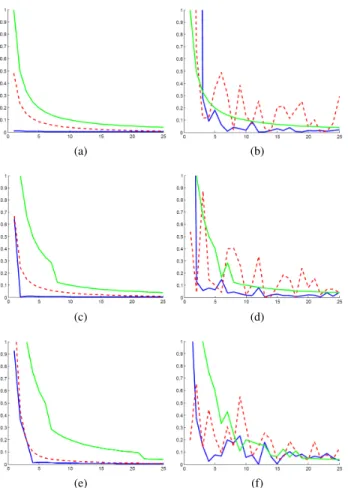
The relative error of the estimation with respect to the ground truth err(r) = |r−rr00| is illustrated in Fig. 4. The algorithm
in-troduced in Sect. 3.2 is represented by blue lines. We compare it with two other approaches. The first one, represented by red lines, is the radius evaluated by taking r = min (|xk− ck|, |xk+1− ck+1|).
The second one, represented by the green lines, correspond to the distance from ckto the closest local maximum of k V k. Finally,
the evaluation was performed on noise-free profiles (K = 5) in the first column, and on profiles with a 10% random additive Gaussian noise (K = 15 to compensate for the presence noise) in the second column.
It is clear that our algorithm performs better for all PSF values and is globally more robust to noise. When r0 ≤ σ
P SF with no
noise, the estimation is clearly unreliable but usable since the error is still less than one pixel. For r0> σP SF, the error is less than 3% for
noise-free profiles, and remains low (around 10%) in the presence of an additive Gaussian noise . However, for radii smaller than the PSF, zero-crossings of the GVF may disappear and thus our algorithm fails to recover the structure, which corresponds to the very high errors in Fig. 4.
4.2. Skeleton extraction of vascular structures
Our algorithm was also tested to extract the skeleton of vascular structures in 2D angiographies. The medialness map M from Eq.7 and the radii are computed from the 2D GVF of the image. Seed points are selected as directional maxima of M and those lying in regions with low local contrast are discarded. Finally, centerlines are extracted as the ridges of M going through seed points. The
(a) (b)
(c) (d)
(e) (f)
Fig. 4: Relative error err of the estimated radius for radii ranging from 1 to 25 pixels and a Gaussian PSF with (a-b) σP SF = 0.5,
(c-d) σP SF = 1, (e-f) σP SF = 2. The first column shows the result
for profiles with no noise, while a 10% random Gaussian noise has been added to vessel templates in the second column (see the text for
further details).
centerlines and a segmentation reconstructed from both types of in-formation are illustrated in Fig. 5. Most vessels are correctly recov-ered, with accurate radii (they are slightly overestimated in the case of very small vessels, as one should expect from Sect. 4.1).
5. CONCLUSION
We presented a new segmentation-free method to extract scale in-formation of vascular structures from the GVF of an image, without any additional multiscale analysis. We demonstrated that, through fast and effective one-dimensional analysis of the GVF, we are able to devise a method which is both accurate and robust to noise. The result can serve as an input for deformable model-based algorithms, to further refine the segmentation. The current bottleneck of our approach lies in the computation of the GVF which is highly time-consuming, as any processes involving diffusion. Efforts will be put on efficient schemes to solve this variational problem. In the future, we believe that our approach will prove to be a good alternative to multiscale analysis.
(a) (b)
(c) (d)
Fig. 5: Two examples of centerlines extracted from the medialness map M and their corresponding vessel segmentation, on 2D X-ray
angiographies.
6. REFERENCES
[1] Xu, C. and Prince, J.L., “Snakes, Shapes, and Gradient Vector Flow,” IEEE Transactions on Image Processing, vol. 7, no. 3, pp. 359–369, 1998.
[2] Xu, C. and Prince, J.L., “Global Optimality of Gradient Vector Flow,” Proc. of 34th Annual Conference on Information Sci-ences and Systems, pp. 1–2, 2000.
[3] Xu, C. and Prince, J.L., “Generalized Gradient Vector Flow External Forces for Active Contours,” Signal Processing, vol. 71, pp. 131–139, 1999.
[4] Bauer, C., Bischof, H. and Beichel, R., “Segmentation of Air-ways Based on Gradient Vector Flow,” International Workshop on Pulmonary Image Analysis (Medical Image Computing and Computer Assisted Intervention), pp. 191–201, 2009.
[5] Engel, D. and Curio, C., “Scale-invariant Medial Features Based on Gradient Vector Flow Fields,” Proc. of 19th International Conference on Pattern Recognition, pp. 1–4, 2008.
[6] Yu, Z. and Bajaj, C., “A Segmentation-Free Approach for Skele-tonization of Gray-Scale Images via Anisotropic Vector Diffu-sion,” Computer Vision and Pattern Recognition, vol. 1, pp. 415–420, 2004.
[7] Hassouna, M.S. and Farag, A.A., “On the Extraction of Curve Skeletons using Gradient Vector Flow,” Proc. of 11th Interna-tional Conference on Computer Vision, pp. 1–8, 2007.
[8] Boukerroui, D., “Efficient Numerical Schemes for Gradient Vector Flow,” Proc. of 16th International Conference on Im-age Processing, pp. 4057–4060, 2009.