HAL Id: tel-01735320
https://pastel.archives-ouvertes.fr/tel-01735320
Submitted on 15 Mar 2018HAL is a multi-disciplinary open access
archive for the deposit and dissemination of sci-entific research documents, whether they are pub-lished or not. The documents may come from teaching and research institutions in France or abroad, or from public or private research centers.
L’archive ouverte pluridisciplinaire HAL, est destinée au dépôt et à la diffusion de documents scientifiques de niveau recherche, publiés ou non, émanant des établissements d’enseignement et de recherche français ou étrangers, des laboratoires publics ou privés.
Model Averaging in Large Scale Learning
Edwin Grappin
To cite this version:
Edwin Grappin. Model Averaging in Large Scale Learning. Statistics [math.ST]. Université Paris-Saclay, 2018. English. �NNT : 2018SACLG001�. �tel-01735320�
NNT : 2018SACLG001
Thèse de doctorat
de l’Université Paris-Saclay
École doctorale de mathématiques Hadamard (EDMH, ED 574)
Etablissement d’inscription : ENSAE ParisTech
Etablissement d’accueil : CREST (UMR CNRS 9194) - Laboratoire de Statistiques
Spécialité de doctorat : Mathématiques fondamentales
Edwin Grappin
Estimateur par agrégat en apprentissage statistique
en grande dimension
Soutenue le 6 mars 2018 à l’ENSAE ParisTech, Palaiseau.
Après avis des rapporteurs : Jalal Fadili (GREYC CNRS, ENSICAEN) Karim Lounici (Georgia Institute of Technology)
Jury de soutenance : Cristina Butucea (Université Paris-Est) Examinateur Ismaël Castillo (Université Sorbonne) Examinateur Arnak Dalalyan (CREST - ENSAE - GENES) Directeur de thèse Jalal Fadili (GREYC CNRS, ENSICAEN) Rapporteur
Mohamed Hebiri (Université Paris-Est) Examinateur Alexandre Tsybakov (CREST - ENSAE - GENES) Président de jury
NNT : 2018SACLG001
Thesis presented for the title of Doctor of Philosophy
at Université Paris-Saclay.
Doctoral School of Mathematics Hadamard (EDMH, ED 574)
University : ENSAE ParisTech
Hosting research center: CREST (UMR CNRS 9194) - Laboratoire de Statistiques
Doctoral specialty: Fundamental mathematics
Edwin Grappin
Model Averaging in Large Scale Learning
6th March 2018 at ENSAE ParisTech, Palaiseau.
Reviewing committee : Jalal Fadili (GREYC CNRS, ENSICAEN) Karim Lounici (Georgia Institute of Technology)
Ph.D. committee : Cristina Butucea (Université Paris-Est) Ismaël Castillo (Université Sorbonne)
Arnak Dalalyan (CREST - ENSAE - GENES) - Ph.D. Supervisor Jalal Fadili (GREYC CNRS, ENSICAEN)
Mohamed Hebiri (Université Paris-Est)
Model Averaging in Large Scale Learning
Edwin Grappin
Submitted for the degree of Doctor of Philosophy at Université Paris-Saclay
February 2018
Abstract
This thesis explores both statistical and computational properties of estimations procedures closely related to aggregation in the problem of high-dimensional regression in a sparse setting. The exponentially weighted aggregate is well studied in the machine learning and statistical literature. It benefits from strong results in fixed and random design with a PAC-Bayesian approach. However, little is known about the properties of the exponentially weighted aggregate with Laplace prior. In Chapter2we study the statistical behaviour of the prediction loss of the exponentially weighted aggregate with Laplace prior in the fixed design setting. We establish sharp oracle inequalities which generalize the properties of the Lasso to a larger family of estimators. These results also bridge the gap from the Lasso to the Bayesian Lasso as these estimators belong to the class of estimators we consider. Moreover, the method of the proof can be easily applied to other estimators. Oracle inequalities are proven for the matrix regression setting with the nuclear norm prior. In Chapter 3 we introduce an adjusted Langevin Monte Carlo sampling method that approximates the exponentially weighted aggregate with Laplace prior in an explicit finite number of iterations for any targeted accuracy. These works generalize the results proved in Dalalyan (2017) in order to apply theoretical guarantees for non-smooth priors such as the Laplace prior. In Chapter 4, we study a complementary subject, namely the statisctical behaviour of adjusted versions of the Lasso for the transductive and semi-supervised learning task in the random design setting. Upperbound on the prediction risk, in both deviation and expectation, are proved and we point out that unlabeled features can substantially improve bounds on the prediction loss.
Estimateur par agrégat en apprentissage statistique en
grande dimension
Edwin Grappin
Thèse présentée dans le cadre d’un doctorat à l’Université Paris-Saclay
Février 2018
Abstract
Les travaux de cette thèse explorent les propriétés statistiques et computationnelles de procé-dures d’estimation par agrégation appliquées aux problèmes de régression en grande dimension dans un context parcimonieux (ou sparse). Les estimateurs par agrégation à poids exponen-tiels font l’objet d’une abondante littérature dans les communautés de la statistique et de l’apprentissage automatisé. Ces méthodes bénéficient de résultats théoriques optimaux sous une approche PAC-Bayésienne dans le cadre de données aléatoires ou fixes. Cependant, le com-portement théorique de l’agrégat avec prior de Laplace n’est guère connu. Ce dernier représente pourtant un intérêt important puisqu’il est l’analogue du Lasso dans le cadre pseudo-bayésien. Le Chapitre 2explicite une borne du risque de prédiction de cet estimateur, généralisant ainsi les résultats du Lasso. De ce fait, nous montrons aussi que pour certains niveaux faibles de la température, l’estimateur bénéficie de bornes optimales. Le Chapitre3prouve qu’une méthode de simulation s’appuyant sur un processus de Langevin Monte Carlo permet de choisir expli-citement le nombre d’itérations nécessaire pour garantir une qualité d’approximation souhaitée. Le Chapitre 4 introduit des variantes du Lasso pour améliorer les performances de prédiction dans des contextes partiellement labélisés.
Declaration
The work in this thesis is based on research carried out at ENSAE with the Statistics department of CREST, France.
This work is licensed under the Creative Commons Attribution 4.0 International License. To view a copy of this license, visit https://creativecommons.org/licenses/by-sa/4.0/.
Dedicated to
Bérengère, Pierre and my parents without whom this thesis would have never been possible. Had they not pretended to find interesting what I was doing for such a long time, this journey
Acknowledgements
First and foremost I want to thank Arnak, my Ph.D. advisor. Not only Arnak is one of the most passionate and pedagogic professors I have ever met, he also proves himself to be an understanding, supportive and benevolent advisor. Arnak introduced me to incredibly stimulating statistical questions and I appreciate all his contributions of support, time and ideas to make my Ph.D. experience the best it could have been. His guidance was invaluable and I could not imagine having a better advisor and mentor for my Ph.D journey.
I am also very grateful to the examiners of this thesis, namely Karim Lounici and Jalal Fadili for their time and their kind feedbacks on this work. And I want to thank the members of my dissertation committee: Cristina Butucea, Alexandre Tsybakov, Jalal Fadili, Mohamed Hebiri, Ismaël Castillo, and Arnak Dalalyan.
The members of the Statistical laboratory have substantially contributed to my personal and professional time at CREST. They have all been very supportive and have provided me with numerous advice and some very thoughtful insights. This laboratory is a great place to both explore Statistics and enjoy a tremendous environment. Obviously, I am grateful to Alexandre Tsybakov, who manages and has gathered so many talented and enthusiastic professors in the Statistics laboratory. I am also grateful for the excellent example he has provided as a great Statistician and professor.
Among all the members of the laboratory, I have a special thought for Pierre Alquier who brings life to the coffee room (and the working groups) and who always has had a spare dose of coffee when the most needed. I think Pierre has helped every Ph.D. student I know from the Statistics laboratory to make our thesis as enjoyable as possible. On a personal note, I consider Pierre as a friend. He has always been there during both the difficult times as well as the most exciting periods of this three-year journey. Looking backward, I doubt my Ph.D. would have been possible without Pierre. I am also very grateful to Nicolas Chopin, Judith Rousseau, Cristina Butucea, Marco Cuturi, Nicolas Chopin, Massimiliano Pontil, Anna Simoni, Olivier Catoni and Guillaume Lecué who have offered their points of view and their knowledge with a
tremendous enthusiasm.
It goes without saying that I am thankful to all the Ph.D. students of the laboratory. I could only start with James, with whom I shared the same office for two years and who taught me the do’s and dont’s of the Ph.D. student life. I am grateful to Alexander, the Ph.D. successor of James (they were both under the supervision of Nicolas Chopin) for his enthusiasm and all the great time we spent together. I am grateful to Mehdi for the incredible human being he is and all the support he brings me at some important times. All the PhD students I had the chance to meet during my Ph.D. study brought this very contagious enthusiasm that I dearly appreciate: Pierre Bellec, Mohamed, The Tien, Léna, Gautier, Lionel, Philippe and Vincent. I gratefully acknowledge the financial fundings that made my Ph.D. possible. I have been funded by the Labex Ecodec and the CREST. I am glad I had the opportunity to study within the Ph.D. program in Mathematics “Ecole Doctorale de Mathématiques Hadamard” (EDMH) of the Université Paris-Saclay.
Lastly, I would like to thank my family and my friends for all their love and encouragement. My Ph.D. time was made enjoyable thanks to my dearest friends Rudy, Arthur, Alexis, Guil-laume Moby and Nicolas who have all been very supportive and have shared some great and unforgetable moments with me. I want to thank Pierre for his incredible support and all the things we have lived together the last three years. Pierre is a very unique person that has proven his loyalty and his determination by helping me through my Ph.D. journey. The last 10 years, I had the chance to be part of the Ultimate Frisbee community and I am grateful to my teammates and all the players, coaches, mentors who I crossed onto fields around the world and are inspiring examples of the values I cherish the most.
Obviously, I am thankful to my parents who raised me with a love for science and supported me in all my pursuits, whatever they are. Last but not the least, I would like to thank Bérengère for her loving support and her incredible patience she showed during this long journey. Thank you.
Edwin Grappin March 2018
Estimateur par agrégat en apprentissage statistique en
grande dimension
Résumé Substantiel
Soient 𝑛 et 𝑝 des entiers strictement positifs. Considérons le couple (𝑋, 𝑦) ∈ (R𝑛×𝑝× R𝑛) tiré
d’une distribution 𝑃 sur l’espace 𝒳 × 𝒴. Dans le cadre d’un problème de régression, l’objectif est de prédire le vecteur 𝑦 à partir d’un jeu de données 𝑋. Une approche possible consiste à estimer une fonction 𝑓 : 𝒳 → 𝒴 qui minimise le risque
ℛ(𝑓 ) = ∫︁
𝒳 ×𝒴
𝑙(𝑦, 𝑓 (𝑥)) 𝑃 (d𝑥, dy), (0.0.1)
où 𝑙 est une fonction de perte arbitrairement choisie. Nous appelons 𝑓⋆ la fonction qui minimise
Equation 0.0.1. Dans ce cas, le problème de régression peut s’écrire sous la forme
𝑦 = 𝑓⋆(𝑋) + 𝜉, où 𝜉 ∈ R𝑝 est un vecteur de variables aléatoires.
Etude théorique de l’EWA avec
prior de Laplace
L’apport principal de ce manuscrit est l’étude du comportement théorique de l’estimateur par agrégation avec prior de Laplace lorsqu’il existe une représentation quasi-parcimonieuse1 de la
relation fonctionnelle qui lie 𝑦 au jeu de données X.
L’estimation par agrégation à poids exponentiels est une méthode efficace pour inférer un signal dans un cadre quasi-parcimonieux (Dalalyan and Tsybakov,2012a,b). Différents priors ont été étudiés dans la litérature de l’apprentissage statistique. Il est intéressant de remarquer que le prior de Laplace n’a jamais été utilisé efficacement.
L’estimateur par agrégat avec prior de Laplace représente un intérêt théorique puisqu’il est l’analogue pseudo-bayésien de l’estimateur Lasso. L’estimateur Lasso est certainement l’estimateur le plus largement étudié (et utilisé) parmi les méthodes de régression pénalisée dans un con-texte quasi-parcimonieux en grande dimension. En dépit de ses avantages computationnels et
1Le lecteur est invité à lire la suite de ce manuscrit pour obtenir une compréhension plus complète de la
théoriques, les garanties d’inégalités oracle optimales pour le Lasso nécessitent des hypothèses restrictives sur le jeu de données X.
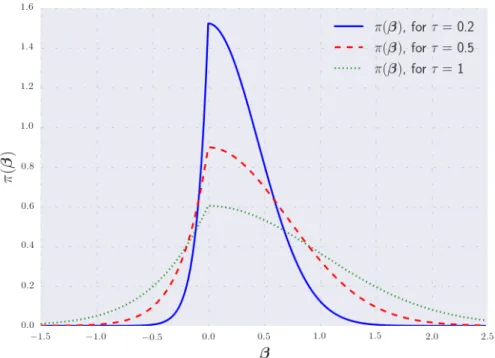
A contrario, les estimateurs par aggrégation à poids exponentiels (EWA) bénéficient de résultats théoriques optimaux sous une approche PAC-Bayésienne dans le cadre de données aléatoires ou fixes avec des hypothèses moins contraignantes. A ce jour, l’EWA avec prior de Laplace est peu étudié. Le Chapitre 2 explicite une borne du risque de prédiction de cet estimateur, généralisant ainsi les résultats du Lasso. De ce fait, nous montrons aussi que pour de faibles niveaux du paramètre de température, l’estimateur bénéficie de bornes optimales.
Le principal objet d’étude de cette thèse est la régression linéaire où l’on cherche à prédire 𝑦 par une relation linéaire entre le jeu de données X et un vecteur 𝛽 ∈ R𝑝
𝑦 = X𝛽 + 𝜉, (0.0.2)
où l’on cherche à estimer 𝛽 de sorte à minimiser une fonction de perte.
Dans ce contexte, le Théorème 2.3.1 du Chapitre2 est une version simplifiée des résultats. Il permet de mettre en évidence l’impact du choix du paramètre de température 𝜏 sur la borne du risque de prédiction.
Le Théorème 2.4.1 explicite des résultats de type concentration du pseudo-posterior. Ces ré-sultats sont généralisable à d’autres prior et à d’autres contextes tels que la régression matri-cielle. Ainsi les Théorèmes 2.5.1 et2.5.2 du Chapitre 2étendent ces résultats au cas matriciel.
Etude théorique d’une méthode de simulation de l’EWA
avec
prior de Laplace
Si le Chapitre 2 permet de regrouper les résultats théoriques du Lasso et de son analogue pseudo-bayésien, le Chapitre 3 en étudie l’aspect computationnel. Garantir l’existence d’une méthode qui approche efficacement cet estimateur s’avère être un défi plus difficile. Cela reste cependant essentiel pour que l’EWA avec prior de Laplace soit utilisable en pratique. En nous appuyant sur les travaux deDalalyan (2016),Durmus and Moulines (2016) etDalalyan (2017) nous étudions le comportement d’une méthode de simulation par Langevin Monte Carlo pour approcher cet estimateur.
Une application directe d’un processus de Langevin Monte Carlo comme présenté dans (Dalalyan,
2016, 2017; Durmus and Moulines, 2016) ne garantirait pas nécessairement l’obtention d’une précision souhaitée après un nombre fini d’itérations. En effet, ces résultats nécessitent que le
posterior soit fortement convexe et lisse alors que dans le cas du prior de Laplace le log-posterior n’est pas différentiable. De même, la forte convexité n’est pas respectée pour tout jeu de données. Dans le Chapitre 3, nous résolvons partiellement cette question. Nous étudions le comportement d’une simulation de la discrétisation d’Euler d’un processus de Langevin Monte Carlo. Plus particulièrement, nous étudions la qualité de la simulation au sens de la distance de Wasserstein par rapport à l’agrégat à poids exponentiels avec prior de Laplace ciblé. L’approche consiste à adapter le travail de Dalalyan (2016) afin de contourner la non différentiabilité du pseudo posterior. Nous explicitons un nombre d’itérations 𝐾 du même ordre de grandeur que le nombre d’itérations nécessaires dans Dalalyan (2016) en vue d’une tolérance à l’erreur 𝜖 et de la dimension 𝑝. Il s’agit de noter que cette ébauche de résultat ne résout pas entièrement la question computationnelle. En effet, ces résultats sont garantis sous l’hypothèse de forte convexité. Cela requiert notamment des hypothèses trop restrictives sur la matrice de Gram. En particulier, ces hypothèses ne sont pas réalistes dans un problème en grande dimension. En effet, dans le Chapitre3, nous supposons que la plus petite valeur propre de la matrice de Gram est strictement positive. Malgrés ces limites cette étude définie une méthode computationnelle qui garantie une approximation précise d’une densité ciblée dans une situation légérement plus généralisée que la littérature existante.
Apprentissage transductif et semi-supervisé
Le Chapitre 4est une étude de l’estimateur Lasso dans des contextes semi-supervisés ou trans-ductifs. Il peut être lu indépendemment du reste de ce manuscrit bien qu’il complète et peut se voir complété par les résultats des autres chapitres de cette thèse. Nous montrons que des données non labélisées devraient être utilisées dans le calcul de l’estimateur afin d’inférer la matrice de variance-covariance. Ainsi, nous présentons deux adaptations de l’estimateur Lasso afin d’améliorer les performances de prédiction dans un cadre d’apprentissage transductif ou partiellement labélisé. Sous certaines hypothèses, nous démontrons des inégalités oracle opti-males dans le cadre de designs aléatoires.
Contents
Cover page - French i
Cover page ii Abstract iii Abstract - French iv Declaration v Acknowledgements vii French Summary ix 1 Introduction 1 1.1 Context . . . 2
1.1.1 The rise of Statistics . . . 2
1.1.2 Definition of Statistics . . . 5
1.1.3 Examples of applications . . . 7
1.1.4 Supervised, unsupervised and partially labeled learning . . . 10
1.2 Challenges in high-dimensional statistics . . . 11
1.2.1 High-dimensional statistics . . . 11
1.2.2 Sparsity . . . 14
1.2.3 Prediction risk and oracle inequality . . . 17
1.2.4 Oracle inequality in the sparsity context . . . 19
1.3 Maximum a posteriori estimation . . . 21
1.3.1 Penalized regression and MAP . . . 21
1.3.2 The Lasso estimator and related estimators . . . 23
1.4 The PAC-Bayesian settings and aggregation estimators . . . 26
1.4.1 The concept of PAC-learning . . . 27
1.4.2 Literature in the PAC-Bayesian community . . . 29
1.4.3 Aggregation . . . 31
1.4.4 Exponentially weighted aggregation and its variations . . . 34
1.4.5 Computational challenges and Langevin Monte Carlo . . . 37
1.5 Roadmap . . . 40
2 On the Exponentially Weighted Aggregate with the Laplace Prior 43 2.1 Introduction . . . 44
2.2 Notation . . . 49
2.3 Risk bound for the EWA with the Laplace prior . . . 50
2.4 Pseudo-Posterior concentration . . . 53
2.5 Sparsity oracle inequality in the matrix case . . . 56
2.5.1 Specific notation . . . 56
2.5.2 Nuclear-norm prior and the exponential weights . . . 57
2.5.3 Oracle Inequality . . . 58
2.5.4 Pseudo-posterior concentration . . . 60
2.6 Conclusions . . . 61
2.7 Proofs . . . 62
2.7.1 Proof of the oracle inequality of Theorem 2.3.1. . . 62
2.7.2 Proof of the concentration property of Theorem 2.4.1 . . . 64
2.7.3 Proof of Proposition 2.3.1 . . . 65
2.7.4 Proofs for Stein’s unbiased risk estimate (2.3.7) . . . 67
2.7.5 Proof of the results in the matrix case . . . 69
3 Computation guarantees with Langevin Monte Carlo 77 3.1 Introduction, context and notations . . . 78
3.1.1 Notations . . . 80
3.1.2 The Langevin Monte Carlo algorithm . . . 82
3.2 Guarantees for the Wasserstein distance of subdifferentiable potentials . . . 83
3.2.1 Theoretical guarantees from Durmus and Moulines (2016) and Dalalyan (2017) . . . 84
3.2.2 Bounding the Wasserstein distance between approximation and the target
distribution . . . 87
3.2.3 Conclusion on theoretical guarantees in finite sampling . . . 90
3.3 The case of EWA with Laplace prior approximation . . . 91
3.4 Discussion and outlook . . . 99
3.5 Proofs . . . 100
3.5.1 Proof of Proposition 3.3.1 . . . 100
3.5.2 Proof of Proposition 3.3.2 . . . 104
3.5.3 Proof of Corollary 3.3.2 and Remark 3.3.1 . . . 105
4 On the prediction loss of the lasso in the partially labeled setting 113 4.1 Introduction . . . 114
4.2 Notations . . . 119
4.3 Brief overview of related work . . . 120
4.4 Risk bounds in transductive setting . . . 124
4.5 Risk bounds in semi-supervised setting . . . 126
4.6 Conclusion . . . 130
4.7 Proofs . . . 131
4.7.1 Proof of 4.4.1 . . . 134
4.7.2 Proofs for the semi-supervised version of the lasso . . . 135
4.7.3 Bernstein inequality . . . 142
List of Figures
1-1 A hard drive in 1956 . . . 4
1-2 The risk of spurious correlation . . . 10
1-3 Underfitting and overfitting risks representations . . . 13
1-4 Image representations of faces . . . 14
1-5 Face averaging for image classification. . . 15
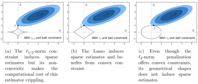
1-6 The geometry of penalizations . . . 25
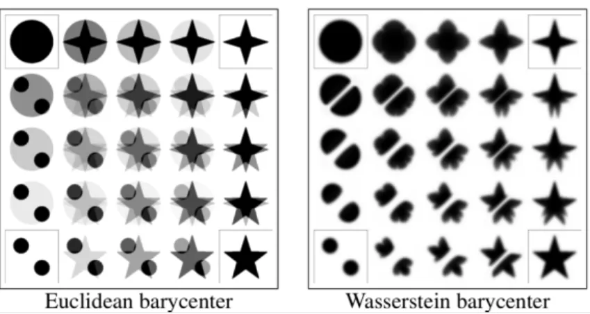
1-7 Euclidean versus Wasserstein barycenter in shape interpolation . . . 39
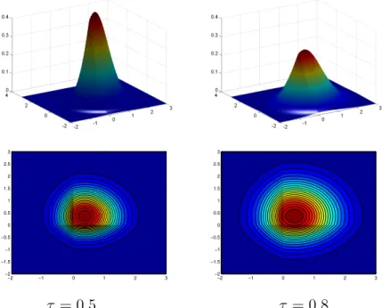
2-1 The impact of the temperature on pseudo-posterior measure . . . 46
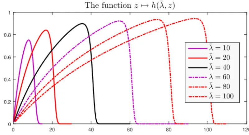
2-2 On the term 𝐻(𝜏) and the tightness of the EWA oracle inequality . . . 52
3-1 The impact of the temperature on the potential . . . 93
3-2 The smooth approximation of the ℓ1 penalization . . . 94
Chapter 1
Introduction
Contents
1.1 Context . . . 2
1.1.1 The rise of Statistics . . . 2
1.1.2 Definition of Statistics . . . 5
1.1.3 Examples of applications. . . 7
1.1.4 Supervised, unsupervised and partially labeled learning . . . 10
1.2 Challenges in high-dimensional statistics . . . 11
1.2.1 High-dimensional statistics . . . 11
1.2.2 Sparsity . . . 14
1.2.3 Prediction risk and oracle inequality . . . 17
1.2.4 Oracle inequality in the sparsity context . . . 19
1.3 Maximum a posteriori estimation . . . 21
1.3.1 Penalized regression and MAP . . . 21
1.3.2 The Lasso estimator and related estimators . . . 23
1.3.3 Review of literature . . . 25
1.4 The PAC-Bayesian settings and aggregation estimators . . . 26
1.4.1 The concept of PAC-learning . . . 27
1.4.2 Literature in the PAC-Bayesian community . . . 29
1.4.3 Aggregation . . . 31
1.4.4 Exponentially weighted aggregation and its variations . . . 34
1.5 Roadmap . . . 40
1.1
Context
1.1.1
The rise of Statistics
Over the last decades, Statistics has been at the center of attention, in a wide variety of ways. Hardly a day goes by without one hearing about Statistics, Artificial Intelligence, Machine Learning or Big Data. Large companies such as Google, Apple, Facebook and Amazon (also known as GAFA) or Baidu, Alibaba, Tencent and Xiaomi (sometimes called BATX) play an important role in the mainstream status of all these technical terms. What can be done with data and the computer resources that are recently accessible causes a lot of ink to flow and is subject to a great deal of thoughts and speculations. While some consider artificial intelligence as a threat for the future of humanity1, others see their applications for the greater good, and
are very optimistic about the impact of artificial intelligence applications, such as automated or assisted medical diagnoses for early detection, or robots that substitute for humans in laborious chores. If the impact of artificial intelligence on the future is not well understood, it seems to be a great consensus that its applications are going to be a key changer of the day-to-day life. Recent improvements, such as the first weak artificial intelligence algorithm, AlphaGo, that can outperform the best Go masters in the world, have reinforced the common belief that artificial intelligence is intended to a bright future. As discussed in McCarthy and Hayes (1969), with such unclear questions at stakes, it is clear that philosophical and ethical guidelines are to be questioned and that national and international regulations will be necessary to ensure a positive impact of artificial intelligence applications.
The rise of challenges and breakthroughs put under the name of artificial intelligence has been made possible with technological improvements. The most important being the increase of computer performance and the soar of sharing data capacity with the Internet democratization. As pointed out by Chen(2016), the number of possible floating-point operations per second in CPU and GPU has dramatically increased over the last ten years (see Chen (2016)[Figure 4]). The Moore’s law, introduced for the first time in 1975Moore(1975), predicted that the number of components for each chip would double every single year. This early prediction has been proven to be true until now. From 1991 to 2011, the microprocessors performance has grown
1For example, the open letter Hawking et al.(2015) has been signed by researchers in artificial intelligence
and robotics as well as other non-scientist notorieties, such as Elon Musk, CEO of SpaceX and Tesla Inc., who stated that artificial intelligence is one of today’s ”biggest existential threats” (Crawford(2016);Markoff(2015)).
1000-fold. This dramatic increase mentioned in Borkar and Chien (2011) is supposed to face new challenges. The energy is becoming the limit and will curb the increase of microprocessor frequency. As a result, large-scale parallelism is one of the promising paths to push the increase of performance. Storage capacity has dramatically increased while the price of storage has curbed. This is why it is possible to store more and more data. And with the increase of computer performance, this large amount of data can be processed at large scale2. The last
needed improvement was the ability to share data and computer resources. With the Internet speed increase, this has been made possible.
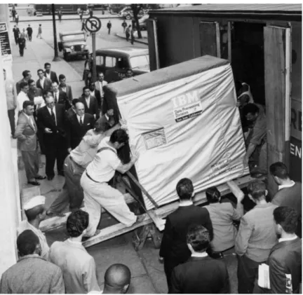
On the one hand, it is now very easy to send large amounts of data through the Internet. Data can be more easily shared, mutualised and used. One agent can produce data while another agent can process or use the data. For example, a dramatic comparison that can be made is the first hard drive disk commercialized by IBM in 1956 (the RAMAC 350) and the last serie of hard drive built by IBM in 2002 (the star serie) (Wikipedia (2017)). While the RAMAC 350 had a storage capacity of 5 Megabytes, its actual volume was approximately two cubic meters; it required a power of 625 watt per Megabyte and its cost was $9, 200 per Megabyte. To get an idea of how big the hardware was at that time, Figure 1-1 shows the transportation of a RAMAC 350 in 1956. On the other hand, the Travelstar 80GN had a 80-Gigabyte capacity, it only requires a power of 0.02 watt per Megabytes and would only cost $0.0053 per Megabyte3.
Additionally, the fact that data can be relatively easily shared implies that computing resources can be outsourced and used when needed. Cloud computing solutions offer on demand com-puting resources. This has only been made possible by the ease of sending data over the net. By facilitating the capacity of producing, sharing, storing and processing data, the aforemen-tioned technological improvements reshape our economical environment. Data, and information extracted from it, become very valuable and strategical assets in our economy. Some compan-ies, such as Alphabet (Google’s parent company), offer free services in order to gather user data. Smartphones and the very common use of the Internet produce considerable amounts of personal data. These data are valuable for many purposes, such as getting insights on social trends, improving marketing strategies by using customer data, or even training and reinfor-cing predictive artificial intelligence algorithms which require important amounts of data to be trained. As data become valuable assets with very strong potential due to computer perform-ance and artificial intelligence progress, it is clear that institutions are urged to regulate the use of data and define some ethics guidelines.
2Of course, the complexity of computational algorithms to process data is a key limit in the capacity of
current processes. It will be one of the topics we will take into consideration in this thesis.
Figure 1-1: A 5-Megabyte IBM hard drive transported in 1956. Photo credit: IBM Company.
If everyone talks about artificial intelligence, we should be aware that the biggest breakthroughs in artificial intelligence are algorithms based on statistical methods with great computing im-plementations. The algorithm AlphaGo, described inSilver et al.(2016), has been developed by Google and uses tree search and neural networks. Autonomous car innovations mainly rely on image recognition, object detection and trajectory decision. The state of the art algorithms to achieve these operations use Machine Learning algorithms such as support vector machine, as in
Levinson et al.(2011), and/or neural networks, as inPomerleau(1991). Machine and statistical learning are subareas of artificial intelligence. Arguably, not every method used in artificial in-telligence comes from Statistics or Machine Learning. For example, the study Olmstadt(2000) describes the early expert systems only which used human knowledge, in which there were no learning steps in the process. However, the most intricate decisions and challenging operations are based on learning new representations of the environment and detecting patterns in order to take decisions, which are tasks achieved by statistical methods. This is the goal of Machine Learning methods, that we will not differentiate from statistical learning in this thesis. In order to provide the reader with a better understanding of what is Statistics and of the context of this thesis, we will define some concepts that will be used throughout this thesis.
1.1.2
Definition of Statistics
According to Donoho (2015), the term and the use of Statistics were introduced 200 years ago along with the need to collect census data about the inhabitants of a given country. The statistical tools have been limited for a long time by the size of the data and the capacity to store and process the information, no computer being available. The introduction of the first automated systems, such as punch card tabulators, was the beginning of the capacity of scaling the amount of data that could be stored and eventually processed. From this point of view, Statistics is a boundless field that could be summarized in a very large sense as the definition of Statistics given by Agresti and Finlay(1997).
Definition 1.1.1 (Statistics). Statistics consists of a body of methods for collecting and ana-lyzing data.
Defined as such, some questions have been treated by statisticians over time, from both theor-etical and empirical points of view. With no claim of being exhaustive, we can mention:
Data collection and storage This subarea tackles some questions such as the type of data that should be collected, and the way the data should be stored, referenced and organized. Polling has been a very deeply studied subject, asking some questions such as how many observations we need or how we can collect a survey with a small bias. On a larger extent, some questions about compressing data to limit storage costs, while loosing as little as possible information can be seen as part of this area.
Inference Statistical inference is a set of data analysis methods that help interpreting empir-ical observations. The purpose of estimation is often to understand a phenomenon by evaluating parameters that could explain the behaviour of a studied sample, or even a larger set that is supposed to be well represented by this given sample. The term of causal inference is used when the goal is to explain the causal interactions in a given model. The bookPearl et al.(2016) provides an excellent explanation of the difference between simple association and causal relationships in Statistics.
Prediction According to Shmueli(2010), predictive modeling is the process of applying stat-istical methods in order to predict the observation of a new individual. We will go into further details later in this section. FromDonoho (2015), statistical prediction is defined as predicting what responses are going to be for future inputs.
Quality assessment The question of measuring the quality of statistical methods has been of paramount concern throughout the history of Statistics. How accurate is a prediction? How representative is a modeling inference to the real observations? Such questions are at the core of the statistical theory discipline.
This list, far from being exhaustive, comes under a plethoric literature. These different fields of study have very strongly developed from some simple results to very complex and subtle results. Some estimation methods have been thoroughly studied and the literature guarantees that the quality of these estimations are well understood in a given context.
If such a definition of Statistics is very large, it seems to conflict with other disciplines such as Machine Learning. In the following section, we will point out some similarities and differences between Statistics and Machine Learning. As it is not the topic of this thesis, we discuss it very briefly. For any reader who wishes a deeper understanding of the definition of these fields, we could only recommend the papers Donoho (2015), Breiman (2001), and the book Wasserman
(2013), that are great food for thoughts on these matters.
Machine learning is very similar to Statistics. In view of Definition 1.1.1, both are studying methods to collect and analyze data. Since Statistics is a much older discipline than the inven-tion of computers, statisticians could claim that Machine Learning is a mere clone of Statistics. However, the origins of Machine Learning differ from those of Statistics. This is why these two communities have distinct terms and sometimes different purposes. According to Wasser-man (2013), Machine Learning comes from computer science departments. In Wasserman
(2013)[Preface], a table of vocabulary equivalence between Machine Learning and Statistics is presented. It is worth remarking that there is a trend in both fields to share more and more terms. As an example, the term learning arised from Machine Learning is now very commonly used in the area of statistical learning. Originally, as statisticians did not have access to the calculus capacities of computers, low-dimensional problems were considered. Moreover, as poin-ted out in Breiman (2001), the issue of inference was initially prioritized over the question of prediction. This is explained by a long tradition of Statistics as being the inference from a data sample of an unknown underlying generative models. On the contrary, the Machine Learning community often worked without probability assumptions on the model; consequently, the field has been mainly focused on the prediction issue and, of course, computational challenges. As a consequence, there are differences between Machine Learning and Statistics. However, as there exist communities within Statistics and Machine Learning, it seems fair to admit that these two disciplines are also two communities working on same challenges with different backgrounds.
The focus and vocabulary of these disciplines tend to converge over time.
1.1.3
Examples of applications
There is a tremendous amount of current and potential applications of Statistics in our environ-ment. While some of these applications are very well-known, some others are used in our daily life without us being aware of it. Earlier, we mentioned Google AlphaGo (Silver et al.(2016)), the first algorithm which managed to outperform any living human at playing the board game Go. The paperBouzy and Cazenave (2001) provides an analysis of Go from a statistical point of view. Other games are being, or have been, learned by algorithms and are strongly advert-ized. Of course, our first thought goes to the famous IBM Deep Blue algorithm that defeated the best chess players in the world, as explained in Campbell et al. (2002) and Sutton and Barto (1998). The book Hsu (2002) provides interesting insights on Deep Blue story. It is worth noting that building a world-class algorithm playing Go has been more challenging than developing a Chess computer. The main reason of this difficulty gap is mainly the much higher number of possible combinations in Go, as explained in Burmeister and Wiles (1995).
Other applications are of paramount importance in our society. The healthcare industry has strongly benefited from statistical algorithms. The diagnosis of various diseases can be auto-mated or assisted. The review in Kononenko (2001) mentions several statistical methods such as naive and semi-naive Bayesian classifiers, k-nearest neighbors, neural networks or decision trees. The article Dreiseitl et al. (2001) compares algorithms such as logistic regression, arti-ficial neural networks, decision trees, and support vector machines on the task of diagnosing pigmented skin lesions, in order to distinguish common nevi from dysplastic nevi or melanoma. The authors of Shipp et al.(2002) describe a method to ease the detection of blood cancer. The discovery of new drugs in the pharmaceutical industry is a growing challenge. The more active compounds are discovered, the less likely it is to discover a new drug with positive impact. In order to keep innovating, the pharmaceutical industry needs to increase the capacity of screening active compounds. Standard high-throughput screening methods become more and more costly as the number of active compounds already tested increases. As in ranking
Agarwal et al.(2010), Machine Learning solutions enable to screen million of active compounds to rank them according to their likelihood to match a given response target. Statisticians and computer scientists developed digital high-throughput screening solutions based on support vector machine methodsBurbidge et al.(2001) and neural networksByvatov et al.(2003). The domain of active learning (Warmuth et al., 2003) plays an important role in the early phases
of drug discovery.
Image analysis plays a central role in radiology and medical imaging. Numerous examples are developed in the literature. Methods to detect microcalcifications from mammograms are compared in Wei et al. (2005). These methods include support vector machine, kernel Fisher discriminant and ensemble averaging. A review of various radiology applications is made in
Wang and Summers (2012). Image segmentation, computer-aided diagnosis, neurological dia-gnosis are among the most astonishing applications of Machine Learning. Artificial intelligence can support the field of medicine with many other applications, such as health monitoring devices that can analyze data from patients (Bacci, 2017; Boukhebouze et al., 2016; Graham,
2014;Roux et al.,2017). On a larger scale, the detection of epidemiological outbreaks (Aramaki et al., 2011; Culotta, 2010) can be done with Bayesian network modeling, as in Wong et al.
(2003), or with support vector machine and logistic classification as inAdar and Adamic(2005). As mentioned earlier, the field of autonomous robotics (Thrun et al.,2001) is one of the applic-ations of Machine Learning and the last decade has seen the invention of many autonomous vehicles such as automated drone, unmanned aircrafts (Austin,2011) or autonomous cars. This field of applications relies on statistical methods such as Monte Carlo simulations (Thrun et al.,
2001), neural networks (Pomerleau, 1991) or fuzzy logic (Driankov and Saffiotti, 2013). The aeronautic and defense industries have also strongly benefited from signal processing and clas-sification as inZhang et al.(2004) andZhao and Principe (2001), where wavelet support vector machines are used to automate recognition from radar data. Security is not the only major concern in the air. Facial recognition (Jain and Li,2011) has been used for security purposes to grant access (Liu et al.,2005) or for surveillance by national authorities (Gilliom,2001;Haque,
2015), which of course raises some ethical and philosophical questions about citizen freedom (Introna and Wood, 2004).
On a very different focus, recommendation engines have been a pretext for deep researches in Statistics. The Machine Learning discipline has benefited from the famous Netflix challenge (Bell and Koren, 2007; Zhou et al., 2008), which consisted in developing an algorithm to re-commend to a user a list of movies he or she may enjoy. Some early applications occurred in the industry of online music radios. The two leaders were Pandora and Last.fm, but they had very different approaches. On the one hand, Pandora used content-based filtering as in
Mooney and Roy (2000). The content-based approach consists in using features of songs4 and
some feedback from each user. If one user likes a given song, the content-based algorithm aims at recommending similar song. On the other hand, Last.fm used collaborative filtering
as in Breese et al. (1998). Collaborative filtering is a very different approach that relies on the analysis of the behaviour of a community of users. Such methods analyze the behaviour of one user (such as a list of regularly listened songs) and compare it against the habits of other users. Collaborative filtering algorithms would recommend songs that other users with similar behaviours listen to on a regular basis. More recent applications, such as SoundCloud, combine the two approaches. Youtube (Davidson et al., 2010) recommends to its users the next video they could watch and Amazon (Linden et al., 2003) increases its sales by proposing items that a customer may wish to acquire.
Amazon is one of the most active companies in the Machine Learning area. Thus, Amazon has developed other applications, such as personal assistants, that use speech recognition in order to comply with the request of a user. Other important companies have developed personal assistants, including Apple with SIRI, Microsoft with Cortana and Google with Google As-sistant. Extended applications occurred with the development of home assistant devices such as Amazon Echo (which is based on Alexa technology), Apple Homepod and Google Home (Nijholt, 2008; Clauser, 2016). These applications rely on speech recognition and natural lan-guage processing (Cambria and White, 2014; Kumar et al.,2016; Bowden et al., 2017; Earley,
2015). The list of current and potential applications of statistical methods is very long, if not infinite. We have mentioned here some disruptive applications. Of course, other areas benefit from Machine Learning algorithms. In the financial industry, quantitative funds use and keep exploring Machine Learning algorithms. Google Ad system relies on ranking estimations to rank and manage bid allocation of advertising content. Media apply filtering algorithms to rank (Rusmevichientong and Williamson, 2006) and eventually broadcast contents. The Edge Rank algorithm has been developed by Facebook to evaluate the potential interest of a post with respect to a specific user (Pennock et al., 2000; Chen et al., 2010). Our email box bene-fits from spam detectors (Jindal and Liu, 2007). The use of chatbots to automatically assist customers, or new analytics brought to sport in order to entertain the audience and to increase athletes’ performance, seem to bring promising applications as well.
The intention behind mentioning this ridiculous number of applications is to show that Statist-ics, in its broad meaning as defined in 1.1.1, has a strong impact on artificial intelligence and all the applications that have been so much publicized lately. Statistical (or Machine Learning) methods such as support vector machine, neural networks, naive Bayesian classifiers, penalized regressions, make these innovations possible.
We have listed examples of statistical applications and we described the relationship between Statistics and other names such as artificial intelligence and Machine Learning. In order to give
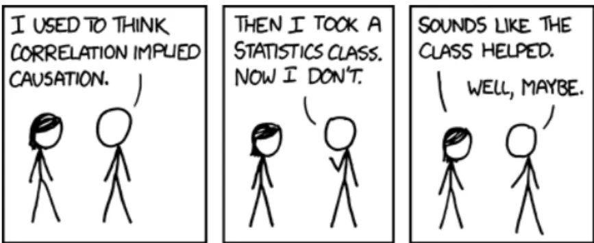
Figure 1-2: The risk of spurious correlation. Credit: xkcd.com
a more specific context to the study of this thesis, and close this non-quantitative introduction, we will introduce some important notions and concepts. Among them are the notions of un-supervised, supervised and semi-supervised learning, which describe the structure of the data with respect to the output.
1.1.4
Supervised, unsupervised and partially labeled learning
A great description of these three settings is provided in Wang and Summers (2012). In the supervised settings, there are two different types of data: inputs and outputs. The inputs are often named observations in Statistics and features in Machine Learning. The outputs are called outcomes in Statistics and labels in Machine Learning. The goal of Statistics in a supervised setting is to estimate a relationship between the inputs and the outputs. The relationship does not need to be a causal effect; it can be fortuitous (c.f. Figure 1-2). Most famous examples of supervised problems are the linear and non-linear regressions as well as the classification. Examples of supervised studies can be found in (Garcia et al.,2013; Bates et al.,
2014; Aphinyanaphongs et al., 2014; Tibshirani, 1996b).
The second setting is the unsupervised learning. In that case, there is no output in the sample, only inputs. The goal of unsupervised learning is to infer some relationships within the inputs. It is often assumed that there is an underlying latent variable that explains the relationship and behaviour of the observations. Well studied examples of unlabeled learning are density estimation, clustering and anomaly detection (Zeng et al., 2014; Le, 2013; Cheriyadat, 2014;
Zimek et al., 2014; Dinh et al., 2016; Costa et al., 2015;Gupta et al., 2014).
The partially labeled learning setting is an intermediate form of supervised learning. In that setting, some observations are associated with labels while other inputs have no corresponding outputs. The purpose of partially labeled learning is similar to the one of supervised learning,
which is to estimate a relationship between the inputs and the outputs. However, one may want to improve the quality of the estimation by using structural information of additional unlabeled features. Most of the time, semi-supervised learning is used when there are a few labeled data and a large amount of unlabeled data available. Within the partially labeled setting, two types of tasks might be considered. The semi-supervised learning tasks consist in estimating a predictor that minimizes a risk as in Equation1.2.3. On the other hand, the task of transductive learning is to predict the unknown outcomes of the unlabeled data that are within the original dataset. These settings will be further discussed in Chapter 4.
It is important to note that partially labeled learning differs from active learning. Active learning tasks consist of estimating a predictor from unlabeled data where an algorithm can request interactively the desired outputs of new data points in order to increase the quality of the estimate.
We have described the notions of supervised, non-supervised, and partially labeled learning, as well as semi-supervised, transductive and active learning tasks. In Chapter 4, we will consider the case of partially labeled setting and address some theoretical questions in the context of penalized regression.
In the next section, we will introduce some fields of statistical learning which are related to the work presented in this thesis. The goal of this section is to provide the reader with a global view of the literature related to our study. As this thesis is about theoretical statistics, we will mainly focus on papers that present an interest from the theoretical point of view. Besides, as it is at the intersection of many concepts, we believe it is worth going through a certain number of theories such as high-dimensional statistics, PAC-Bayesian estimation, aggregation, oracle paradigm, regularization and penalized regression. We will also discuss some theoretical results from the literature that address Monte Carlo computational challenges. It will nurture the last chapter of this thesis (Chapter 4).
1.2
Challenges in high-dimensional statistics
1.2.1
High-dimensional statistics
There has been a crucial shift of paradigm in the last decades. Let 𝑛 ∈ N be the number of observations and 𝑝 ∈ N be the number of features. The standard statistical framework considers the case where 𝑛 is relatively large and 𝑝 substantially smaller than 𝑛. As pointed out in Giraud (2014), the technological evolution of computing has urged a shift of paradigm
from classical statistical theory to high-dimensional statistics. In the high-dimension settings, a very large number of features 𝑝 is considered and the number of observations 𝑛 is of the same order of 𝑝, if not smaller.
The practical interest of the high-dimensional theory has come with the increasing number of data gathered by any connected object that can collect thousands to millions of different features. The paper Donoho (2000) gives a very clear overview of the particularities of high-dimensional statistics in comparison with classical statistics. This paper mentions that a very large number 𝑝 of features is not a blessing but a curse. Indeed, the very large number of features may sound like an opportunity to obtain a very thorough and complete quantity of information in order to infer or predict potentially anything. However, the difficulties in a high-dimensional settings are many. The computational challenge in a high-dimensional settings is of course one of the main concerns and supposes algorithms to be computable in polynomial time with respect to 𝑝 and 𝑛. In high-dimensional statistics, some methods priorize the computational complexity over the estimator optimality. For example, the optimal method to detect sparse principal components of high-dimensional variance-covariance matrix requires to solve a NP-complete problem. The authors of Berthet and Rigollet (2013) propose an alternative method that is nearly optimal in the detection level but guarantees the solution to be computable in polynomial time. In Chapter 4, we propose an algorithm to approximate a certain class of estimates and we prove that any targeted accuracy of the approximation can be reached in an explicit polynomial time.
In some situations, the high-dimensional context induces some heterogeneous collectin of data. A common situation is when a large dataset can be collected automatically at a low cost, while the label is difficult or costly to collect. In that case, it is relevant to collect a very large number of observations with no label and to manually collect labels associated with a few observations. This situation refers to partially labeled learning setting that we already mentioned earlier. This context will be discussed in the Chapter 3 and a review of partially labeled classification can be found in Schwenker and Trentin (2014) for further details on that matter.
On the other hand, some theoretical properties of the high-dimensional settings require to face other challenges. The survey Zimek et al. (2012) explains well the difficulty that a large value of 𝑝 induces when detecting outliers in a data set. This has strong consequences in high-throughput screening of molecules in the pharmaceutical industry, where the goal is to detect non-zero effect of a given feature as mentioned in the introduction of the bookBühlmann and Van De Geer (2011). Controlling false discovery becomes more difficult. A set of results on concentration inequalities is very useful to circumvent the challenge of controlling extreme
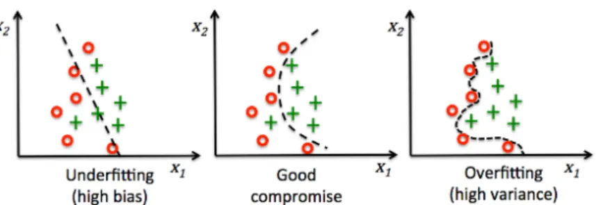
Figure 1-3: A representation (from left to right) of underfit-ting, balanced and overfitting classification learners. Credit: Python Machine Learning - Sebastian Raschka
values, when 𝑝 is large. The bookLedoux (2005) and the paperBoucheron et al.(2013) provide handy results on this matter.
Another famous phenomenon, when 𝑝 is relatively large, is the absence of property of conver-gence of the variance-covariance matrix estimation. For example, in the trivial case where 𝑛 random variables are sampled from a normalized Gaussian density of dimension 𝑝, 𝒩 (0𝑝, I𝑝), the
empirical covariance matrix does not converge almost surely toward the true covariance matrix which is the identity I𝑝 if 𝑝 is of the order of 𝑛 or larger. In the paperRavikumar et al. (2011),
a method is proved to be an appropriate estimator of the covariance in the high-dimensional settings.
Another theoretical challenge, and arguably the most famous, is the overfitting risk. As many features are available, it is tempting to use too many parameters to build an estimate relatively to the number of observations. However, if such an estimate has a very good fitting quality, the predictive risk on a new observation may be large. In that case the learning algorithm is said to have high variance. An excessively simplistic model has often high bias as it fails to model the actual connexion between the variables and the outcomes.
The overfitting phenomenon is widely discussed in the literature on different learning tasks such as regression (Hawkins, 2004;Hurvich and Tsai,1989), classification (Khoshgoftaar and Allen,
2001;Hsu et al.,2003) or outlier detection (Abraham and Chuang,1989;Pell,2000), and many methods have been developed such as cross-validation (Hsu et al., 2003; Refaeilzadeh et al.,
2009; Ng,1997), regularization (Tibshirani, 1996b;Bogdan et al.,2015; Zhang and Oles, 2001;
Bickel et al., 2009) or Bayesian prior (Cawley and Talbot,2007; Park and Casella, 2008; Wipf and Rao,2004) or pruning (Bramer, 2002). We will discuss some of these methods later in this thesis.
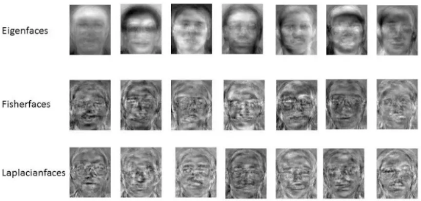
Figure 1-4: Various bases can be used to represent face images in order to approximate faces in a sparse representation. From top to bottom eigenfaces, fisherfaces and laplacianfaces are used. Credit: The Github repository Face Recognition from Wihoho -https://github.com/wihoho/FaceRecognition
settings: the sparsity. From a theoretical point of view, with no further assumptions, guarantees on estimation risk would be very difficult to prove. However, in empirical situations, it is very common to observe an underlying model that explains the generation of the data (from an inference point of view) or predict well the labels (from a predictive point of view) from a lower dimensional representation. Indeed, a lot of observed phenomena are in very high-dimensional settings but are actually governed by underlying patterns that can be explained in a much smaller dimension (at least approximately).
In signal processing, some sparse representations are infered using bases such as wavelets ( Mal-lat,1999).
1.2.2
Sparsity
Conceptually, the sparsity paradigm is far from being new. In the early 14th century, Occam
introduced the Occam’s razor principle5. The Occam’s razor is a principle making a
recom-mendation to choose among several possible explanations of a phenomenon. Occam suggests that it is best to choose the simplest possible model among the models that fit the observa-tions with a relative accuracy. In statistical terms, it means that among all the models that fit relatively well the dataset, it may be better to choose the simplest model. In high-dimensional statistics, the sparsity settings is a necessity. In Bühlmann and Van De Geer(2011), there is a rough expression of a condition on the sparsity level with respect to 𝑝 and 𝑛 required to achieve
Figure 1-5: An illustration of learning the empirical average of a face to increase robustness in image classification. Credit: Deric Bownd, Deric’s Mindblog
good estimation:
𝑠 log (𝑝) ≪ 𝑛, (1.2.1)
where 𝑠 is the sparsity level that will need to be defined. The definition of sparsity can differ according to the settings and the learning task. However, in many situations, there is an equivalence of the notion of sparsity.
For example, in the linear regression settings, the sparsity level is the number of non-zero para-meters. Let consider some data that consist of 𝑛 observations of random outcomes 𝑦1, . . . , 𝑦𝑛 ∈
R and 𝑝 fixed covariates 𝑥1, . . . , 𝑥𝑝 ∈ R𝑛. Let assume there is an unknown vector 𝛽⋆ ∈ R𝑝 such that the residuals 𝜉𝑖 = 𝑦𝑖− 𝛽1⋆𝑥1𝑖 − . . . − 𝛽𝑝⋆𝑥
𝑝
𝑖 are independent, zero mean random variables. In
vector notation, this reads as
𝑦 = X𝛽⋆+ 𝜉, (1.2.2)
where 𝑦 = (𝑦1, . . . , 𝑦𝑛)⊤ is the response vector, X = (𝑥1, . . . , 𝑥𝑝) ∈ R𝑛×𝑝 is the design matrix
and 𝜉 is the noise vector. For the sake of simplicity, let assume the noise vector to be distrib-uted according to the Gaussian distribution 𝒩 (0, 𝜎2I
𝑛), with 𝜎 a relatively small quantity in
comparison to the variance of the elements of 𝑦. If the quantity ‖𝛽⋆‖
0 of non null element of
𝛽⋆ is equal to 𝑠, then the linear model of 𝑦 admits a 𝑠-sparse representation with respect to the
features of the design matrix X. If 𝑠 is substantially smaller than the dimension 𝑝, it means that only a few features are explaining (or predicting) the outcome 𝑦.
Numerous patterns of sparsity exist. In order to describe the concept of sparsity in a general settings, we present the problem of regression in a general settings. Let consider the pair (𝑋, 𝑦) drawn from a distribution 𝑃 on a product space 𝒳 × 𝒴, we aim at predicting 𝑦 as a function of 𝑋. Mathematically speaking, we want to estimate a function 𝑓 : 𝒳 → 𝒴 that minimizes the
risk,
ℛ(𝑓 ) = ∫︁
𝒳 ×𝒴
𝑙(𝑦, 𝑓 (𝑥)) 𝑃 (d𝑥, dy), (1.2.3) where 𝑙 is an arbitrary loss function. We define 𝑓⋆ the function that minimizes Equation1.2.3.
The regression problem can then be written in the form
𝑦 = 𝑓⋆(𝑋) + 𝜉,
where 𝜉 ∈ R𝑝 is a vector of random variables. For example, if 𝑙 is the quadratic loss function,
then 𝑓⋆ is the Bayes predictor,
𝑓⋆(𝑥) = E[𝑦|𝑋 = 𝑥], and the noise 𝜉 is such that,
E[𝜉|𝑋] = 0𝑝. (1.2.4)
for any 𝛽 ∈ R𝑝. Then, the model admits a 𝑠-sparse representation if there exists 𝛽⋆
∈ R𝑝
such that 𝑓⋆ = 𝑓
𝛽⋆ and ‖𝛽⋆‖0 ≤ 𝑠. In the sparsity approach theory, the goal is to detect a
pattern within the data that can be approached with a sparse representation, but the linear representation may not be the right sparse representation. In the aforementioned case of linear regression, we consider a subset of functions 𝑓 such that 𝑓 can be written as a linear relationship betwen the data X and the label 𝑦,
𝑦 = 𝑓𝛽(X) + 𝜉 = X𝛽 + 𝜉, (1.2.5)
For example, in the task of piecewise constant regression, the goal is to estimate a piecewise constant function 𝑓 on a given interval 𝐼 defined by:
𝑓⋆(𝑥) =∑︁
𝑡∈𝑇
𝑐𝑡1𝑥>𝑡, (1.2.6)
where 𝑇 ⊂ 𝐼 is a finite set of elements. The goal of a piecewise constant regression task is to propose an estimation 𝑓 of the function 𝑓⋆ while we observe 𝑛 discrete random variables
(𝑦𝑖)𝑖∈[𝑛] such that
𝑦𝑖 = 𝑓⋆(𝑥𝑖) + 𝜉𝑖, (1.2.7)
where 𝑥𝑖 ∈ 𝐼.
If the set of rupture points 𝑇 is small, then there is a sparse structure in the model in the sense that there are very few variations. However, this is a different type of sparsity than in
the standard sparse linear model, since the support of the function 𝑓⋆ is not sparse. The sparse
regression of piecewise constant time series has been studied in numerous papers including (Bleakley and Vert,2011;Hocking et al.,2013;Antoch and Jarušková,2000). InGiraud(2014), several sparsity patterns are listed, including coordinate and variation6 sparsity, that we just
mentioned, but also group, sparse-group and basis sparsity that are important subjects in the literature (Reid,1982;Elad and Bruckstein,2002;Friedman et al.,2010;Meier et al.,2008). It is interesting to note that this typology of sparsity patterns can be generalized by remarking that they can all be considered as a sparse representation with respect to a specific representation. Indeed, let consider the noise-free oracle signal 𝑓⋆(X), all the aforementioned learning contexts
can be recasted as representing 𝑓⋆(𝑥
𝑖) = 𝑓𝑖⋆ as a scalar product between a given vector 𝛽⋆ and
a well suited basis 𝜓 of vectors (𝜓𝑖)𝑖∈[𝑛] such that 𝑓𝑖⋆ = ⟨𝛽⋆, 𝜓𝑖⟩ for any 𝑖 ∈ [𝑛]. Using this
representation, it is possible to define with consistence the notion of sparsity within a given basis.
Definition 1.2.1 (𝑠-sparsity). Let 𝑠 ∈ N, the signal 𝑙 = (𝑙(𝑥𝑖))𝑖∈[𝑛] is said to admit a sparse
representation with respect to 𝜓 if there exists a vector 𝛽⋆ ∈ R𝑝 such that ‖𝛽⋆‖
0 ≤ 𝑠 and
𝑙𝑖 = ⟨𝛽⋆, 𝜓𝑖⟩, (1.2.8)
for any 𝑖 ∈ [𝑛].
The parameter 𝑠 of Definition1.2.1may also be referred as the intrinsic dimension of a problem by some authors of the literature such as Guedj and Alquier (2013).
Since many regression problems can be recasted as a linear regression task, with respect to a given basis, we will only consider the linear case. Consequently, 𝑓⋆ will be represented by the
parameter 𝛽⋆ that we name the oracle parameter and we will make no distinction between the
data X and the basis 𝜑, with no loss of generality.
1.2.3
Prediction risk and oracle inequality
Unfortunately, the oracle is not known in practice. Indeed, the knowledge of 𝑓⋆ requires a
perfect information over the model. Therefore, one may need to estimate ̂︀𝛽 from the given observation (𝑦, X). It would be great to obtain guarantees on the risk of this estimator in the form
ℛ(𝑓𝛽̂︀) ≤ 𝐶, (1.2.9)
where 𝐶 ∈ R is a constant. Ideally, for a given estimate, this guarantee would hold in any condition, with very few assumptions with no dependency on the data X neither the noise 𝜉. Unfortunately, the prediction risk ℛ(𝑓𝛽̂︀) may differ from one problem to another. Indeed, 𝑓𝛽̂︀
is not the only parameter that plays a role on the risk. The level of noise 𝜉, and the level of information that X represents with respect to 𝑦, have both a strong impact on the risk. The smaller the noise to signal ratio, the smaller the risk can potentially be. From this point of view, the difficulty of the regression task differs. As a consequence, it is often impossible to obtain a guarantee of the quality of an estimator independently to the coherence of the model defined by the data X. Even though an absolute guarantee is not reasonable, it is possible, for some specific estimators, to compare the risk of the estimator to the risk of the oracle. This type of comparison is known in the literature as oracle inequalities and enables the guarantees of estimators to be studied with the consideration of the difficulty of a regression problem. The paper Candes (2006) reviews the powerful concept of oracle inequalities.
Definition 1.2.2 (Oracle risk inequality). Let 𝑓𝛽̂︀ be the prediction associated to the estimator ̂︀
𝛽 and let consider the regression problem defined in Equation 1.2.2, then the estimate ̂︀𝛽 is said to admit an oracle inequality with respect to an arbitrary loss function 𝑙, if there exists a constant 𝐶1 ∈ R and a function 𝐶2, depending on the model defined in Equation 1.2.2, such
that: 𝑙(𝑓 ̂︀ 𝛽, 𝑓 ⋆) ≤ 𝐶 1 inf 𝛽∈R𝑝{︀𝑙(𝑓𝛽, 𝑓 ⋆) + 𝐶 2(X, 𝜉)}︀. (1.2.10)
Furthermore, when 𝐶1 = 1, the oracle inequality is said to be sharp.
It is worth remarking that Inequality1.2.10 guarantees that there is no estimator 𝛽 ∈ R𝑝 that
is much better (in the sense of 𝐶2) than ̂︀𝛽. In particular, it implies that for any 𝛽 ∈ R𝑝,
𝑙(𝑓
̂︀
𝛽, 𝑓𝛽) ≤ 𝐶2(X, 𝜉). (1.2.11)
In particular, Inequality 1.2.11holds for 𝛽 = 𝛽⋆.
In that case, the inequality links the performance of the estimator ̂︀𝛽 to the performance of the oracle 𝛽⋆. The study of the quantity 𝐶
2 in Inequality1.2.10is of great interest, it is the rate of
convergence of the estimator ̂︀𝛽. In many cases, 𝐶2 decreases with the number of observations
𝑛 and increases with the variance 𝜎2 of the noise 𝜉 and with the dimension 𝑝. The optimality of the rate 𝐶2 is a well studied question in the literature of many estimators. Moreover, the
question of achieving a fast rate of the order 𝜎2log(𝑝)/𝑛 is a common benchmark in the linear
1.2.4
Oracle inequality in the sparsity context
In the context of the 𝑠-sparse assumption, one may consider all the supports with 𝑠 or less elements. In that case, the goal is to obtain a sparse estimator with a small risk. The 𝑠-sparse context is deeply studied in the literature (Bickel et al.,2009;Bellec et al.,2016b;Giraud,
2014). It is worth remarking that two types of results may be of interest with respect to the oracle inequalities. On the one hand, the first type of results are guaranteed provided that the true signal 𝛽⋆ is 𝑠-sparse. These results are said to consider well-specified learning tasks. On
the other hand, some results do not rely on the assumption of a well specified signal 𝛽⋆, this
is the notion of ill-specified oracle inequalities. In view of Definition1.2.2, well-specified oracle inequalities in the well specified case are of the form:
𝑙( ̂︀𝛽, 𝛽⋆) ≤ 𝐶1 inf 𝛽∈R𝑝𝑠
{︀𝑙(𝛽, 𝛽⋆) + 𝐶
2(X, 𝜉)}︀, (1.2.12)
where R𝑝
𝑠 is the set of 𝑠-sparse vectors of dimension 𝑝. This type of inequality guarantees that
the estimator performs nearly as well as any other 𝑠-sparse parameter. In the ill-specified case, this inequality has to hold for any 𝛽 ∈ R𝑝. Of course, the second case is more difficult to prove.
The function 𝐶2 is expected to be larger in the ill-specified case than in the well-specified case.
It is also of interest to quantify the degradation of this inequality when it is no longer a well-specified case. In the results of Chapter 2, we propose oracle inequalities that consider the ill-specified case and explicit the degradation of the inequalities due to the relaxation of the sparsity assumption.
In the sparse regression settings, with the belief that an unknown underlying sparse pattern represents the signal, or at least predicts an important portion of the signal, it is interesting to recover the sparsity pattern. Let 𝑆 be the support of the true parameter 𝛽⋆, the subset of non
null elements of 𝛽⋆, and let consider a computable loss criteria such as, for example,
ℓ𝑛(𝛽) = ‖𝑦 − X𝛽‖22, (1.2.13)
for any 𝛽 ∈ R𝑝; then, if 𝑆 was known, a good strategy would be to define the estimate as the
vector that minimizes Equation 1.2.13among all the vectors whose support is 𝑆. However, this under constraint minimization problem is not feasible since one does not know 𝑆. The task of selecting a model within a set of models 𝒮 often refers in the literature to the task of computing an estimate 𝑆̂︀ as an adequate support7. The best support among the set of support 𝒮 is the
oracle model.
Definition 1.2.3 (Oracle support). Let consider the problem of regression as defined in Equa-tion 1.2.2 and a loss function ℓ. Let 𝒮 be a set of supports in R𝑝. Then we define the Oracle
support with the set 𝒮 as
𝑆𝒮⋆ = arg min ¯ 𝑆∈𝒮E {︁ ℓ(︀𝛽⋆ , 𝛽⋆𝑆¯ )︀}︁ , (1.2.14) where 𝛽⋆ ¯
𝑆 is the best estimator with the support ¯𝑆. The unknown parameter 𝛽 ⋆
¯
𝑆 is the oracle
parameter on the support ¯𝑆.
Unfortunately, the oracle support cannot be calculated from the data since it relies on the unknown signal 𝛽⋆ and the unknown distribution 𝑃 . A possible approach is to estimate the
expected risk by an empirical loss function (such as 1.2.13) and define the estimated support such as ̂︀ 𝑆𝒮 = arg min ¯ 𝑆∈𝒮 {︁ ℓ𝑛 (︀ ̂︀ 𝛽𝑆¯)︀ }︁ , (1.2.15)
where ̂︀𝛽𝑆¯ is the estimate with support ¯𝑆 that minimizes the empirical risk ℓ𝑛(𝛽), as defined in
Equation 1.2.13.
After estimating a support 𝑆̂︀𝒮, an intuitive estimate of the regression problem would be ̂︀𝛽𝑆¯
as defined in Equation 1.2.15. However, such methods present a risk of bias. Indeed, the theoretical risk is likely to be underestimated when estimated with the empirical risk in the high-dimensional settings. This phenomenon is known under the name of overfitting. The empirical risk decreases with complex models that do not benefit from good properties on new data. In order to compensate this bias due to overfitting, some unbiased risk estimates have been proposed. These estimations combine an empirical loss function that measures the fitness of the parameter of the model and a penalty function that increases with the dimension of the selected model. Historically, some early penalization estimations of the risk have been proposed, such as the Akaike criterion:
̂︀
𝑆𝐴𝐼𝐶 = arg min ¯ 𝑆∈𝒮
{︀ℓ𝑛( ̂︀𝛽𝑆¯) + 2𝜎2‖ ̂︀𝛽𝑆¯‖0}︀. (1.2.16)
Even though the limits of the AIC estimator have been shown, it has opened the field of penal-ization methods that benefit from strong properties. More specifically, the AIC estimator can be seen as a maximum a posteriori estimator.
The remaining of this introductory chapter will give a brief overview of the litterature of res-ults on prediction by penalized (Section1.3) and averaged (Section1.4) estimators in fixed and we will focus on prediction tasks.