HAL Id: hal-00921674
https://hal.archives-ouvertes.fr/hal-00921674
Submitted on 20 Dec 2013
HAL is a multi-disciplinary open access
archive for the deposit and dissemination of
sci-entific research documents, whether they are
pub-lished or not. The documents may come from
teaching and research institutions in France or
abroad, or from public or private research centers.
L’archive ouverte pluridisciplinaire HAL, est
destinée au dépôt et à la diffusion de documents
scientifiques de niveau recherche, publiés ou non,
émanant des établissements d’enseignement et de
recherche français ou étrangers, des laboratoires
publics ou privés.
by Region Complexity
Petra Bosilj, Sébastien Lefèvre, Ewa Kijak
To cite this version:
Petra Bosilj, Sébastien Lefèvre, Ewa Kijak. Hierarchical Image Representation Simplification Driven
by Region Complexity. International Conference on Image Analysis and Processing, Sep 2013, Naples,
Italy. pp.562-571, �10.1007/978-3-642-41181-6_57�. �hal-00921674�
Hierarchical Image Representation
Simplification Driven by Region Complexity
Petra Bosilj1, S´ebastien Lef`evre1, and Ewa Kijak21 Univ. Bretagne-Sud, UMR 6074, IRISA, F-56000 Vannes, France
{Petra.Bosilj, Sebastien.Lefevre}@irisa.fr
2 Univ. Rennes I, UMR 6074, IRISA, F-35000 Rennes, France
Abstract. This article presents a technique that arranges the elements of hierarchical representations of images according to a coarseness at-tribute. The choice of the attribute can be made according to prior knowl-edge about the content of the images and the intended application. The transformation is similar to filtering a hierarchy with a non-increasing attribute, and comprises the results of multiple simple filterings with an increasing attribute. The transformed hierarchy can be used for search space reduction prior to the image analysis process because it allows for direct access to the hierarchy elements at the same scale or a narrow range of scales.
Keywords: hierarchical representation, tree structures, image filtering, segmentation and grouping, image region analysis
1
Introduction
Hierarchical image representations have been used in applications as diverse as object detection [22], video segmentation [11], image segmentation and filter-ing [1, 18], image simplification [16] and image compression [11]. They encode the composition of complex image structures by proposing the unions between simple image regions most likely to correspond to objects [22]. The choice of representation is application specific and is a compromise between representa-tion size and information retained by the representation elements [10, 22]. The organization these hierarchies reflects the inclusion relations between the regions and provides the means to detect and analyze objects at different levels of detail by examining the fine features present in small scale regions [10].
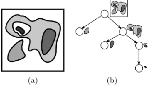
Among many equivalent representations used for such hierarchies (e.g. [1, 5, 7]), a representation by a tree structure is the direct one. Each node in such a tree corresponds to one of the regions in the representation, while the parent-child relations correspond to inclusions between regions (cf. Fig. 1).
A common property among all tree representations is that the leaf nodes represent the fine image structures, increasing in complexity with proximity to the root. The coarseness inherent to the representation could be defined as a distance from the node to the root of the tree. This inherent coarseness does
(a) (b)
Fig. 1.The tree in (b) is a hierarchical representation of (a)
not, in the general case, accurately reflect the region complexity and can not be used to compare any two regions. But, if some coarseness measure for the objects of interest is known prior to main image analysis step, the relevant search space could be limited to structures with a similar level of coarseness.
The transformation presented hereafter assigns an external coarseness mea-sure to all the nodes and rearranges them accordingly while preserving the hier-archical relations. New coarseness measure is chosen among increasing attributes on the tree, reflecting that the complexity of regions increases along each branch even if it can not be directly compared. The nodes of the same coarseness are pruned and at most one region of a certain coarseness per branch is kept. The result is a representation where the node levels correspond to the coarseness of the regions represented by the nodes and every tree level comprises only nodes of the same coarseness. This in turn enables limiting the search space when dealing with objects whose coarseness can be estimated by directly accessing only the regions of the relevant coarseness. Additionally, the search space is reduced even for objects with unknown coarseness, as the number of regions after the trans-formation can only decrease. This property makes the transtrans-formation suited for processing hierarchies that are too fine before the image analysis step.
In the next section, basic notions used throughout the article are introduced. Section 3 explains the effects of the proposed transformation, gives the algorithm and the estimation of the algorithm complexity. The approach is compared to previous works on the topic in Sect. 4, while the advantages and the potential applications of the presented algorithm are summarized in Sect. 5.
2
Properties of Tree Superclasses
In this section, we first offer a summary of some basic definitions about trees before discussing the differences between two superclasses, the partitioning and inclusion trees. Notations similar to the ones used here are used throughout literature (e.g. [14, 16]), and the reader can refer to these works for more details about directed and undirected graphs associated with image representations.
A tree T = (M, P ) can be defined as a directed graph, where M is the vertex (node) set and P the edge set of the graph. If there exists an edge em,nbetween
Complexity Driven Simplification of Hierarchical Image Representations 3
nodes without children are called leaf nodes. The only node in the tree with no parent is called the root. A path P in T from n1to nk is defined as (n1, . . . , nk)
such that for all 1 ≤ i < k, the node ni is a parent of ni+1. The vertex m is
called an ancestor of n if there exists a path P in T from m to n.
Let C = {n1, . . . , nk} be a set of nodes. C is a cut of the tree if every path P
from the root to any leaf passes through a single node nj∈ C. The level of the
root is the length of the longest path from the root to any of the leaves. Let n be any node in the tree except the root and ln the length of the path from the
root to n. The level of the node n is equal to the level of the root decreased by ln. A level of a tree is a cut in which all the nodes have the same level.
2.1 Trees as Hierarchical Image Representations
Let I be a monochannel digital image consisting of a set of pixels, f a function that assigns to each pixel p its intensity value, and G = (V, E) the associated undirected graph. The vertex set V contains all the pixels while the edge set E indicates their adjacency relation (cf. [14] for more details). In a tree T = (M, P ) corresponding to a hierarchical representation of I, every node n corresponds to a connected image region. The underlying graph R(n) of a connected region represented by the node n consists of a set of region pixels V (n) and the edge set E(n) = {ep,q∈ E|p, q ∈ V (n)} by the adjacency relation.
In such a representation the sets of pixels of two nodes are either disjoint, V(n) ∩ V (m) = ∅, or one of the nodes is an ancestor of the other. In case the node m is the ancestor of n, the following relation holds: V (n) ⊆ V (m). If m is a parent node in the tree and n1, . . . , nk are all the children of m, the edge set
of m can, in general case, be described as follows:
V(m) = V (n1) ∪ . . . ∪ V (nk) ∪ S, (1)
where S is a pixel set comprising pixels with the following property:
S= {p1, . . . , pl}, l ≥ 0 (2)
such that ∀i ∈ {1..l}, ∀j ∈ {1..k}, pi6∈ V (nj) .
Additionally, the pixel set S has to be such that the region R(m) = (V (m), E(m)) is a connected region in I. Additional constraints will be introduced when de-scribing trees from each of the superclasses. Despite the differences in inclusion order and types of regions dependent of the choice of tree, there are common properties within the superclasses, discussed hereafter.
2.2 Partitioning and Inclusion Trees
The common property among all partitioning trees is that the leaves corre-spond to regions of a fine partition of the image (e.g. initial over-segmentation [22], image flat zones [7, 10], watershed segmentation results [7]). Every cut of the tree is also a partition. Similarity between neighboring regions is either cal-culated based on a global similarity measure between region models (e.g. binary
partition tree [22]) or depends on local measures between neighboring pixels on the region borders (e. g. α-tree [7, 9, 16], alternate local measures [2, 17]). More similar regions are merged earlier in the construction process.
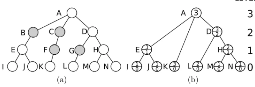
We will presume in this article that the tree is constructed with no redun-dancies, i.e. no two nodes represent the same region of the image I (the term is also used in [9] in the context of α-trees). For partitioning trees, this means that every inner node has strictly more than 1 child. If, due to the construction process, the same region appears multiple times in the hierarchy, we will simply say that the node representing it appears on multiple levels without duplicating the node. Instead of just a level, we assign a level range [lMin, lMax ) to the node. lMinand lMax are then defined as the lowest levels in the tree on which the node does and does not appear on, respectively. The maximal level of a node is equal to the minimal level of its parent. The root node is the exception, existing only on the maximal level present in the tree. Representing a tree with redundancies as a tree without them results in no loss of information (illustrated in Fig. 2).
Since the leaf nodes already form an image partition, no new pixels are added when constructing a parent node. Any inner region is a union of at least two of its children. Partitioning trees with no redundancies can be formalized by adding the constraint k > 1 in (1) and l = 0 in (2).
For inclusion trees, no explicit measure defining the merging order is pre-sent. Leaves in these trees are either image intensity maxima, minima, or both, and do not form a partition of the image. Level sets [4, 19] of an image are ob-tained by thresholding the image, and looking at connected components formed by pixels p with intensities f (p) above (for upper level sets) or below the thresh-old (for lower level sets). Inclusion trees are built based on inclusion relations between the level sets of the same type (min- and max-trees [3, 6]) or of both types (level line trees [4, 19, 21], dual-input max-trees [8]).
We also presume no redundancies in the inclusion trees, which in this context means that a region not represented by a leaf node can only be formed by adding, to an existing region (or regions), the pixels of one or more flat zones not included in the region(s) yet. Flat zones [13] of an image I are connected regions of same intensity pixels with maximal size. The set of pixels of an inner node can not be formed by merging multiple child regions without adding new pixels. All the construction algorithms for commonly used inclusion hierarchies produce inclusion trees with no redundancies as their output [4, 6, 19]. The only constraint to add to the general definition of tree hierarchies is l > 0 in (2).
3
The Proposed Transformation
The algorithm for imposing an external coarseness measure on a tree represen-tation of an image without redundancies is presented in this section. The output is also a tree representation with no redundancies, whose levels comprise nodes with the same value of the coarseness measure.
The first assumption of the algorithm, explained already in Sect. 2.2, is that the tree representation is without redundancies. The second condition pertains
Complexity Driven Simplification of Hierarchical Image Representations 5 A D E H K L M N J B C F G I (a) N A D E H K L M J I
3
2
1
0
LEVEL: 3 2 2 1 3 0 3 1 1 0 10 20 10 10 3 (b)Fig. 2.The tree shown in (a) has redundant nodes, marked in gray. The levels of the nodes are displayed on the right of the trees. By removing the redundancies we get the tree shown in (b) (the level range [lMin, lMax ) is displayed inside the nodes).
to the attribute K(·) used as a new coarseness measure for regions. An attribute K(·) is said to be increasing [14] on a tree if the attribute value of a parent m node is always greater than or equal to the attribute values for all its children ni: K(m) ≥ K(ni).The coarseness measure used must be an increasing attribute
(discussed in Sect. 1), and the algorithm assumes that the values of this increas-ing attribute were assigned to the nodes of the tree before the transformation. Many interesting attributes (e.g. intensity range, component area) can be as-signed to nodes directly during tree construction. More attribute possibilities can be found in [12, 15], but the final choice always depends on the intended application and known properties of object of interest and image domain.
Transformation results can be interpreted as a hierarchy formed by stacking, for threshold values ranging from zero to maximal value of the attribute, the leaf nodes of trees obtained by performing attribute filtering [12] on the original tree with an increasing attribute. The result is a tree representation of this hierarchy with no redundancies. A node present as a leaf in the hierarchy after an attribute filtering with a threshold T will have T included in its level range in the result. After the transformation, the tree cuts stacked to produce a new tree can be directly accessed. This definition extends easily to attributes that take continuous values, where the node can belong to a continuous range of levels.
3.1 The Algorithm
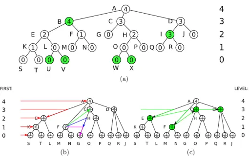
Assuming no redundancies and that the attribute values are already calculated for every node, the algorithm can be described in very simple terms: in a bottom-up traversal of the tree, if we discover a node with an attribute value equal to the attribute value of its parent, we should add all the child-nodes of this node to the children set of its parent, and then delete the node. This is summarized in Algorithm 1. The attribute value assigned to a node in the original tree becomes the minimal level of that node if the node is kept after the transformation. The tree before and after the transformation is shown in Fig. 3(a) and 3(b).
If the tree is stored in the straightforward way, the memory requirements are proportional to number of image pixels (c.f. Sect. 3.2). Highest cut of the
1 function rearrangeTree(Node): 2 foreach Child∈ Node.children do
3 rearrangeTree(Child)
4 if Node.attributeValue= Node.parent.attributeValue then 5 add Node.childrento Node.parent.children
6 delete Node
7 else
8 Node.minLevel← Node.attributeValue
9 Node.maxLevel← Node.parent.attributeValue
Algorithm 1: The proposed transformation
tree comprising nodes with coarseness lower or equal to the desired level is then selected by performing a top-down traversal of the tree and keeping the first node in each branch with satisfying coarseness level. Memory requirements rise if we want faster access. For each level of the tree we store a pointer to the left-most node and, for each node and each level in the level range of the node, the first next node at that level in the tree. Figures 3(b) and 3(c) illustrate the information which needs to be stored to enable direct access to any tree level. Once the first node in a level of a tree is accessed, the pointers to the next nodes can be followed to access all the nodes of that level.
3.2 Complexity Analysis
From the pseudocode, it is visible that the algorithm is linear in the number of nodes in the tree. In order to estimate the complexity of the algorithm, we must estimate the maximum number of tree nodes in a tree T = (M, P ) with no redundancies, compared to the number of pixels N in the image I with the corresponding graph G = (V, E), where N = card (V ). The estimation is done separately for partitioning and inclusion types of trees.
The maximum number of leaves in a partitioning tree is achieved if the elements of the finest partition represented by the tree are pixels. Since the tree has no redundancies, every inner node in the tree has at least 2 distinct child nodes. The number of inner nodes is less or equal than that of a binary tree with the same number of leaves, and never exceeds the number of leaves in the tree. There are at most N leaves, so the maximum number of nodes in any partitioning tree is lower than 2N .
The maximum number of nodes in an inclusion tree is achieved if every node adds the smallest possible number of pixels, i.e. 1 pixel, to the region it represents. As there are no overlaps between the regions of different branches, each pixel in the image can be added to the set of region pixels exactly once. Regardless of the number of leaf nodes in the inclusion tree and given that there are N pixels in the image, there can be at most N nodes in any inclusion tree.
Considering that the number of nodes in any tree image representation with-out redundancies is linear in the number of image pixels and the transformation
Complexity Driven Simplification of Hierarchical Image Representations 7 N P Q
4
3
2
1
0
LEVEL: A B C D E F G H I J K L M O R S T U V W X 4 4 3 3 3 2 1 2 1 0 0 0 0 0 0 0 0 0 0 0 0 0 0 0 (a) A C D E H K F S T L M N G O P Q R J 4 3 3 2 3 0 20 20 30 30 4 3 1 0 10 4 1 2 0 1 0 4 2 2 1 1 0 4 3 0 4 3 2 1 0 FIRST: (b) A C E H K F S T L M N G O P Q R J D 4 3 3 2 3 0 20 20 30 30 4 3 1 0 10 4 1 2 0 1 0 4 2 2 1 1 0 4 3 0 4 3 2 1 0 LEVEL: (c)Fig. 3.Subfigure (a) shows the original tree before the transformation, with attribute values displayed in the nodes and the nodes to be removed highlighted in green. In both subfigures (b) and (c), the level range is displayed inside the nodes. Subfigure (b) shows pointers to beginning of every tree level, needed for direct access to levels. Entries like the one shown for node F keep the next node for every level [1, 4i (level 1: G(purple), 2: G (blue), 3: C (green)) and need to be stored for every node. Subfigure (c) shows accessing the third level of the tree using the stored pointers.
algorithm is linear in the number of tree nodes, we can conclude that the com-plexity of the algorithm is linear in the number of image pixels, O(N ). The overall complexity of producing such a transformed tree from the original im-age depends on the choice of the original underlying tree, the complexity of the construction algorithm for the chosen tree type and additional costs (if any) of calculating node attribute values.
4
Similar Approaches
The search through the literature for alternate approaches to selecting the coars-est tree-cut satisfying some constraint found such attempts only in the domain of partitioning trees. Imposing constraints on components of another partitioning hierarchy in a way that the hierarchical relations between the remaining com-ponents are preserved was first explored in [15]. The work in [15] only provides the definitions of constrained components and the potential applications while the algorithm for selecting such constrained components is not proposed.
The approaches presented in [5, 9] were demonstrated on α-trees, but are applicable to all partitioning trees. Due to the definition of α-connectivity, the α-connected components suffer from the chaining effect [17,18]. This effect causes some nodes close to the leaves of the tree to be complex regions instead repre-senting the fine details of the image. Because of this, the concept of constrained connectivity was introduced [16] together with the notion of an (ω)-hierarchy by imposing global component range constraints on α-connected components. This component range constraint can be viewed as an external coarseness measure.
In [9], the approach to extract just one level of the (ω)-hierarchy at a time is presented. Their approach for creating the desired partition is equivalent to the process of attribute filtering (with an increasing attribute) [12] on the hi-erarchical image representation, but they only use the leaf nodes of the filtered hierarchy. The algorithm presented herein was inspired by the idea from [9] and adopted its bottom-up approach to tree traversal. The difference is that stopping the tree traversal as soon as the attribute values are above the chosen threshold, as in [9], returns only one partition, while continuing the traversal to the root of the tree as proposed here builds a structure containing the information on partitions for every possible threshold value. The algorithm presented here can be compared to the direct rule of simplifying the tree with a non-increasing crite-rion [11]. The critecrite-rion for keeping the node is that the attribute value assigned to it is strictly smaller than that of its parent.
The main contribution of [5] is a representation of partitioning tree hierar-chies in the framework of edge-weighted graphs, proving that any partitioning hierarchy can be represented by an ultrametric watershed. They present an al-gorithm to calculate the ultrametric watershed representation for any hierarchy by imposing an increasing constraint on the initial hierarchical segmentation. Applying the constraints on the original hierarchy is linear in the number of image pixels and the complexity, O(N ), is commensurable with the complexity of the algorithm presented in this article. Similarly to the algorithm presented here, the overall complexity of calculating a hierarchical segmentation based on constrained connectivity as presented in [5] depends on the complexity of calculating the original hierarchy and calculating the attribute values for each of the original tree components. However, since [5] is operating on ultrametric watersheds, their approach is not applicable to inclusion trees.
5
Discussion and Conclusion
Applying additional constraints on a hierarchical partitioning of an image is already well explored in [5, 9, 15]. The earliest works on the topic [15] suggest varying the constraint threshold parameters to control the degree of image sim-plification. When the node level does not coincide with the perceived complexity of the represented region (e.g. the chaining effect in α-trees), applying constraints rearranges the hierarchy according to a more precise external coarseness mea-sure [9,15]. The results can also be interpreted as performing an attribute filtering with all threshold values simultaneously and storing all the results within a same
Complexity Driven Simplification of Hierarchical Image Representations 9
structure [9]. In image segmentation, regions of a hierarchical image partition are treated as “puzzle pieces” [15, 16] used to compose a segmentation. The trans-formation reduces hierarchy size, lowering the number of “puzzle choices” and simplifying the calculation of the segmentation. Binary partition trees used for object detection [22] generate partitions so fine that a second merging criterion is used in order to generate a coarse partition in which the potential detections are marked before the object can be detected in the fine parts of the hierarchy. By reducing the size of the hierarchy, better detection could be achieved by using more complex algorithms or a more exhaustive search.
In the domain of inclusion trees, many applications would benefit of the reduction in the search space. Finding the k most prominent structures in an image (cf. [6]) depends directly on the size of the tree. Transforming an inclusion hierarchy simplifies the image in a way similar to the one presented in [15] for partitioning trees. The image simplification technique using level line trees pro-posed in [4], based on area size, can also be applied to a hierarchy first simplified using a different coarseness attribute. An image comparison method proposed in [4] relies on assigning attributes to describe the regions of the hierarchy and then checking one of the images for presence of shapes similar to shapes present in the other image. Since the method is already working by finding similar (and not the same) shapes, a simplification of hierarchies before image comparison would reduce the overall number of comparisons speed up the process. The be-ginnings of using hierarchical image representations in content-based image re-trieval rely on examining image structural elements corresponding to the nodes in the tree [21] and would also benefit from the reduction in hierarchy size. As the approach to background detection presented in [20] depends on the values of several thresholds, multiple precision results could be obtained simultaneously by applying the presented transformation instead of a simple tree filtering only. This article presented a technique which imposes an external coarseness mea-sure on hierarchical image representations, applicable to both partitioning and inclusion trees. In addition to solving the problem for a larger class of hierarchies than [5], the proposed approach is intuitive and simple to implement and oper-ates on the direct representations of image hierarchies – the tree representations. Many potential applications listed provide interesting directions for future work, taking advantage of the transformation going a step further in search space size reduction compared to directly using hierarchical image representations.
References
1. Cousty, J., Najman, L.: Incremental Algorithm for Hierarchical Minimum Spanning Forests and Saliency of Watershed Cuts. In: Soille, P., Pesaresi, M., Ouzounis, G.K. (eds.) ISMM 2011. LNCS, vol. 6671, pp. 272–283. Springer, Heidelberg (2011) 2. Gueguen, L., Soille, P.: Frequent and Dependent Connectivities. In: Soille, P.,
Pesaresi, M., Ouzounis, G.K. (eds.) ISMM 2011. LNCS, vol. 6671, pp. 120–131. Springer, Heidelberg (2011)
3. Jones, R.: Connected Filtering and Segmentation using Component Trees. Com-puter Vision and Image Understanding 75(3), 215–228 (1999)
4. Monasse, P., Guichard, F.: Fast Computation of a Contrast-Invariant Image Rep-resentation. IEEE Transactions on Image Processing 9(5), 860–872 (2000) 5. Najman, L.: On the Equivalence Between Hierarchical Segmentations and
Ultra-metric Watersheds. JMIV 40(3), 231–247 (2011)
6. Najman, L., Couprie, M.: Building the Component Tree in Quasi-Linear Time. IEEE Transactions on Image Processing 15(11), 3531–3539 (2006)
7. Najman, L., Soille, P.: On Morphological Hierarchical Representations for Image Processing and Spatial Data Clustering. In: K¨othe, U., Montanvert, A., Soille., P. (eds.) WADGMM 2010, LNCS, vol. 7346, pp. 43–67. Springer, Heidelberg (2012) 8. Ouzounis, G., Wilkinson, M.: Mask-Based Second-Generation Connectivity and
Attribute Filters. IEEE Transactions on Pattern Analysis and Machine Intelligence 29(6), 990–1004 (2007)
9. Ouzounis, G.K., Soille, P.: Pattern Spectra from Partition Pyramids and Hierar-chies. In: Soille, P., Pesaresi, M., Ouzounis, G.K. (eds.) ISMM 2011. LNCS, vol. 6671, pp. 108–119. Springer, Heidelberg (2011)
10. Salembier, P., Garrido, L.: Binary Partition Tree as an Efficient Representation for Image Processing, Segmentation, and Information Retrieval. IEEE Transactions on Image Processing 9(4), 561–576 (2000)
11. Salembier, P., Oliveras, A., Garrido, L.: Antiextensive Connected Operators for Image and Sequence Processing. IEEE Transactions on Image Processing 7(4), 555–570 (1998)
12. Salembier, P., Wilkinson, M.H.F.: Connected Operators. IEEE Signal Processing Magazine 26(6), 136–157 (2009)
13. Serra, J.C., Salembier, P.: Connected operators and pyramids. In: Dougherty, E.R., Gader, P.D., Serra, J.C. (eds.) Image Algebra and Morphological Image Processing IV. SPIE, vol. 2030, pp. 65–76. SPIE Press, San Diego (1993)
14. Soille, P.: Morphological Image Analysis: Principles and Applications. Springer-Verlag, New York, second edn. (2003)
15. Soille, P.: On Genuine Connectivity Relations Based on Logical Predicates. In: Proc. of 14th Int. Conf. on Image Analysis and Processing. pp. 487–492. IEEE Computer Society Press, Los Alamitos (2007)
16. Soille, P.: Constrained Connectivity for Hierarchical Image Partitioning and Sim-plification. IEEE Transactions on Pattern Analysis and Machine Intelligence 30(7), 1132–1145 (2008)
17. Soille, P.: Preventing Chaining Through Transitions While Favouring It within Homogeneous Regions. In: Soille, P., Pesaresi, M., Ouzounis, G.K. (eds.) ISMM 2011. LNCS, vol. 6671, pp. 96–107. Springer, Heidelberg (2011)
18. Soille, P., Grazzini, J.: Constrained Connectivity and Transition Regions. In: Wilkinson, M.H.F., Roerdink, J.B.T.M. (eds.) ISMM 2009. LNCS, vol. 5720, pp. 59–69. Springer, Heidelberg (2009)
19. Song, Y.: A Topdown Algorithm for Computation of Level Line Trees. IEEE Trans-actions on Image Processing 16(8), 2107–2116 (2007)
20. Song, Y., Zhang, A.: Locating Image Background By Monotonic Tree. In: Caulfield, H., Chen, S.H., Cheng, H.D., Duro, R., Honovar, V., Kerre, E.E., Lu, M., Romay, M., Shih, T., Ventura, D., Wang, P., Yang, Y. (eds.) 6th Joint Conf. on Information Sciences. pp. 879–884. Association for Intelligent Machinery, Inc., Durham (2002) 21. Song, Y., Zhang, A.: Analyzing scenery images by monotonic tree. ACM
Multime-dia Systems J. 8(6), 495–511 (2003)
22. Vilaplana, V., Marques, F., Salembier, P.: Binary Partition Trees for Object De-tection. IEEE Transactions on Image Processing 17(11), 2201–2216 (2008)