HAL Id: hal-01241470
https://hal.inria.fr/hal-01241470
Submitted on 10 Dec 2015
HAL is a multi-disciplinary open access
archive for the deposit and dissemination of
sci-entific research documents, whether they are
pub-lished or not. The documents may come from
teaching and research institutions in France or
abroad, or from public or private research centers.
L’archive ouverte pluridisciplinaire HAL, est
destinée au dépôt et à la diffusion de documents
scientifiques de niveau recherche, publiés ou non,
émanant des établissements d’enseignement et de
recherche français ou étrangers, des laboratoires
publics ou privés.
Closed-Loop Autofocus Scheme for Scanning Electron
Microscope
Le Cui, Naresh Marturi, Eric Marchand, Sounkalo Dembélé, Nadine Piat
To cite this version:
Le Cui, Naresh Marturi, Eric Marchand, Sounkalo Dembélé, Nadine Piat. Closed-Loop Autofocus
Scheme for Scanning Electron Microscope. Int. Symp. of Optomechatronics Technology, ISOT 2015,
Oct 2015, Neuchatel, Switzerland. �10.1051/matecconf/20153205003�. �hal-01241470�
© Owned by the authors, published by EDP Sciences, 2015
Closed-Loop Autofocus Scheme for Scanning Electron
Mi-croscope
Le Cui1,a, Naresh Marturi2, Eric Marchand1, Sounkalo Dembélé2, and Nadine Piat2
1Université de Rennes 1, Lagadic team, IRISA, Rennes, France 2
AS2M department, FEMTO-ST institute, Besançon, France
Abstract. In this paper, we present a full scale autofocus approach for scanning electron
micro-scope (SEM). The optimal focus (in-focus) position of the micromicro-scope is achieved by maximizing the image sharpness using a vision-based closed-loop control scheme. An iterative optimization algorithm has been designed using the sharpness score derived from image gradient information. The proposed method has been implemented and validated using a tungsten gun SEM at various experimental conditions like varying raster scan speed, magnification at real-time. We demonstrate that the proposed autofocus technique is accurate, robust and fast.
1 Introduction
For high accuracy during manipulation tasks or micro-nanoscale measurements under a scanning elec-tron microscope (SEM), high quality and sharp im-ages are always required. For this purpose, an effi-cient and reliable SEM autofocus algorithm has to be executed before the manipulation process. In general terms, autofocus is a process of maximizing the image sharpness by regulating the device focus sets. There are two types of autofocus techniques: active meth-ods, using a different subsystem to modify the lens po-sition and passive methods, which solely rely on the image sharpness information. Out of the two, pas-sive methods are commonly employed for microscopic
devices. Since the geometry and projection model
of a SEM are different to optical systems [1, 2], the autofocus process is different. Most of the autofocus methods are based on evaluating the image sharpness score i.e., the score should reach a single optimum of a selected sharpness function at the in-focus image. For this purpose, many sharpness criteria such as im-age variance, autocorrelation, wavelets, Fourier trans-form were discussed for microscopic applications [3]. A comparison of these criteria regarding electron mi-croscopy was discussed in [4].
To perform passive autofocus process with SEM, a former method is to obtain a sequence of images within a defocus range and to compute their sharp-ness scores. The optimal SEM focal length that cor-responds to the maximum of sharpness score is then obtained [5]. The main drawback in this approach
ae-mail: [email protected]
is that it requires the acquisition of many images, which is practically time consuming due to the high focus range of SEM. Alternatively, a later method is to start with an initial set of SEM imaging param-eters that correspond to a defocus image. Then an iterative algorithm is used to search for the best fo-cus position [6, 7]. Even though these methods are effective, they are highly dependent on the search his-tory. Rudnaya [8] has proposed to use Nelder–Mead method for searching the optimum of image variance. An alternative method has been proposed in [9], based on fitting the sharpness function to a quadratic poly-nomial approximatively using some initial measure-ments. In [10], the autofocus has been achieved by computing the derivative of sharpness function nu-merically. Finally, statistical learning-based autofo-cus methods were studied for SEM [11], but were never implemented in real-time.
In this paper, we consider the autofocus issue as a control problem and propose a direct closed-loop con-trol scheme to solve it. The objective is to concon-trol the device focal length (working distance) iteratively based on the time variation of the gradient informa-tion of acquired image. An analytical formulainforma-tion of the relation between the displacement of the work-ing distance and the variation of the gradient infor-mation is proposed. The considered method advances the available methods in different ways. First, It over-comes the problem of hysteresis since it is independent of the search history and directly reaches the optimal focus position. Next, the method automatically cir-cumvents unnecessary defocus positions that makes it faster than the search-based techniques. Finally,
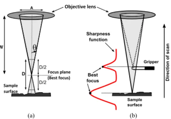
The Journal’s name W D D/2 D/2 Objective lens Focus plane Sample surface A (Best focus) θ (a) Best focus Sample surface Direction of scan Sharpness function Gripper (b)
Figure 1. (a) SEM focusing geometry (b) sharpness
func-tion variafunc-tion.
since analytic formulation of derivative has been com-puted, the algorithm is more robust w.r.t numerical computation- or regression-based method. We deem these important, if the method needs to be integrated with any other real-time tasks.
2 Background on SEM Focusing
2.1 SEM Focusing GeometryIn general, the SEM images are formed by scanning a sample surface by means of a focused beam of high en-ergy electrons. Different sets of electromagnetic lenses in the SEM electron column are responsible for per-forming the focusing task. The first are the condenser lenses that control the beam diameter and the second are the objective lenses that focus the spot sized beam on to the sample surface. Apart from them, an objec-tive aperture is present in between them to filter out the non-directional electrons. The distance measured electronically between the final pole piece of the objec-tive lens and the focal plane is the electronic working distance W (focal length), which plays a vital role in the focusing process. This distance depends on two factors: the beam acceleration voltage and the cur-rent passing through the objective lens. In this work, we assume the former remains constant and the main focusing is performed only using the latter. The total focusing process is illustrated in the Fig. 1(a). For any
selected magnification, at a distance D2 on both sides
of the focal plane, the beam diameter is two times pixel diameter. This results in the images that look to be acceptably in-focus.
2.2 SEM Image Formation
The general image formation model, which is com-monly used in the case of optical microscopes [12], can be extended to use with a SEM [11]. Consid-ering an extremely small area element dxdy centered on (x, y), the secondary electron (SE) current emitted from this area is
ds(x, y) = δ(x, y)ϕ(x, y)dxdy, (1)
where, ϕ(x, y) is the incident current density at the point (x, y), δ(x, y) is a yield coefficient which is
as-Control law SEM Vision displacement PC SEM SEM focus control image gradient working distance input error
Figure 2. Control framework for SEM autofocus
signed in a way that δ is the average number of
re-sultant secondary electrons emitted. The total SE
current emitted from the specimen s is, s = Z ∞ −∞ Z ∞ −∞ δ(x, y)ϕ(x, y)dxdy. (2)
Considering an approximative linear relation between emitted SE current s and the result signal i (i.e. i(x, y) = ks(x, y), k is a constant), the SEM im-age formation can be seen as a linear convolution of a specimen-dependent component and a system-dependent point-spread function (PSF) [5, 11]. Here, the PSF is the scaled and reflected electron beam cur-rent density passing through the origin. Considering this, the result image i(x, y) can be expressed as the
convolution of an in-focus image i∗(x, y) with a
defo-cus kernel h(x, y) and is given by
i(x, y) = i∗(x, y) ∗ h(x, y) (3)
Previous studies state that, a Gaussian kernel can be used as an approximation to the defocus kernel [13]. In this case, the probability density function (PDF) is given by
h(x, y) = 1
2πσ2e
−x2 +y2
2σ2 . (4)
where, σ is the standard deviation of the Gaussian kernel.
3 Closed-Loop Control Scheme for SEM
Autofocus
As mentioned before, autofocus can be achieved by computing the maximum value of the sharpness func-tion (see Fig. 1(b)). In the proposed approach, the autofocus process is regarded as a closed-loop control problem where the focal length of SEM is updated at each iteration until the optimal focus is reached (see Fig. 2). In this section, we will first show how to use the image gradient for a closed-loop control scheme (in case of parallel projection). Then we derive the control law to perform the autofocus task.
3.1 Sharpness Function for Closed-Loop Control Previously, it has been shown that the gradient-based sharpness measures perform well with electron
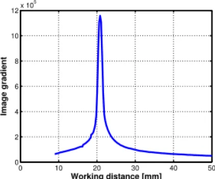
0 10 20 30 40 50 0 2 4 6 8 10 12x 10 5 Working distance [mm] Image gradient
Figure 3. Evolution of image gradient with respect to
working distance.
use image gradient is that it shows a good compro-mise in the case of unstable image contrast, which has to be considered with SEM [14]. Besides, in [15] it has been proposed to use image gradient informa-tion to perform vision-based posiinforma-tioning tasks and a similar process could be envisioned for an autofocus task. However, due to the parallel projection model at high magnification which is inherent to a SEM [2], the perspective projection-based control law proposed in [15] cannot be employed for the SEM. To tackle this problem, we propose in this section a direct projection model-free approach to derive the control law for full scale autofocus.
Considering the fact that the image gradient varies when the image focus changes i.e., when the working distance varies, we aim to update the working distance by a closed-loop control law to obtain the maximum of image gradient. For an acquired image i(x, y), the squared norm of the gradient g(x, y) at a point (x, y) is expressed by
g(x, y) = k∇i(x, y)k2= ∇i2x(x, y) + ∇i2y(x, y) (5)
where, ∇i2x(x, y) and ∇i2y(x, y) represent the
squares of gradient in x and y directions, respectively. Considering the squared norm of the gradient G for a whole image (size M × N ) as the sharpness function to be maximized by varying W , we have
ˆ W = arg max W G(W ) (6) where G(W ) = M X x=0 N X y=0 g(x, y, W ) = M X x=0 N X y=0 (∇ix2(x, y, W ) + ∇iy2(x, y, W )). (7) Here instead of extracting any local features, a global feature G is defined over a whole image. Fig. 3 shows the variation of image gradient G for a series of SEM electronic working distances. In fact, it is not nec-essary to take into account any local information(i.e. shape, texture and uniformity of the sample), since the image gradient for most of the pixels increases (or
decreases) when changing working distance, resulting a smooth sharpness function which has one evident optimum (at the desired working distance). Consid-ering the autofocus task as a closed-loop control law, the objective is to compute the variations of the
work-ing distance ˙W from the variation of G for achieving
an optimal SEM focus set.
In order to employ image gradient information as the sharpness function for full scale in a SEM, the relation between the temporal variations of working distance W and image gradient G is considered:
˙
G = JGW .˙ (8)
The Jacobian JG that links the variations of
work-ing distance W and image gradient G in (8) can be expressed by JG = ∂G ∂σ ∂σ ∂W (9)
where, σ is the standard deviation of Gaussian kernel given in (4). For a small displacement of W , con-sidering a proportional relation between σ and W ,
∂σ ∂W = k, leading to JG = ∂G ∂W = k ∂G ∂σ (10) From (7), ∂G ∂σ can be expressed as ∂G ∂σ = M X x=0 N X y=0 2(∇ix(x, y) ∂∇ix(x, y) ∂σ + ∇iy(x, y) ∂∇iy(x, y) ∂σ ). (11)
Next, (3) can be rewritten as follows:
i(x, y) =X
m
X
n
i∗(x − m, y − n)h(m, n). (12)
From (4), we get the derivative of the Gaussian kernel: ∂h(m, n) ∂σ = 1 2π(m 2+ n2− 2σ2)σ−5e−m2 +n2 2σ2 (13)
Considering (12) and (13), we have
∂∇ix(x, y) ∂σ = X m X n ∇(i∗x(x − m, y − n) · 1 2π(m 2+ n2− 2σ2)σ−5e−m2 +n2 2σ2 ) (14) and ∂∇iy(x, y) ∂σ = X m X n ∇(i∗y(x − m, y − n) · 1 2π(m 2+ n2− 2σ2)σ−5e−m2 +n2 2σ2 ) (15) Replacing (14) and (15) in (11), we can finally
The Journal’s name 3.2 Control Law
The objective of our approach is to maximize the G by controlling the working distance W to obtain an optimized focus of SEM. In order to maximize G, we are going to minimize a cost function given by
ε(W ) = αe−βG(W )− γ (16)
where, α, β ∈ R+ are adaptive gains that control the
variation of working distance and the speed of
con-vergence. γ is a small positive value that can be
considered as a threshold to determine if the opti-mal focus is reached. The algorithm will stop when αe−βG(W )6 γ. Considering an exponential decrease
of the error i.e., ˙ε = −λε, the control law is:
ξ = −λJε−1ε (17)
where, ξ is the velocity along the focal axis and Jε is
the Jacobian and can be expressed by
Jε=
∂ε ∂W
= −(ε + γ)βJG. (18)
Rewriting (17) using (18), leads to
ξ = λε
(ε + γ)βJG
(19) Subsequently, the W displacement (working distance) to be set with the SEM has been computed as follows
∆W = ξ∆t (20)
where, ∆t is the time taken between the two acquired images. For each iteration, the working distance is updated as given by
Wnew=
(
Wprev− |∆W | if W0 close to Wmax
Wprev+ |∆W | if W0 close to Wmin
(21)
where Wnew is the working distance to be updated,
Wprev and W0 are previous and initial working
dis-tances, respectively, |∆W | is the magnitude of ∆W ,
Wmax = 50 and Wmin = 1 are the factory
pro-vided maximum and minimum values for the elec-tronic working distance (in mm) of the employed SEM, respectively. In our experiments, (21) is used to control the direction of displacement computed by the control law. For the initial working distance close to a middle value between 1 and 50, according to the single maximum in the evolution of image gradient
with respect to working distance (see Fig. 3), the
direction can be obtained by comparing G(W0) with
G(W0+ dW ), where dW is a small change in working
distance.
4 Real-time Validations in SEM
4.1 Experimental Set-upIn order to validate the proposed method, different
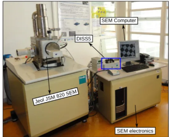
experiments have been realized. Fig. 4 shows the
Jeol JSM 820 SEM
SEM electronics DISS5
SEM Computer
Figure 4. Experimental set-up architecture.
experimental set-up architecture used for this work. The SEM used is a Jeol JSM 820 tungsten gun SEM equipped with a conventional Everhart-Thornley SE detector. Its electron column is equipped with dif-ferent sets of electromagnetic lenses and an objective aperture strip containing 4 changeable apertures of different diameters. The magnification of the SEM varies from ×10 to ×100, 000 and the maximum allow-able electronic working distance is 50 mm. A beam control and image acquisition system, DISS5 (from point electron GmbH) has been interfaced with the microscope. It is mainly responsible for sending the scan parameters to SEM and to acquire the data com-ing from SE detector. Later this data is amplified, digitized and saved as an image in the computer to which the DISS5 is connected. All the autofocus ex-periments are performed in this computer using the SE images of size 512 × 512 pixels and are monitored using the developed special purpose graphical user
interface program. Besides, DISS5 provides a user
interface control for the device focus by linking the working distance with a range of focus steps i.e., each step corresponds to a specific working distance. For real experiments with the system, a model given by (22) has been obtained by approximating the curve using least squares fitting. This model will be used to compute the corresponding focus step for a working distance given by (21) to modify the device focus.
F = PC=6 j=1 pjWC−j if 1 < W < 50 586 if W ≥ 50 973 if W ≤ 1 (22)
where, pi=1...6 are the coefficients of the model and
F is the focus step of the SEM. As the acceleration voltage used to excite the electrons vary the focusing model, for each voltage used in this work, a corre-sponding model has been derived. However, for the experiments, the voltage is fixed for all the tests per-formed with a specific sample.
4.2 Validation of the Method
Initial test is performed to validate the performance of the proposed method. The acceleration voltage used
100 μm
Figure 5. Microscale calibration rig1
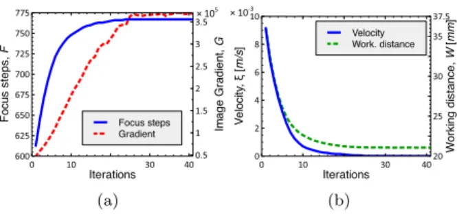
× 105 Focus steps Gradient Im a g e G ra d ie n t, G 0.5 1 1.5 2 2.5 3 3.5 F o c u s s te p s , F 600 625 650 675 700 725 750 775 Iterations 0 10 30 40 (a) × 10-3 Velocity Work. distance W o rk in g d is ta n c e , W [ m m ] 20 25 30 35 37.5 V e lo c it y, ξ [ m /s ] 0 2 4 6 8 10 Iterations 0 10 30 40 (b)
Figure 6. Validation of the method at a magnification
of ×300: Evolution of (a) focus step and image gradient (b) absolute velocity and working distance during the pro-posed process.
to generate the electron beam is 10 kV and has been fixed through all the experiments performed with this sample. The magnification used for this test is ×300 and the images are acquired with a raster scan speed of 720 nanoseconds/pixel, which provides a frame rate
of 2.2 frames per second. The sample for the
ex-periments is a microscale calibration rig containing chessboard patterns (Fig. 5). The brightness and the contrast are set to optimal values for the image acqui-sition process. The evolution of focus step and image gradient are shown in Fig. 6(a) and the variations of velocity and working distance are shown in Fig. 6(b). From the obtained results, it is evident that the veloc-ity decreases to zero when the image gradient reaches its maximum, which points out that the best focus has been accomplished successfully.
4.3 Validation under Different Conditions
Different sets of experiments have been conducted to validate the proposed method at various experimental conditions that include the variation in scan speed and magnification. Normally with SEM, usage of higher scan speeds or increasing magnification degrade the useful image information by increasing the level of random noise [16], which slightly affects the image gradient. However, any such influence can be read-ily compensated by the closed-loop control scheme. Apart from that, the performance of the method has also been evaluated by comparing it with an iterative search-based method [6]. It is a three fold technique that operates in three different iterations by varying the step size (distance between working distances) to search for the best focus position that provides the
1fabricated at FEMTO-ST Institute, France
Table 1. Autofocus results using optimal scan speed.
Mag. Obtained W (mm) Error (mm) proposed search manual proposed search 300 20.957 20.984 21.119 0.027 0.162 600 20.830 20.785 21.014 -0.045 0.184 900 20.830 20.864 20.811 0.034 -0.019 1200 21.114 21.037 21.012 -0.077 -0.102 RMSE 0.049 0.133
Table 2. Autofocus results using high scan speed.
Mag. Obtained W (mm) Error (mm) proposed search manual proposed search 300 20.891 20.953 20.817 0.062 -0.074 600 20.934 21.028 21.11 0.094 0.176 900 21.000 21.017 21.122 -0.070 0.122 1200 20.875 20.831 20.76 -0.044 -0.115 RMSE 0.055 0.127
maximum image sharpness. A normalized variance sharpness function has been used with this method. For the experiments, the step sizes used are 50, 5 and 1, respectively in each iteration. In both the cases i.e., for proposed and search-based methods, the optimum working distance estimated by a skilled human oper-ator has been used as the reference in computing the error.
As a pre-processing step, the images were filtered using a Gaussian filter of size 5 × 5 to reduce the level of noise. The magnification varies from ×300 to ×1200 with a step change of 300. The acceleration voltages used for the sample are 10 kV . Besides, all the experiments are performed in four different trials for any particular condition. The results shown are the average values of all these trials.
Table 1 and Table 2 summarize the obtained re-sults at different magnifications using scan speeds of 720 nanoseconds/pixel (optimal) and 180 nanosec-onds/pixel (high), respectively. From the results, it can be noticed that the accuracy of proposed method is better than search-based method under both con-ditions, with an improved average accuracy of 60% in comparison with the search-based method. This is mainly due to the fact that the proposed method is not affected by the lens hysteresis.
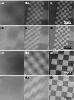
From analysis, the obtained results clearly show the efficiency and the repeatability of the proposed method of autofocus regardless of the sample sur-face as well as the experimental conditions. Some of the images acquired during different experiments are shown in the Fig. 7.
4.4 Discussion
The obtained experimental results show the accuracy and efficiency of the proposed method in the case of various real world scenarios. Since the Jacobian is computed analytically, the autofocus procedure is more robust w.r.t. the alternative methods (i.e. nu-merical computation of Jacobian or approximating the sharpness function to a simple function). Since the sum of squared norm of gradient has been consid-ered as a global sharpness function to be optimized by a closed loop control law, the efficiency of the method
The Journal’s name 15 µm 50 µm 50 µm 15 µm (a) (b) (c) (d) (e) (f) (g) (h) (i) (j) (k) (l)
Figure 7. Screenshots obtained during the autofocus
pro-cess: (a) to (c) with optimal scan speed at ×300 (d) to (f) with high scan speed at ×300 (g) to (i) with optimal scan speed at ×900 (j) to (l) with high scan speed at ×900. Last column depict the in-focus images.
will not be affected by changing the sample or the magnification of the SEM.
However, there are few limitations where the per-formance of the method could be affected. It should be mentioned that in our experiments the sample is flat. If the sample is far from perpendicular to the vision sensor, there is a risk that the sharpness func-tion could feature multiple optimum. Generally in a SEM, the support of sample can be set to be perpen-dicular to the electron gun by the SEM software. In this case, the tilt is normally smaller than the field of view, keeping the sample in-focus when the autofocus procedure achieve the optimization. Next, similar to the other autofocus techniques (using any imaging de-vice), the proposed method also requires the objects with sufficient texture information.
5 Conclusions
In this paper, an efficient and robust closed-loop control scheme has been proposed for a full scale autofocusing of SEM. The image gradient informa-tion is considered as the sharpness score in designing the vision-based control law. The optimum value of focus i.e., the maximum image sharpness has been
obtained by updating the device working distance
iteratively. The method has been validated on
different experimental conditions. Different from
other SEM autofocusing techniques, the derivative of the cost function is computed analytically, which makes the algorithm robust. Since the designed cost function reduces exponentially, the proposed method quickly converges to the optimal value.
References
[1] B.E. Kratochvil, L. Dong, B.J. Nelson, The In-ternational Journal of Robotics Research 28, 498 (2009)
[2] L. Cui, E. Marchand, International Journal of Optomechatronics 9, 151 (2015)
[3] Y. Sun, S. Duthaler, B. Nelson, in IEEE/RSJ Int. Conf. on Intelligent Robots and Systems (IROS) (2005), pp. 70–76
[4] M. Rudnaya, R. Mattheij, J. Maubach, Journal of microscopy 240, 38 (2010)
[5] S.J. Erasmus, K.C.A. Smith, Journal of Mi-croscopy 127, 185 (1982)
[6] C.F. Batten, Master’s thesis, Citeseer (2000) [7] M. Rudnaya, R. Mattheij, J. Maubach,
Mi-croscopy and Microanalysis 15, 1108 (2009) [8] M. Rudnaya, W. Van den Broek, R. Doornbos,
R. Mattheij, J. Maubach, Ultramicroscopy 111, 1043 (2011)
[9] M. Rudnaya, H. Ter Morsche, J. Maubach, R. Mattheij, J. Mathematical Imaging and Vi-sion 44, 38 (2012)
[10] N. Marturi, B. Tamadazte, S. Dembélé, N. Piat, in IEEE/RSJ Int. Conf. on Intelligent Robots and Systems (2013), pp. 2677–2682
[11] F. Nicolls, G. de Jager, B. Sewell, Ultrami-croscopy 69, 25 (1997)
[12] S.K. Nayar, Y. Nakagawa, IEEE Transactions on Pattern analysis and machine intelligence, 16, 824 (1994)
[13] J. Ens, P. Lawrence, IEEE Transactions on Pat-tern Analysis and Machine Intelligence, 15, 97 (1993)
[14] N. Cornille, Ph.D. thesis, École des Mines d’Albi, France (2005)
[15] E. Marchand, C. Collewet, in IEEE/RSJ Int. Conf. on Intelligent Robots and Systems (2010), pp. 5687–5692
[16] N. Marturi, S. Dembélé, N. Piat, Scanning 36, 419 (2014)