O
pen
A
rchive
T
OULOUSE
A
rchive
O
uverte (
OATAO
)
OATAO is an open access repository that collects the work of Toulouse researchers and
makes it freely available over the web where possible.
This is an author-deposited version published in :
http://oatao.univ-toulouse.fr/
Eprints ID : 15294
The contribution was presented at EuroNoise 2015 :
http://www.euronoise2015.eu/index.html
To cite this version :
Guyot, Patrice and Pinquier, Julien Soundscape visualization: a
new approach based on automatic annotation and Samocharts. (2015) In: 10th
European Congress and Exposition on Noise Control Engineering (EuroNoise 2015),
31 May 2015 - 3 June 2015 (Maastricht, Netherlands).
Any correspondence concerning this service should be sent to the repository
administrator:
[email protected]
Soundscape visualization: a new approach
based on automatic annotation and Samocharts
Patrice Guyot, Julien Pinquier
SAMoVA team - IRIT
University of Toulouse - France.
Summary
The visualization of sounds facilitates their identification and classification. However, in the case of audio recording websites, the access to a sound is usually based on the metadata of the sounds, i.e. sources and recording conditions. As sonic environments, or soundscapes, are mostly composed of multiples sources, their compact description is an issue that makes difficult the choice of an item in a sound corpus. The time-component matrix chart, which is abbreviated as TM-chart, has been proposed recently as a tool to describe and compare sonic environments. However their process of creation is based on a subjective annotation that makes their creation time-consuming. In this paper, we present a new method for urban soundscape corpus visualization. In the context of the CIESS project, we propose Samochart: an extension of the TM-chart that is based on sound detection algorithms. We describe three original algorithms that allow the detection of alarms, footsteps, and motors. Samocharts can be computed from the results of these algorithms. This process is applied to a concrete case study: 20 urban recordings of 5 minutes each, from different situations (places and time). An application case shows that Samocharts allow an identification of different situations. Finally, the whole method provides a low-cost tool for soundscape visualization that can easily be applied to the management and use of a sound corpus.
1.
Introduction
The visualization of sounds has always been a source of questioning. If the composer Olivier Messiaen, known as synesthetes, was able to perceive colors when he heard certain musical chords, the transla-tion of sound to image is generally not easy to for-malize. In the case of ethnomusicological studies for instance, transcriptions have traditionally been dis-tinguished between descriptive and prescriptive nota-tions according to their aims: the former are intended for analysis purpose, and the latter to reproduce the music [1]. This illustrates the difficulty to find an rep-resentation adapted to the needs of the users.
In the framework of environmental recordings, or soundscapes as introduced by Murray Schaffer, the issue of representation has been addressed since the 1970s [2]. If some works have been done in the focus of designing soundscapes (see [3] for interesting articles on this topic), one objective of soundscape represen-tations is to analyze and compare them.
When looking at the websites that propose brows-ing and downloadbrows-ing of field recordbrows-ings, the
display-(c) European Acoustics Association
ing of the sounds is usually based on a time/energy representation which can be slightly informative [4]. It seems indeed difficult to choose a sound from its waveform without hearing it. On websites such as freesound1
, textual metadata add a relevant informa-tion but remains generally insufficient to get an idea of what sounds compose the soundscape.
Through the CIESS project2
, we investigate the field of soundscape analysis and representation. Per-ception studies lead us to identify some sound events that seem characteristic of modern urban sound-scapes [5]. We assume that a representation based on this sound events can be efficient to represent a sound corpus.
Beside temporal representation, we decided to focus on illustrations that could globally display the pres-ence or abspres-ence of these sound events. The TM-chart representation provides us an efficient tool to repre-sent these recordings [6]. However, the costly human annotation makes it difficult to use in the context of a big corpus. In the regard of the growing improve-ment of automatic sound detection, we proposed a new framework of representation, inspired by
TM-1
https://www.freesound.org/
2
charts, that we call Samocharts [4]. Unlike TM-charts, Samocharts can be based on automatic detection algo-rithms, that makes their use possible without human annotation.
In this paper, we present a new approach for sound-scape visualization based on automatic event detec-tion algorithms. Secdetec-tion 2 introduces some relative works in this domain. Section 3, 4, and 5 describe our algorithms of sound detection to obtain confidence values, respectively on alarms, footsteps and motors. Section 6 presents an application case through the ur-ban recordings of the CIESS project.
2.
Relative works
2.1. Soundscape visualization
Soundscapes are usually materialized as quite long recordings, as its relative concepts focus significantly on the relationship with time. For instance, the du-ration of our recordings from the CIESS project are usually about 5 minutes. Longer observation record-ings have also been made in the context of acoustical ecology. For example, a recent study reports the vi-sualization of temporal change in soundscape power over a 4-year period [7], and revealed discrete patterns such as changes in the time of the occurrence of dawn and dusk choruses.
With long recordings, the traditional tools of au-dio representation, based on the temporal evolution of the signal, are slightly informative [4]. For exam-ple, urban recordings are too noisy to make appear semantic information from a waveform or a spectro-gram. However, these recordings are usually composed of the same kind of sound events, for instance vehi-cles, voices or birds. This fact provides an interesting entry point to alternative representations of sounds.
A new paradigm has been introduced in 2008 by Hiramatsu and al [6]. The time-component matrix chart, which is abbreviated as TM-chart, allows de-scribing and comparing sonic environments. It is a matrix that can be easily visualized as a figure to anal-yse and rapidly compare sonic environments. From a set of predetermined sound events, TM-charts provide a SoundSource×Soundlevel information for each tar-get sound. It shows the percentage of time of the sound source audibility and the percentage of time of its level range. However, their production process rely on the identification of the predominant sound at each time, which can be very costly in time. Thus, the TM-charts seem quite difficult to use on a big data set.
In a previous paper, we introduced Samocharts, a new approach inspired by charts [4]. As the TM-charts, the Samocharts are matrices that represent the percentage time of sound sources. Moreover, they can be computed from confidence values of sound detec-tion algorithms.
2.2. Audio event detection
Automatic annotation of audio recordings made sig-nificant progress these last years. These developments can be observed in the field of human voice with au-tomatic transcription, and emerge in the field of mu-sic with some applications like Shazam3
. From these observations, we shall assume that the detection of sound events in field recordings will become reliable in coming years.
Yet, various methods have been proposed on Au-dio Event Detection (AED) from auAu-dio files that have been recorded in real life. These works can be divided in two categories. The first one aims at detecting a large set of sounds in various contexts. These ap-proaches generally use machine learning techniques to automatically model a set of sounds from the evo-lution of acoustic features [8]. For example, the detec-tion of 61 sound events, such as bus door, footsteps or applause, has been reported in [9]. In this work the author model each sound class by an Hidden Markov Model (HMM) with 3 states, and Mel-Frequency Cep-stral Coefficients (MFCC) features.
A second category of methods aims at detecting specific sound events. These works are built up priv-ileging accuracy over the number of sounds that can be detected. They generally rely on a specific model-ing of the target sound that is based on acoustic ob-servations. For example, some studies propose to de-tect gunshots [10], water sounds [11], or alarms sounds [12, 13].
In this last reference, the authors compare the re-sults of alarm sounds detection with the two kinds of method mentioned. They show that a specific and simple approach can be more efficient that blind ma-chine learning techniques.
Moreover, due to numerous overlapping sound events, the urban sound recordings of our project are very noisy. In this context, the machine learning ap-proach seems currently inefficient. Thus, we choose to focus on particular sounds that slightly emerge from the noisy background and try to formalize the reasons of this emergence. Therefore, we built up ad hoc algo-rithms to detect these sounds. In the following parts, we will present our methods to detect alarms (such as car-horns), footsteps and motors.
3.
Alarm detection
3.1. Overview
Alarms are emblematic of urban soundscapes. They produce a sound event that convey urgent information or prevent efficiently a danger. In this regard, alarms such as car horns, sirens, and bicycle bell are usually built up to be easily audible and clearly identifiable.
3
Thus, humans seem able to identify a particular sound as an alarm even when they have never heard it before. However, the distinctive characteristics of alarm sounds are not formally defined. We suppose in the following work these sounds include acoustic invariants.
3.2. Method
In the CIESS corpus, we focused on three kinds of sound alarms: car horn, bus horn, and bicycle bell. Based on the observation of these sounds, we notice different acoustical properties that can be considered as invariants of alarm sounds. Our detection of these sounds is based on the following properties:
• duration longer than half a second,
• frequential stability over time (spectral lines), • medium and high frequencies preferred.
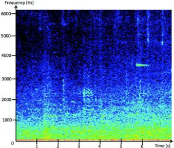
Moreover, the different kinds of alarms seen in the CIESS project show different distribution on spec-tral lines. Car horns are generally highly harmonic sounds. Bicycle bells in our corpus show one spectral line around 4000 Hz. Buses of the city of Toulouse show a particular horn with a spectral line around 1200 Hz. Figure 1 represent a spectrogram on which we can see two examples of these sounds.
Figure 1. Spectrogram of an urban soundscape extract from the CIESS project. Spectral lines from alarm sounds appear around 2 seconds at 1200 Hz, and at 6 seconds at 3800 Hz. The first sound is produced by a bus of the city of Toulouse and the second one by a bicycle.
Our method for alarm sound detection is based on the following steps: high-pass filtering, computation of a spectrogram, selection of spectral lines and iden-tification or reject of the founded candidates.
3.2.1. High-pass filtering
As alarm sounds are generally higher than 1000 Hz, we use a high-pass filter to suppress low frequencies and avoid potential false alarms. We use a high-pass digital Butterworth filter at order 10 with a cut fre-quency of 1500 Hz.
3.2.2. Computation of a spectrogram
We compute a spectrogram on the sound signal with a Fast Fourier Transform algorithm. As we look for a good frequency resolution, we compute each spectrum on windows of 120 milliseconds (2048 samples) with an overlapping of 75%.
3.2.3. Selection of spectral lines
The next step is to extract spectral lines from the spectrogram. We focus on small time/frequency rect-angles of 0.4 second width that are extracted from the spectrogram. We assume this duration is the minimal duration of an alarm sound.
On each rectangle, we compute temporal mean for each frequency. Each mean is afterwards compared with its neighbors on a frequency band of 300 Hz. If the mean if 3 times higher than its neighborhood, we consider that the spectral line is detected. Each rectangle of the signal which contains spectral lines is then considered as a potential candidate.
3.2.4. Identification or reject of candidates
We use a simple algorithm based on our observations mentioned above to validate the candidate. This algo-rithm relies on conditions on the number of spectral lines and their frequencies. This validation step allows to reject a false candidate or to identify a rectangle as car-horn, bus alarm, or bicycle bell sound.
This identification is then converted into values be-tween 0 and 1.
4.
Footstep detection
4.1. Overview
As walking remains one of the main way of moving, lots of people still walk in our city. Depending on their movement, their body and their shoes, these persons produce various sounds.
The footstep sounds are characterized by regular impacts. In the following method, we analyze the sig-nal to detect regular impacts.
4.2. Method
4.2.1. Computation of a spectrogram
We compute a spectrogram on the sound signal with a Fast Fourier Transform algorithm. As we look for a good temporal resolution, we compute each spectrum on windows of 30 milliseconds (512 samples) without overlapping. From this spectrogram, we focus on fre-quency bins ranging between 300 and 4000 Hz.
4.2.2. Peak extraction
We extract peaks from frames whose energy content is 3 times superior to the mean of its temporal neigh-borhood (on 100 frames around). We obtain a list of attack times.
4.2.3. Rhythm spectrum
To compute a rhythm spectrum, we focus on windows of 5 seconds and consider the attacks detected. We compute the Fourier transform of this attack times, as shown in the following equation:
RS(f req) = N bAttacks X i=1 e−2∗j∗π∗f req∗time(i) (1)
Where RS is the rhythm spectrum, N bAttacks the number of attacks, and time(i) the time of the ith
attack. This equation is applied to frequencies varying between 0.2 and 10 Hz.
Thus, on a particular frequency, a significant value in the rhythm spectrum reflects recursive attacks at this frequency.
4.2.4. Tempogram computation
By computing a rhythm spectrum at each sliding win-dow of the signal and concatenating them, we obtain a matrix that we call tempogram [14]. Each frame of the tempogram is a rhythm spectrum.
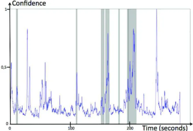
We extract the values of the tempogram that are superior to a masking threshold. We can see on figure 2 the orignal tempogram (2a) and tempogram supe-rior to a masking threshold (2b).
Then for each frame of the tempogram, we compute its sum divided by our decision threshold. We use 0.6 for the masking threshold and 250 for the decision threshold.
Figure 2. Tempograms and confidence values of footstep sound events on a 5 minutes urban soundscape extract from the CIESS project. The highlight parts correspond to the segment where we distinctly heard footsteps.
With setting values between 0 and 1, we obtain a confidence of repeated impacts at each time (2c).
5.
Motor detection
5.1. Overview
Motors of vehicles such as cars, mopeds, scooters and trucks, produce important noises that are characteris-tic of urban sound environment. In this step, we aim at detecting passages of motorized vehicles that emerge from the background sound.
5.2. Method
5.2.1. Computation of a spectrogram
We compute a spectrogram on the sound signal with a Fast Fourier Transform algorithm. We compute each spectrum on windows of 120 milliseconds (2048 sam-ples) with an overlap of 50%.
5.2.2. Spectral spread of low frequencies
We suppose that the motors sounds can be retrieved from their low frequencies. Thus, we extract from the spectrogram the frequency bins of the spectrogram ranging between 0 and 250 Hz. For each frame, we compute the spectral spread [15] on this frequency band.
5.2.3. Normalized local minimum
We compute the mean of these values on the whole signal. Local minima are then computed on group of frames of 6 second total duration, and divided by this mean.
Figure 3. Confidence values of motor sound events on a 5 minutes urban soundscape extract from the CIESS project. The highlight parts correspond to the segment where we distinctly heard the passage of a motor vehicle.
With setting values between 0 and 1, we obtain a probability of motors at each time.
6.
Application
6.1. Corpus
We use audio files from the CIESS project. From the city of Toulouse, at different place and time, we have recorded sound environment. There are three different schedules and situations:
• Non pedestrian street at 8 am, • Pedestrian street at noon, • Non pedestrian street at 9 pm.
The duration of each file is about 5 minutes. The recordings have been made with a Soundfiled SPS 200 microphone and a Tascam DR-680 recorder.
6.2. Sound event detection
The recordings are transformed in mono files with 16 kHz sampling rate. Our three detection algorithms are tuned on a recording of the corpus. Afterwards, we ran them on the full corpus and obtain time confidences for car horns, footsteps and motors for each file.
For each recording, our extraction methods give us temporal values of confidence on the presence of car-horns, footsteps, and motors. These values are inter-esting but cannot directly be interpreted as global and semantic information.
6.3. Visualization
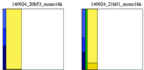
As defined in [4], we use the Samochart visualization to represent our corpus. The figure 4 represents all the Samocharts we plotted from our corpus. In these figures, we can see important duration of the signal (in white) where none of our target sounds were detected. A quick viewing shows differences in the recordings that are mainly relative to the presence of motors and footsteps. For instance, we notice that the last three recordings (in the direction of reading) exhibit a rel-ative larger part of footsteps. These recordings have indeed been made in pedestrian streets. Moreover, the other recordings, that have been recorded in different kind of streets, show a presence of motors more or less important. This could reflect different intensity of traffic according to different streets.
A zoom on the Samochart from the recordings lets appear the alarms (horns) sounds. Indeed, as horns sounds are usually very short events, the cumulative duration of these sounds can be very brief in com-parison of the duration of the whole signal. We can see on figure 5 two Samocharts, the first one with no car horn detected and the second one with car horn sounds.
7.
Conclusions and perspectives
In this paper, we presented methods to detect au-tomatically particular sound events in sound record-ings and to plot them with a new paradigm, the Samocharts.
Figure 4. Samocharts of recordings of the CIESS project. Each recording is represented by a square showing the percentage of time of presence of sound events. On each sound event, the confidence of the detection algorithm is shown by shades of colors.
Figure 5. Zoom on Samocharts of two recordings of the CIESS project.
7.1. Sound detection algorithms
The sound detection algorithms provide time values of confidence for the following sound events: car horns, footsteps and motors. Overall the algorithms seem to produce interesting results. However, they could be significantly improved with more annotated data. In-deed, the methods have been set up on a single anno-tated file, and could be tuned to a larger set on hetero-geneous files. Moreover, a greater number of manually annotated recordings could make possible to obtain a test data set and objective results of our algorithms. In this regard, our algorithms could be compared to state-of-the-art methods in order to choose the best approach. Some improvements could also be consid-ered, based for instance on the use of the Doppler effect in the motors sounds or the onset of the alarm sounds.
Furthermore, other methods and target sound events, such as voice, could also be added to our pack-age. After obtaining a stable version of our whole method, we should also consider saving computation time by pooling common processing, as the Fourier transform.
7.2. Browsing a sound corpus
The Samocharts based on automatic annotation al-gorithms provide an efficient way to browse a corpus of soundscapes. The whole method allows a fast com-parison of recordings. It seems to make possible the identification of particular situations, such as
pedes-trian streets. However, some experiments should be conducted to validate this concept.
Beside the zoom function, some improvements could be considered in our online displaying to facili-tate the browsing. For example, we could add research and sort functions based on sound events.
Elsewhere, it shall be mentioned that our approach describes a recording by the sum of its sound events, but does not take into consideration a more global perception of the Soundscapes (for example, we could consider a globally frightening recording). The con-cepts and methods needed to recognize such global feeling and display them should give us some works for coming years.
Acknowledgement
This work is supported by a grant from Agence Nationale de la Recherche with reference ANR-12-CORP-0013, within the CIESS project.
References
[1] Seeger, C. (1958). Prescriptive and descriptive music-writing. Musical Quarterly, 184-195.
[2] Schafer, R. M. (1977). The tuning of the world. Alfred A. Knopf.om
[3] COST Action TD0804 - Soundscape of European Cities and Landscapes.
[4] Guyot, P., & Pinquier, J. (2015). Browsing sound-scapes. First International Conference on Technologies for Music Notation and Representation. TENOR. [5] Tardieu, J., Magnen, C., Colle-Quesada, M.-M,
Spanghero-Gaillard, N., Gaillard, P., 2015. A method to collect representative samples of urban soundscapes. Euronoise 2015, 31 May - 3 June, Maastricht. [6] Hiramatsu, K., Matsui, T., Furukawa, S., and
Uchiyama, I., (2008). The physcial expression of
soundscape: An investigation by means of time com-ponent matrix chart, in INTERNOISE and NOISE-CON Congress and Conference Proceedings, vol. 2008, no. 5.Institute of Noise Control Engineering, 2008, pp. 4231-4236.
[7] Gage, S. H., & Axel, A. C. (2014). Visualization of temporal change in soundscape power of a Michigan lake habitat over a 4-year period. Ecological Informat-ics, 21, 100-109.
[8] Giannoulis, D., Benetos, E., Stowell, D., Rossignol, M., Lagrange, M., & Plumbley, M. D. (2013). Detec-tion and classificaDetec-tion of acoustic scenes and events: an IEEE AASP challenge. In Applications of Signal Processing to Audio and Acoustics (WASPAA), 2013 IEEE Workshop on (pp. 1-4).
[9] Mesaros, A., Heittola, T., Eronen, A., & Virtanen, T. (2010). Acoustic event detection in real life recordings. In 18th European Signal Processing Conference (pp. 1267-1271).
[10] Clavel, C., Ehrette, T., & Richard, G. (2005). Events detection for an audio-based surveillance system. In Multimedia and Expo, 2005. ICME 2005. IEEE Inter-national Conference on (pp. 1306-1309).
[11] Guyot, P., Pinquier, J., & André-Obrecht, R. (2013). Water sound recognition based on physical models. In Acoustics, Speech and Signal Processing (ICASSP), 2013 IEEE International Conference on (pp. 793-797). [12] Lutfi, R. A., & Heo, I. (2012). Automated detection of alarm sounds. The Journal of the Acoustical Society of America, 132(2), EL125-EL128.
[13] Ellis, D. P. (2001). Detecting alarm sounds. In Con-sistent & Reliable Acoustic Cues for Sound Analy-sis: One-day Workshop: Aalborg, Denmark, Sunday, September 2nd, 2001 (pp. 59-62). Department of Elec-trical Engineering, Columbia University.
[14] Le Coz, M. (2014). Spectre de rythme et sources mul-tiples: au cœur des contenus ethnomusicologiques et sonores (Doctoral dissertation, Toulouse 1).
[15] Peeters, G. (2004). A large set of audio features for sound description (similarity and classification) in the CUIDADO project.