Deep Exploration of ɛ Eridani with Keck Ms-band Vortex Coronagraphy and Radial Velocities: Mass and Orbital Parameters of the Giant Exoplanet

Deep Exploration of

ò Eridani with Keck Ms-band Vortex Coronagraphy and Radial

Velocities: Mass and Orbital Parameters of the Giant Exoplanet

Dimitri Mawet1,2 , Lea Hirsch3,4 , Eve J. Lee5 , Jean-Baptiste Ruffio6 , Michael Bottom2 , Benjamin J. Fulton7 , Olivier Absil8,20 , Charles Beichman2,9,10, Brendan Bowler11 , Marta Bryan1 , Elodie Choquet1,21 , David Ciardi7, Valentin Christiaens8,12,13, Denis Defrère8 , Carlos Alberto Gomez Gonzalez14 , Andrew W. Howard1 , Elsa Huby15, Howard Isaacson4 , Rebecca Jensen-Clem4,22 , Molly Kosiarek16,23 , Geoff Marcy4 , Tiffany Meshkat17 , Erik Petigura1 ,

Maddalena Reggiani8 , Garreth Ruane1,24 , Eugene Serabyn2, Evan Sinukoff18 , Ji Wang1 , Lauren Weiss19 , and Marie Ygouf17

1

Department of Astronomy, California Institute of Technology, Pasadena, CA 91125, USA;dmawet@astro.caltech.edu 2

Jet Propulsion Laboratory, California Institute of Technology, Pasadena, CA 91109, USA

3

Kavli Institute for Particle Astrophysics and Cosmology, Stanford University, Stanford, CA 94305, USA

4

University of California, Berkeley, 510 Campbell Hall, Astronomy Department, Berkeley, CA 94720, USA

5

TAPIR, Walter Burke Institute for Theoretical Physics, Mailcode 350-17, Caltech, Pasadena, CA 91125, USA

6

Kavli Institute for Particle Astrophysics and Cosmology, Stanford University, Stanford, CA 94305, USA

7

NASA Exoplanet Science Institute, Caltech/IPAC-NExScI, 1200 East California Boulevard, Pasadena, CA 91125, USA

8_{Space sciences, Technologies & Astrophysics Research(STAR) Institute, Université de Liège, Allée du Six Août 19c, B-4000 Sart Tilman, Belgium} 9

Division of Physics, Mathematics, and Astronomy, California Institute of Technology, Pasadena, CA 91125, USA

10

NASA Exoplanet Science Institute, 770 S. Wilson Avenue, Pasadena, CA 911225, USA

11

McDonald Observatory and the University of Texas at Austin, Department of Astronomy, 2515 Speedway, Stop C1400, Austin, TX 78712, USA

12

Departamento de Astronomía, Universidad de Chile, Casilla 36-D, Santiago, Chile

13

Millennium Nucleus“Protoplanetary Disks in ALMA Early Science,” Chile

14

Université Grenoble Alpes, IPAG, F-38000 Grenoble, France

15

LESIA, Observatoire de Paris, Meudon, France

16

University of California, Santa Cruz; Department of Astronomy and Astrophysics, Santa Cruz, CA 95064, USA

17_{IPAC, California Institute of Technology, M/C 100-22, 770 S. Wilson Ave, Pasadena, CA 91125, USA} 18

Institute for Astronomy, University of Hawai’i at Manoa, Honolulu, HI 96822, USA

19_{Institut de Recherche sur les Exoplanètes, Dèpartement de Physique, Universitè de Montrèal, C.P. 6128, Succ. Centre-ville, Montréal, QC H3C 3J7, Canada}

Received 2018 May 1; revised 2018 October 16; accepted 2018 October 29; published 2019 January 3

Abstract

We present the most sensitive direct imaging and radial velocity(RV) exploration of ò Eridani to date. ò Eridani is an adolescent planetary system, reminiscent of the early solar system. It is surrounded by a prominent and complex debris disk that is likely stirred by one or several gas giant exoplanets. The discovery of the RV signature of a giant exoplanet was announced 15 yr ago, but has met with scrutiny due to possible confusion with stellar noise. We confirm the planet with a new compilation and analysis of precise RV data spanning 30 yr, and combine it with upper limits from our direct imaging search, the most sensitive ever performed. The deep images were taken in the Ms band(4.7 μm) with the vortex coronagraph recently installed in W.M. Keck Observatory’s infrared camera NIRC2, which opens a sensitive window for planet searches around nearby adolescent systems. The RV data and direct imaging upper limit maps were combined in an innovative joint Bayesian analysis, providing new constraints on the mass and orbital parameters of the elusive planet.ò Eridani b has a mass of 0.78-+0.120.38MJupand is

orbitingò Eridani at about 3.48±0.02 au with a period of 7.37±0.07 yr. The eccentricity of ò Eridani b’s orbit is 0.07 0.05

0.06

-+ _{, an order of magnitude smaller than early estimates and consistent with a circular orbit. We discuss our}

findings from the standpoint of planet–disk interactions and prospects for future detection and characterization with the James Webb Space Telescope.

Key words: planet–disk interactions – planets and satellites: dynamical evolution and stability – planets and satellites: gaseous planets– stars: planetary systems – techniques: high angular resolution – techniques: radial velocities

Supporting material: machine-readable tables

1. Introduction

ò Eridani is an adolescent (200–800 Myr) (Fuhrmann2004; Mamajek & Hillenbrand2008) K2V dwarf star (Table1). At a

distance of 3.2 pc,ò Eridani is the tenth closest star to the Sun, which makes it a particularly attractive target for deep planet searches. Its age, spectral type, distance, and consequent apparent brightness (V=3.73 mag) make it a benchmark system, as well as an excellent analog for the early phases of the solar system’s evolution. ò Eridani hosts a prominent, complex debris disk, and a putative Jupiter-like planet. © 2019. The American Astronomical Society. All rights reserved.

* _{Based on observations obtained at the W. M. Keck Observatory, which is}

operated jointly by the University of California and the California Institute of Technology. Keck time was granted for this project by Caltech, the University of Hawai’i, the University of California, and NASA.

20

F.R.S.-FNRS Research Associate.

21

Hubble Postdoctoral Fellow.

22

Miller Fellow.

23

NSF Graduate Research Fellow.

24

1.1.ò Eridani’s Debris Disk

The disk was first detected by the Infrared Astronomical Satellite (Aumann 1985) and later on by the Infrared Space

Observatory(Walker & Heinrichsen2000). It was first imaged

by the Submillimetre Common-User Bolometer Array (SCUBA) at the James Clerk Maxwell Telescope by Greaves et al.(1998). ò Eridani is one of the “fabulous four” Vega-like

debris disks and shows more than 1 Jy of far-infrared (FIR) excess over the stellar photosphere at 60–200 μm and a lower significance excess at 25 μm (Aumann1985). Using the Spitzer

Space Telescope and the Caltech Submillimeter Observatory (CSO) to trace ò Eridani’s spectral energy distribution (SED) from 3.5 to 350μm, the model presented in Backman et al. (2009) paints a complex picture. ò Eridani’s debris disk is

composed of a main ring at 35–90 au, and a set of two narrow inner dust belts inside the cavity delineated by the outer ring: one belt with a color temperature T;55 K at approximately 20 au, and another belt with a color temperature T;120 K at approximately 3 au (Backman et al.2009). The authors argue

that, to maintain the three-belt system around ò Eridani, three shepherding planets are necessary.

Using Herschel at 70, 160, 250, 350, and 500μm, Greaves et al.(2014) refined the position and the width of the outer belt

to be 54–68 au, but only resolved one of the inner belts at 12–16 au. More recently, Chavez-Dagostino et al. (2016) used

the Large Millimetre Telescope Alfonso Serrano (LMT) at 1.1 mm and resolved the outer belt at a separation of 64 au. Emission is detected at the location of the star in excess of the photosphere. The angular resolution of the 1.1 mm map, however, is not sufficient to resolve the inner two warm belts of Backman et al. (2009). MacGregor et al. (2015) used the

Submillimeter Array (SMA) at 1.3 mm and the Australia Telescope Compact Array(ATCA) at 7 mm to resolve the outer ring and measure its width (measurement now superseded by ALMA, see below). The data at both mm wavelengths show excess emission, which the authors attribute to ionized plasma from a stellar corona or chromosphere.

Su et al.(2017) recently presented 35 μm images of ò Eridani

obtained with the Stratospheric Observatory for Infrared Astronomy (SOFIA). The inner disk system is marginally resolved within 25 au. Combining the 15–38 μm excess spectrum with Spitzer data, Su et al. (2017) find that the

presence of in situ dust-producing planetesimal belt(s) is the most likely source of the infrared excess emission in the inner 25 au region. However, the SOFIA data are not constraining enough to distinguish one broad inner disk from two narrow belts.

Booth et al. (2017) used the Atacama Large Millimeter/

submillimeter Array (ALMA) to image the northern arc of the outer ring at high angular resolution(beam size <2″). The 1.34 mm continuum image has a low signal-to-noise ratio (S/N) but is well-resolved, with the outer ring extending from 62.6 to 75.9 au. The fractional outer disk width is comparable to that of the solar system’s Kuiper Belt and makes it one of the narrowest debris disks known, with a width of just ;12 au. The outer ring inclination is measured to be i=34°±2°, consistent with all previous estimates using lower-resolution submm facilities (Greaves et al. 1998, 2005; Backman et al.

2009). No significant emission is detected between ∼20 and

∼60 au (see Booth et al. (2017), their Figure 5), suggesting a

large clearing between the inner belt(s) within 20 au and the outer belt outward of 60 au. Booth et al.(2017) find tentative

evidence for clumps in the ring, and claim that the inner and outer edges are defined by resonances with a planet at a semimajor axis of 48 au. The authors also confirm the previous detection of unresolved mm emission at the location of the star that is above the level of the photosphere and attribute this excess to stellar chromospheric emission, as suggested by MacGregor et al. (2015). However, the chromospheric

emission cannot reproduce the infrared excess seen by Spitzer and SOFIA.

Finally, recent 11μm observations with the Large Binocular Telescope Interferometer (LBTI) suggest that warm dust is present within∼500 mas (or 1.6 au) from ò Eridani (Ertel et al.

2018). The trend of the detected signal with respect to the

stellocentric distance also indicates that the bulk of the emission comes from the outer part of the LBTIfield of view, and hence is likely associated with the dust belt(s) responsible for the 15–38 μm emission detected by Spitzer and SOFIA.

1.2. ò Eridani’s Putative Planet

Hatzes et al. (2000) demonstrated that the most likely

explanation for the observed decade-long radial velocity(RV) variations was the presence of a;1.5 MJ giant planet with a

period P=6.9 yr (;3 au orbit) and a high eccentricity (e=0.6). While most of the exoplanet community seems to have acknowledged the existence ofò Eridani b, there is still a possibility that the measured RV variations are due to stellar activity cycles (Anglada-Escudé & Butler 2012; Zechmeister et al. 2013). Backman et al. (2009) rightly noted that a giant

planet with this orbit would quickly clear the inner region not only of dust particles but also the parent planetesimal belt needed to resupply them, inconsistent with their observations.

1.3. This Paper

In this paper, we present the deepest direct imaging reconnaissance ofò Eridani to date, a compilation of precision RV measurements spanning 30 years, and an innovative joint Bayesian analysis combining both planet detection methods. Our results place the tightest constraints yet on the planetary mass and orbital parameters for this intriguing planetary system. The paper is organized as follows: Section2describes the RV observations and data analysis, Section3describes the high-contrast imaging observations and post-processing, Section4presents our nondetection and robust detection limits from direct imaging, additional tests on the RV data, and our joint analysis of both data sets. In Section 5, we discuss our findings, the consequences of the new planet parameters on

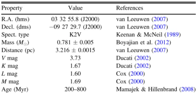
Table 1 Properties ofò Eridani

Property Value References

R.A.(hms) 03 32 55.8(J2000) van Leeuwen(2007) Decl.(dms) −09 27 29.7 (J2000) van Leeuwen(2007) Spect. type K2V Keenan & McNeil(1989) Mass(Me) 0.781±0.005 Boyajian et al.(2012) Distance(pc) 3.216±0.0015 van Leeuwen(2007)

V mag 3.73 Ducati(2002)

K mag 1.67 Ducati(2002)

L mag 1.60 Cox(2000)

M mag 1.69 Cox(2000)

planet–disk interactions, and prospects for detection with the James Webb Space Telescope, before concluding in Section6.

2. Doppler Spectroscopy

In this section, we present our new compilation and analysis of Doppler velocimetry data of ò Eridani spanning 30 yr.

2.1. RV Observations

ò Eridani has been included in planet search programs at both Keck Observatory using the HIRES Spectrometer (Howard et al. 2010) and at Lick Observatory using the Automated

Planet Finder (APF) and Levy Spectrometer. ò Eridani was observed on 206 separate nights with HIRES and the APF, over the past 7 yr.

Keck/HIRES (Vogt et al. 1994) RV observations were

obtained starting in 2010, using the standard iodine cell configuration of the California Planet Survey (CPS) (Howard et al.2010). During the subsequent 7 yr, 91 observations were

taken through the B5 or C2 deckers (0 87×3 5, and 0 87×14″, respectively), yielding a spectral resolution of R≈55,000 for each observation. Each measurement was taken through a cell of gaseous molecular iodine heated to 50°C, which imprints a dense forest of iodine absorption lines onto the stellar spectrum in the spectral region of 5000–6200 Å. This iodine spectrum was used for wavelength calibration and as a PSF reference. Each RV exposure was timed to yield a per-pixel S/N of 200 at 550 nm, with typical exposure times of only a few seconds due to the brightness of the target. An iodine-free template spectrum was obtained using the B3 decker (0 57×14″, R≈72,000) on 2010 August 30.

RV observations using the APF and Levy Spectrograph (Radovan et al.2014; Vogt et al.2014) were taken starting in

late 2013. The APF is a 2.4 m telescope dedicated to performing RV detection and follow-up of planets and planet candidates, also using the iodine cell method of wavelength calibration. APF data onò Eridani were primarily taken through the W decker (1″×3″), with a spectral resolution of R≈ 110,000. Exposures were typically between 10 and 50 s long, yielding S/N per-pixel of 140. The typical observing strategy at the APF was to take three consecutive exposures and then bin them to average over short-term fluctuations from stellar oscillations. On some nights, more than one triple-exposure was taken. These were binned on a nightly timescale. An iodine-free template consisting of five consecutive exposures was obtained on 2014 February 17 using the N decker (0 5×8″) with resolution R≈150,000. Both the APF and HIRES RVs were calibrated to the solar system barycenter and corrected for the changing perspective caused by the high proper motion ofò Eridani.

In addition to the new HIRES and APF RV data, we incorporate previously published data from several telescopes into this study. High-precision RV observations of ò Eridani were taken with the Hamilton spectrograph at Lick Observatory starting in 1987, as part of the Lick Planet Search program. They were published in the catalog of Fischer et al. (2014),

along with details of the instrumental setup and reduction procedure.

The Coudé Echelle Spectrograph at La Silla Observatory was used, first with the Long Camera (LC) on the 1.4 m telescope from 1992 to 1998, then with the Very Long Camera (VLC) on the 3.6 m telescope from 1998 to 2006, to collect

additional RV data onò Eridani. RV data were also collected using the HARPS spectrograph, also on the 3.6 m telescope at La Silla Observatory, during 2004–2008. Together, these data sets were published in Zechmeister et al.(2013).

2.2. RV Data Analysis

All new spectroscopic observations from Keck/HIRES and APF/Levy were reduced using the standard CPS pipeline (Howard et al.2010). The iodine-free template spectrum was

deconvolved with the instrumental PSF and used to forward model each observation’s relative RV. The iodine lines imprinted on the stellar spectrum by the iodine cell were used as a stable wavelength calibration, and the instrumental PSF was modeled as the sum of several Gaussians (Butler et al.

1996). Per the standard CPS RV pipeline, each spectrum was

divided into approximately 700 spectral“chunks” for which the RV was individually calculated. The final RV and internal precision were calculated as the weighted average of each of these chunks. Chunks with RVs that are more consistent across observations are given higher weight. Those chunks with a larger scatter are given a lower weight. The RV observations from Keck/HIRES and APF/Levy are listed in Tables5and6, respectively. These data are not offset-subtracted to account for different zero-points, and the uncertainties reported in the tables reflect the weighted standard deviations of the chunk-by-chunk RVs and do not include systematic uncertainty such as jitter.

In combination among HIRES, the APF, and the other instruments incorporated, a total of 458 high-precision RV observations have been taken, over an unprecedented time baseline of 30 yr. We note that the literature RV data included in this study were analyzed using a separate RV pipeline, which in some cases did not include a correction for the secular acceleration of the star. Secular acceleration is caused by the space motion of a star and depends on its proper motion and distance. For ò Eridani, we calculate a secular acceleration signal of 0.07 ms−1yr−1 (Zechmeister et al. 2009). This is

accounted for in the HIRES and APF data extraction, and most likely in the Lick pipeline, but is not included in the reduction for the CES and HARPS data. However, the amplitude of this effect is much smaller than the amplitude of RV variation observed in the RVs due to stellar activity and the planetary orbit. Because each of the CES and HARPS data sets cover less than 10 yr, we expect to see less than 1m s-1_{variation across}

each full data set. We tested running the analysis with and without applying these corrections. All of the resulting orbital parameters were consistent to within ∼0.1σ. We therefore neglect this correction in our RV analyses. From the combined RV data set, a clear periodicity of approximately 7 yr is evident, both by eye and in a periodogram of the RV data. We assess this periodicity in Section4.2.

ò Eridani’s youth results in significant stellar magnetic activity. Convection-induced motions on the stellar surface cause slight variations in the spectral line profiles, leading to variations in the inferred RV that do not reflect motion caused by a planetary companion. As a result, stellar magnetic activity may mimic the RV signal of an orbiting planet, resulting in false positives. We therefore extract SHK values from each of

the HIRES and APF spectra taken for ò Eridani. SHK is a

measure of the excess emission at the cores of the CaIIH and K lines due to chromospheric activity; it correlates with stellar magnetic activity, such as spots and faculae, which might have

effects on the RVs extracted from the spectra (Isaacson & Fischer 2010).

3. High-contrast Imaging

Here, we present our new deep, direct, high-contrast imaging observations and data analysis of ò Eridani using the Keck NIRC2 vortex coronagraph.

3.1. High-contrast Imaging Observations

We observedò Eridani over three consecutive nights in 2017 January (see Table 2). We used the vector vortex

coronagraph installed in NIRC2 (Serabyn et al. 2017), the

near-infrared camera and spectrograph behind the adaptive optics system of the 10 m Keck II telescope at W.M. Keck Observatory. The vortex coronagraph is a phase-mask coronagraph enabling high-contrast imaging at very small angles close to the diffraction limit of the 10 m Keck telescope at 4.67μm (;0 1). The starlight suppression capability of the vortex coronagraph is induced by a 4π radian phase ramp wrapping around the optical axis. When the coherent adaptively corrected point spread function (PSF) is centered on the vortex phase singularity, the on-axis starlight is redirected outside the geometric image of the telescope pupil formed downstream from the coronagraph, where it is blocked by means of an undersized diaphragm (the Lyot stop). The vector vortex coronagraph installed in NIRC2 was made from a circularly concentric subwavelength grating etched onto a synthetic diamond substrate (Annular Groove Phase Mask coronagraph or AGPM) (Mawet et al. 2005; Vargas Catalán et al.2016).

Median 0.5μm DIMM seeing conditions ranged from 0 52 to 0 97 (see Table 2). The adaptive optics system provided

excellent correction in the Ms-band([4.549, 4.790] μm) with a Strehl ratio of about 90%(NIRC2 quicklook estimate), similar to the image quality provided at shorter wavelengths by extreme adaptive optics systems such as the Gemini Planet Imager(GPI, Macintosh et al. 2014), SPHERE (Beuzit et al. 2008), and

SCExAO(Jovanovic et al.2015). The alignment of the star onto

the coronagraph center, a key to high contrast at small angles, was performed using the quadrant analysis of coronagraphic images for tip-tilt sensing(QACITS) (Huby et al.2015,2017).

The QACITS pointing control uses NIRC2 focal-plane corona-graphic science images in a closed feedback loop with the Keck adaptive optics tip-tilt mirror (Huby et al. 2017; Mawet et al. 2017; Serabyn et al. 2017). The typical low-frequency

centering accuracy provided by QACITS is;0.025λ/D rms, or ;2 mas rms.

All of our observations were performed in vertical angle mode, which forces the AO derotator to track the telescope pupil (following the elevation angle) instead of the sky, effectively allowing thefield to rotate with the parallactic angle, enabling angular differential imaging(ADI) (Marois et al.2006).

3.2. Image Post-processing

After correcting for bad pixels,flat-fielding, subtracting sky background frames using principal component analysis(PCA), and co-registering the images, we applied PCA(Soummer et al.

2012; Gomez Gonzalez et al.2017) to estimate and subtract the

post-coronagraphic residual stellar contribution from the images. We used the open-source Vortex Image Processing— VIP25—software package (Gomez Gonzalez et al.2017), and

applied PCA on the combined data from all three nights, totaling more than 5 hr of open shutter integration time (see Table2for details). We used a numerical mask 2λ/D in radius to occult the bright stellar residuals close to the vortex coronagraph inner working angle.

Thefinal image (Figure1) was obtained by pooling all three

nights together in a single data set totaling 624 frames. The PSF was reconstructed by using 120 principal components and projections on the 351×351 pixel frames excluding the central numerical mask (2λ/D in radius). This number of principal components was optimized to yield the best final contrast limits in the 1–5 au region of interest, optimally trading

Table 2

Observing log for NIRC2 Imaging Data

Properties Value Value Value

UT date(yyyy mm dd) 2017-01-09 2017-01-10 2017-01-11 UT start time(hh: mm:ss) 05:11:55 05:12:47 05:48:08 UT end time(hh: mm:ss) 09:14:11 09:31:09 08:36:14

Discr. Int. Time(s) 0.5 L L

Coadds 60 L L

Number of frames 210 260 154

Total integration time(s)

6300 7800 4620

Plate scale(mas/pix) 9.942(“narrow”) L L Total FoV r;5″ (vortex

mount)

L L

Filter Ms[4.549,

4.790] μm

L L

Coronagraph Vortex(AGPM) L L

Lyot stop Inscribed circle L L

0.5μm DIMM see-ing(″)

0.52 0.64 0.97

Par. angle start-end(°) −36–+52 −35–+55 −20–+46

Figure 1.Final reduced image ofò Eridani, using PCA, and 120 principal components in the PSF reconstruction. The scale is linear in analog to digital units(ADU).

25

off speckle noise and self-subtraction effects. Thefinal image (Figure 1) does not show any particular feature and is

consistent with whitened speckle noise. 4. Analysis

In this section, we present our nondetection and robust detection limits from direct imaging, additional tests on the RV data, as well as our joint analysis of both data sets.

4.1. Robust Detection Limits from Direct Imaging Following Mawet et al. (2014), we assume that ADI and

PCA post-processing whiten the residual noise in the final reduced image through two complementary mechanisms. First, PCA removes the correlated component of the noise by subtracting off the stellar contribution, revealing underlying independent noise processes such as background, photon Poisson noise, readout noise, and dark current. Second, the ADI frame combination provides additional whitening due to thefield rotation during the observing sequence and subsequent derotation, and by virtue of the central limit theorem, regardless of the underlying distribution of the noise (Marois et al.

2006, 2008). Henceforth, we assume Gaussian statistics to

describe the noise of our images. Our next task is to look for point sources, and if none are found, place meaningful upper limits. Whether or not point sources are found, we will use our data to constrain the planet mass posterior distribution as a function of projected separation.

For this task, we choose to convert flux levels into mass estimates using the COND evolutionary model (Baraffe et al.

2003) for the three ages considered in this work: 200, 400, and

800 Myr. The young age end of our bracket (200 Myr) is derived from a pure kinematic analysis(Fuhrmann2004). The

400 and 800 Myr estimates are from Mamajek & Hillenbrand (2008), who used chromospheric activities and spin as age

indicators.

As noted by Bowler(2016), the COND model is part of the

hot-start model family, which begins with arbitrarily large radii and oversimplified, idealized initial conditions. It ignores the effects of accretion and mass assembly. The COND model represents the most luminous—and thus optimistic—outcome. At the adolescent age range of ò Eridani, initial conditions of the formation of a Jupiter-mass gas giant have mostly been forgotten (Marley et al.2007; Fortney et al.2008) and have a

minor impact on mass estimates. Moreover, a very practical reason why COND was used is because it is the only model readily providing open-source tables extending into the low-mass regime 9<1 MJup) reached by our data (see Section5.1).

4.1.1. Direct Imaging Nondetection

Signal detection is a balancing act where one trades off the risk of false alarm with sensitivity. The signal detection thresholdτ is related to the risk of false alarm, or false positive fraction(FPF), as follows: p x H dx FPF FP TN FP

ò

where x is the intensity of the residual speckles in our images, p x H( ∣ 0) is the probability density function of x under the null

hypothesis H0, FP is the number of false positives, and TN is

the number of true negatives. Assuming Gaussian noise

statistics, the traditional τ=5σ threshold yields an FPF of 2.98×10−7.

Applying the τ=5σ threshold to the S/N map generated from our most sensitive reduction, which occurs for a number of principal components equal to 120, yields no detection, consistent with a null result. In other words,ò Eridani b is not detected in our deep imaging data to the 5σ threshold. To compute the S/N map, we used the annulus-wise approach outlined in Mawet et al.(2014), and implemented in the

open-source Python-based Vortex Imaging Pipeline(Gomez Gonzalez et al.2017). The noise in an annulus at radius r (units of λ/D) is

computed as the standard deviation of the n=2πr resolution elements at that radius. The algorithm throughput is computed using fake companion injection-recovery tests at every location in the image. This step is necessary to account for ADI self-subtraction effects. The result is shown in Figure2.

To quantify our sensitivity, also known as“completeness,” we use the true positive fraction(TPF), defined as

p x H dx TPF TP TP FN

ò

with p x H( ∣ 1), the probability density function of x under the

hypothesis H1—signal present, and where TP is the number of

true positives and FN the number of false negatives. For instance, a 95% sensitivity(or completeness) for a given signal I and detection thresholdτ means that 95% of the objects at the intensity level I will statistically be recovered from the data.

The sensitivity contours, or “performance maps” (Jensen-Clem et al. 2018) for a uniform threshold corresponding to

2.98×10−7 FPF are shown in Figure 4. The choice of threshold is assuming Gaussian noise statistics and accounts for small sample statistics as in Mawet et al.(2014). At the location

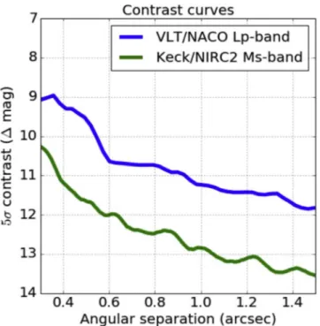
of the elusive RV exoplanet, the threshold corrected for small sample statistics converges to τ≈5σ. The corresponding traditional τ=5σ contrast curve at 50% completeness is shown in Figure3.

Figure 2. S/N map for our most sensitive reduction, using 120 principal components. We used the S/N map function implemented in open source package VIP(Gomez Gonzalez et al.2017). The method uses the annulus-wise approach presented in Mawet et al.(2014). No source is detected above 5σ. The green circle delineates the planet’s project separation at ;3.5 au.

4.1.2. Comparison to Previous Direct Imaging Results

Mizuki et al. (2016) presented an extensive direct imaging

compilation and data analysis for ò Eridani. The authors analyzed data from Subaru/HiCIAO, Gemini/NICI, and VLT/ NACO. Here, we focus on the deepest data set reported in Mizuki et al.(2016), which is the Lp-band NACO data from PI:

Quanz(Program ID: 090.C-0777(A)). This non-coronagraphic ADI sequence totals 146.3 minutes of integration time and about 67° of parallactic angle rotation. Mizuki et al. (2016)

report 5σ and 50% completeness mass sensitivities using the hot start COND evolutionary model that are>10 MJat 1 au for

all three ages considered here, i.e., 200, 400, and 800 Myr; at 2 au, they are ;2.5 MJ,;4 MJ, and;6.5 MJ, respectively; at

3 au, they are;2 MJ,;3 MJ, and;5 MJ, respectively.

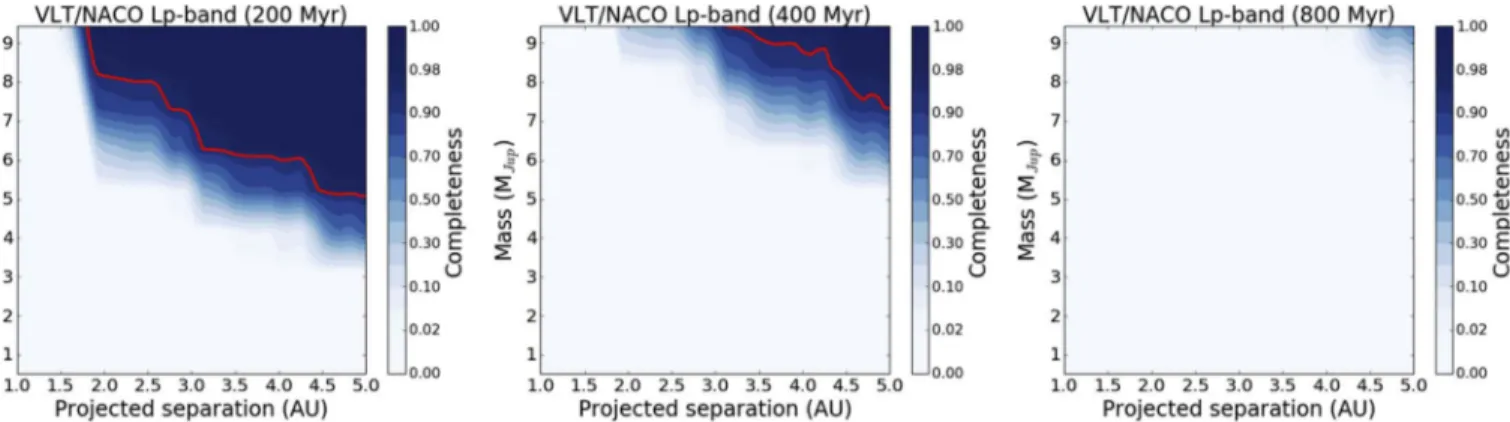
For consistency, we reprocessed the VLT/NACO data with the VIP package and computed completeness maps using the same standards as for our Keck/NIRC2 data. The results are shown in Figure 5. Our computed 5σ and 50% completeness mass sensitivities using the hot start COND evolutionary model for the VLT/NACO Lp-band data are >10 MJ at 1 au for all

three ages considered here, i.e., 200, 400, and 800 Myr; at 2 au, they are ;6.5 MJ at 200 Myr and >10 MJ at both 400 and

800 Myr; at 3 au, they are ;5.5 MJ, ;8 MJ, and >10 MJ,

respectively.

Our computed 5σ and 50% completeness results for the VLT/NACO Lp-band data are systematically worse than those presented in Mizuki et al. (2016). We note a discrepancy in

mass between the published results and our values, by a factor of two. We suggest that it may be the result of inaccurateflux loss calibrations in Mizuki et al. (2016), which is a common

occurrence with ADI data sets.

Wefind that our Ms-band Keck/NIRC2 coronagraphic data is about a factor of 5–10 more sensitive in mass, across the range of solar system scales probed in this work, than the previous best available data set. Our 5σ and 50% completeness

mass sensitivities using the hot start COND evolutionary model are ;3 MJ, ;4.5 MJ, and ;6.5 MJ at 1 au for all three ages

considered here, i.e., 200, 400, and 800 Myr, respectively; at 2 au, they are;1.5 MJ,;1.7 MJ, and;2.5 MJ, respectively; at

3 au, they are;0.8 MJ,;1.7 MJ, and;5 MJ, respectively.

These results demonstrate the power of ground-based Ms-band small-angle coronagraphic imaging for nearby adoles-cent systems. When giant exoplanets cool down to below 1000 K, the peak of their blackbody emission shifts to 3–5 μm mid-infrared wavelengths. Moreover, due to the t−5/4 depend-ence of bolometric luminosity on age (Stevenson1991),

mid-infrared luminosity stays relatively constant for hundreds of millions of years.

4.2. Tests on the RV Data

In light of our nondetection of a planet in the NIRC2 high-contrast imaging, we consider the possibilities that the planet is not real or that the periodicity is caused by stellar activity. We utilize the RV analysis package RadVel26(Fulton et al.2018)

to perform a series of tests to determine the significance of the periodicity and attempt to rule out stellar activity as its source. We also test whether rotationally modulated noise must be considered in our analysis, and search for additional planets in the RV data set.

4.2.1. Significance of the 7 yr Periodicity

First, we perform a one-planet fit to the RV data using RadVel, and compare this model to the null hypothesis of no Keplerian orbit using the Bayesian Information Criterion(BIC) to determine the significance of the 7 yr periodicity. The results of the RadVel MCMC analysis are located in Table3, where Pb is the planetary orbital period, Tconj_b is the time of

conjunction, ebis the planetary eccentricity,ωbis the argument

of periastron of the planet, and Kb is the Keplerian

semi-amplitude.γ terms refer to the zero-point RV offset for each instrument, andσ terms are the jitter, added in quadrature to the measurement uncertainties as described in Section 2.2. The maximum likelihood solution from the RadVel fit is plotted in Figure6 against the full RV data set.

For thefit, the orbit is parameterized with eb,ωb, Kb, Pb, and

Tconj_b, as well as RV offsets (γ) and jitter (σ) terms for each

instrument. Due to the periodic upgrades of the Lick/Hamilton instrument and dewar, we split the Fischer et al.(2014) Lick

data into four data sets, each with its own γ and jitter σ parameter. This is warranted because Fischer et al. (2014)

demonstrated that statistically significant offsets could be measured across the four upgrades in time series data on standard stars. The largest zero-point offset they measured was a 13 m s-1 _{offset between the third and fourth data set.}

Although these offsets should have been subtracted before the Lick/Hamilton data were published, the relative shifts between our derived γ parameters match well with those reported in Fischer et al.(2014) for each upgrade, implying that the offsets

were not subtracted forò Eridani.

Wefind that the best-fit period is 7.37±0.08 yr, and that this periodicity is indeed highly significant, with ΔBIC= 245.98 between the one-planet model and the null hypothesis of no planets. Additionally, a model withfixed zero eccentricity

Figure 3. Traditional τ=5σ contrast curves comparing our Keck/NIRC2 vortex coronagraph Ms-band data to the VLT/NACO Lp-band data (PI: Quanz, Program ID: 090.C-0777(A)) presented in Mizuki et al. (2016) and reprocessed here with the VIP package.

26

is preferred (ΔBIC=8.5) over one with a modeled eccentricity.

4.2.2. Source of the 7 yr Periodicity

We next assess whether it might be possible that the source of the periodicity at 7.37 yr is due to stellar activity, rather than a true planet.

To probe the potential effects of the magnetic activity on the RV periodicities, we examined time series data of the RVs along with the SHK values from Lick, Keck, and the APF. RV

and SHK time series and Lomb Scargle periodograms are

plotted in Figure 7.

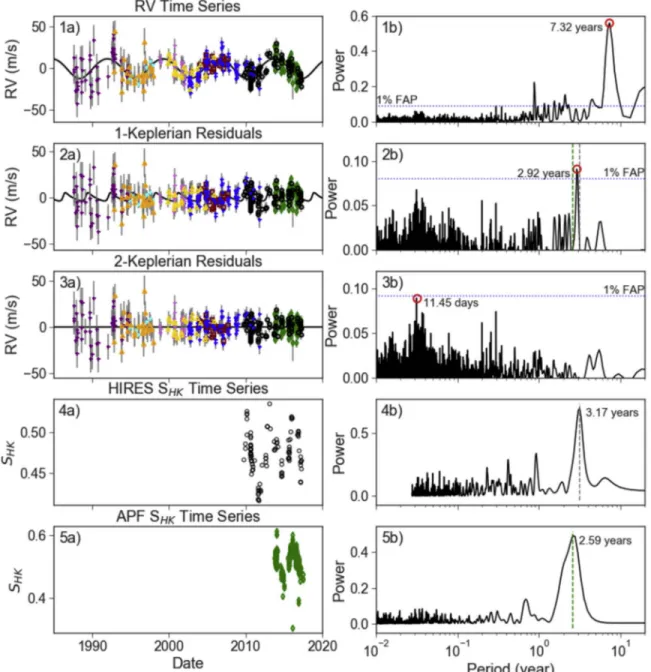
A clear periodicity of 7.32 yr dominates the periodogram of the RV data set. This is within the 1σ credible interval of the best-fit periodicity found with RadVel, which yielded a ΔBIC>200 when we tested its significance. Once the best-fit Keplerian planetary orbit from RadVel is subtracted from the RV data, the residuals and their periodogram are plotted in panels(2a) and (2b) of Figure7. The peak periodicity observed in the periodogram of the RV residuals is located at approximately 3 yr, coincident with the periodicity of the SHK

time series.

For the SHK time series, we detect clear SHK periodicities

near 3 yr, indicative of a∼3 yr magnetic activity cycle (panels (4)–(5b)). We note that the peak SHKperiodicity appears to be

slightly discrepant between the Keck and APF data sets (PKeck=3.17 yr; PAPF=2.59 yr), but consistent within the

FWHM of the periodogram peaks. This discrepancy likely results from a variety of causes, including the shorter time baseline of the APF data, which covers only a single SHKcycle,

and the typically non-sinusoidal and quasiperiodic nature of stellar activity cycles. The data sets also show a small offset in the median SHK value, likely due to differing calibrations

between the instrumental and telescope setups. However, the amplitude of the SHKvariations appears consistent between the

data sets.

We next test whether the 3 yr activity cycle could be responsible for contributing power to the 7 yr periodicity. The longer period is not an alias of the 3 yr activity cycle, nor is it in a low-order integer ratio with the magnetic activity cycle. We perform a Keplerian fit to the RV time series from HIRES and the APF, with a period constrained at the stellar activity period (1147 days). We find an RV semi-amplitude of K = 4.8 1.7m s

2.2 1

-+ - _{and a large eccentricity of 0.53} 0.27 0.24

-+ _{fits the data}

set best. We then subtract thisfit from the RV data to determine whether removal of the activity-induced RV periodicity affects

the significance of the planet periodicity. The 7 yr periodicity in the residuals is still clearly visible by eye, and a one-planetfit to the RV residuals after the activity cycle is subtracted yields a ΔBIC=197.4 when compared to a model with no planet.

We next checked the RVs for correlation with SHK. Minor

correlation was detected for the Keck/HIRES data set, with a Spearman correlation coefficient of rS=0.28 at moderate

statistical significance (p=0.01). For the APF data set, a stronger and statistically significant correlation was found (rS=0.50, p=0.01) between SHK and RV. However, given

that the 3 yr magnetic cycle shows up in the RV residuals, it is not surprising that RV and SHK might be correlated. There is

also rotationally modulated noise that might be present in both data sets near the ∼11 day rotation timescale, increasing the correlation. We attempt to determine whether the measured correlation derives from the 3 yr periodicity in both data sets, or whether it is produced by other equivalent periodicities in the RV and SHK data sets.

To test this, wefirst performed a Keplerian fit with a period of approximately 3 yr to the Keck and APF SHK time series

using RadVel. Although stellar activity is not the same as orbital motion, we used the Keplerian function as a proxy for the long-term stellar activity cycle of ò Eridani. We found a maximum probability period of 1194_-+₂₅30 days for the HIRES data and 989-+2640 days for the APF data. These periodicities are

indeed discrepant by more than 5σ. When combined, we found a period of 1147-+2022 days for the full HIRES and APF data set.

We then subtracted the maximum probability 3 yr fit from each SHKdata set, and examined the residual values. We found

that the correlation between these SHK residuals and the RV

data was significantly reduced for the APF data, with rS=0.17

and p=0.04. This suggests that the strong correlation we detected was primarily a result of the 3 yr periodicity. For the HIRES data set, the moderately significant correlation of rS=0.28 was unchanged.

A Lomb–Scargle periodogram of the SHK residuals is

displayed in Figure8. It shows no significant peak or power near the posterior planet period at 2691 days, demonstrating that the SHK time series has no significant periodicity at the

planet’s orbital period.

Our next tests involved modifying our one-planetfits to the RV data to account for the stellar activity cycle in two ways. Wefirst performed a one-planet fit to the RVs using a linear decorrelation against the SHK values for the HIRES and APF

data sets. We then performed a two-Keplerian fit to the RV data, in order to simultaneously characterize both the planetary

Figure 4.Keck/NIRC2 Ms-band vortex performance/completeness maps for a τ=5σ detection threshold for all three different ages considered here. The red curve highlights the 95% completeness contour.

orbit and the stellar activity cycle. In both cases, we checked for significant changes to the planetary orbital parameters due to accounting for the stellar activity cycle in the fit. For both tests, we find that the maximum likelihood values of the planet’s orbital parameters all agree within 1σ credible intervals with the single-planetfit.

We note that, from the two-Keplerianfit, the best-fit second Keplerian provides some information about the stellar activity cycle. It has a best-fit period of 1079 days, or 2.95 yr, shorter than the periodicity derived from afit to the HIRES and APF SHK time series. However, though the other parameters in this

fit seem to be converged, the period and time of conjunction of

the second Keplerian are clearly not converged over the iterations completed for this model. Increasing the number of iterations does not appear to improve convergence. This again points to the quasiperiodic nature of stellar activity cycles, and the different time baselines of the full RV data set and the SHK

time series available. The fit has an RV semi-amplitude of Kactivity=4.4 m s-1, lower than the semi-amplitude of the

planet at Kb=11.81±0.65 m s-1.

4.2.3. Search for Additional RV Planets

We used the automated planet search algorithm described by Howard & Fulton (2016) to determine whether additional

planet signatures are present in the combined RV data set. The residuals to the two-Keplerianfit were examined for additional periodic signatures. The search was performed using a 2D Keplerian Lomb–Scargle periodogram (2DKLS) (O’Toole et al.2009).

The residuals to the two-Keplerian fit show several small peaks, but none with empirical false alarm probabilities(eFAP) (Howard & Fulton2016) less than 1% (Figure7, panel(3b)). A broad forest of peaks at approximately 12 days corresponds to the stellar rotation period and is likely due to spot-modulated stellar jitter. The next most significant peak is located at 108.3 days. We attempted a three-Keplerianfit to the RVs with the third Keplerian initiated at 108.3 days. However, we were unable to achieve convergence in a reasonable number of iterations, and the walkers were poorly behaved. This serves as evidence against the inclusion of a third periodicity. We conclude that there is insufficient evidence to suggest an inner planet toò Eridani b exists.

RV and residual time series, as well as 2DKLS periodograms used for the additional planet search, are plotted in Figure7, panel(3a) and (3b).

4.2.4. Gaussian Processes Fits

For all of these analyses, we have assumed white noise and added a“jitter” term in quadrature to account for uncertainty due to stellar activity. We assessed whether this was reasonable by performing a one-planetfit using RadVel and including a Gaussian processes model to account for rotationally modu-lated stellar noise (S. Blunt & A. W. Howard 2018, in preparation; M. Kosiarek et al. 2018, in preparation) as well as the 3 yr stellar activity cycle.

First, we used RadVel with a new implementation of GP regression using the quasiperiodic covariance kernel tofit four

Figure 5.Performance/completeness maps for a τ=5σ detection threshold for all three different ages considered here using VLT/NACO Lp-band data (PI: Quanz, Program ID: 090.C-0777(A)) presented in Mizuki et al. (2016). The red curve highlights the 95% completeness contour.

Table 3 RadVel MCMC Posteriors

Parameter Credible Interval Maximum Likelihood Units

Pb 2691-+2829 2692 days Tconjb 2530054-+770800 2530054 JD eb 0.071-+0.0490.061 0.062 ωb 3.13-+0.790.82 3.1 radians Kb 11.48±0.66 11.49 m s−1 γHIRES 2.0±0.89 2.05 m s-1 γHARPS −4.6±1.6 −4.8 m s-1 γAPF −3±1 −3 m s-1 Lick4 g -2.45-+0.960.99 −2.41 m s-1 Lick3 g 10.5-+1.92.0 11.0 m s-1 Lick2 g 8.6±2.3 8.6 m s-1 Lick1 g 8.5±2.5 8.5 m s-1 γCES+LC 6.7±2.7 6.7 m s-1 γCES+VLC 3.2±1.8 3.3 m s-1 g˙ ≡0.0 ≡0.0 m s−1d−1 ¨ g ≡0.0 ≡0.0 m s−1d−2 σHIRES 5.99-+0.820.88 5.83 m s-1 σHARPS 5.3-+1.61.7 4.8 m s-1 σAPF 5.26-+0.720.75 5.12 m s-1 Lick4 s 7.1-+0.880.96 6.85 m s-1 Lick3 s 7.6-+1.51.7 7.2 m s-1 Lick2 s 2.8-+1.62.3 0.0 m s-1 Lick1 s 14.5-+2.12.4 13.9 m s-1 CES LC s + 9.8-+2.73.0 9.0 m s-1 σCES+VLC 4.4-+2.12.2 3.6 m s-1

Note.860,000 links saved.

GP hyperparameters in addition to the Keplerian parameters for a single planet and a white noise termσj. The hyperparameters

for the quasiperiodic kernel are the amplitude of the covariance function (h); the period of the correlated noise (θ, in this case trained on the rotation period of the star); the characteristic decay timescale of the correlation (λ, a proxy for the typical spot lifetime); and the coherence scale (w, sometimes called the structure parameter) (Grunblatt et al. 2015; López-Morales et al.2016).

We applied a Gaussian prior to the rotation period of θ=11.45±2.0 days, based on the periodicity observed in the RV residuals to the two-Keplerianfit, but sufficiently wide to allow the model flexibility. The covariance amplitudes h for each instrument were constrained with a Jeffrey’s prior truncated at 0.1 and 100m s-1_{. We imposed a uniform prior}

of 0–1 yr on the exponential decay timescale parameter λ. We chose a Gaussian prior for w of 0.5±0.05, following López-Morales et al. (2016).

The results of our GP analysis provide constraints on the hyp-erparameters, indicating that the rotation period is 11.64-+0.240.33days

and the exponential decay timescale is49 11 15

-+ _{days. The amplitude}

parameters for each instrument ranged from 0.0 to 13.4 m s-1_{, and}

were highest for the earliest Lick RV data. For some of the data sets, the cadence of the observations likely reduced their sensitivity

to correlated noise on the rotation timescale, resulting in GP amplitudes consistent with zero. For other instruments, notably the HIRES and APF data, the white noise jitter term σj was

significantly reduced in the GP model, compared with the standard RV solution.

However, when comparing the derived properties of the planet, wefind that the GP analysis has no noticeable effect on the planet’s orbital parameters. The period, RV semi-amplitude, eccentricity, time of conjunction, and argument of periastron constraints from the GP regression analysis all agree within 1σ with the values derived from the traditional one-planet fit. We therefore conclude that the rotationally modulated noise does not significantly affect the planet’s orbital parameters.

We additionally performed a one-planet fit using GP regression to model the 3 yr stellar activity cycle. For this test case, we used a periodic GP kernel because each data set covers only a relatively few cycles of the stellar activity cycle. Unlike activity signatures at the stellar rotation period, we do not expect to see significant decay or decorrelation of the 3 yr cycle over the time span of our data set. This periodic GP model had hyperparameters describing the periodicity (θ), amplitude (h), and structure parameter (w), but no exponential decay. This analysis is somewhat akin to our two-Keplerianfit, but allows moreflexibility to fit the noise than a Keplerian. For this model,

Figure 6.Time series and phase-folded radial velocity curves from all data sets are plotted. The maximum probability single-Keplerian model from RadVel is overplotted, as are the binned data(red). The plotted error bars include the internal rms derived from the RV code, as well as the fitted stellar and instrumental jitter parameterσjfor each instrument.

we placed a Gaussian prior ofθ=1147±20 days on the GP period parameter, based on the Keplerian fit to the SHK values.

We found that, when allowing each instrument its own GP amplitude parameter, h, nearly all of the instrumental amplitudes were bestfit with values very close to zero, so instead we fit for only a single GP amplitude across all instrumental data sets. We constrained this parameter with a Jeffreys prior bounded at 0.01–100 m s-1_{. We again used the w=0.5±0.05 prior for the}

structure parameter, after testing out fits at several values between 0 and 1. It remains unclear whether this was the optimal choice, given that the physical interpretation of this parameter would be different for the long-term stellar activity cycle as compared with the rotationally modulated spot noise.

The results of this analysis indicate a GP periodicity of θ=1149±17 days, a slightly tighter constraint than the imposed prior. The GP amplitude parameter was constrained to be h 4.26 1.01

1.21

= _-+

m s-1_{, comparable with the posteriors for the}

RV semi-amplitude of the second Keplerian in the two-Keplerian fit. Importantly, the model posteriors on the planetary parameters were again consistent within 1σ with our traditional one-planet fit for all parameters, including the white noise jitter terms σj as well as the orbital period, RV

semi-amplitude, eccentricity, and Keplerian angles.

We note that the traditional one-planetfit is preferred over the one-planet Gaussian processes fit by ΔBIC=19.7. The two-Keplerian fit is also preferred over the GP one-planet

Figure 7.Time series(a) and Lomb–Scargle periodograms (b). Panels (1)–(3) show the periodicities of the radial velocity measurements, residuals to a one-Keplerian (planet) RadVel fit, and residuals to a two-Keplerian (planet + stellar activity) RadVel fit, respectively. Panels (4) and (5) show the time series and periodograms of the Keck and APF SHKvalues. The peak periodicities for each data set are indicated in the periodogram plots. The periodicities of the SHKdata sets(panels 4–5) are

overplotted in the second periodogram panel(2b), showing the correspondence between SHKperiodicity and the secondary, activity-induced peak in the RV residuals.

The broad, low-significance peak at 11.45 days in panel (3b) corresponds to the stellar rotation period. Plotting symbols for the RV data sets are the same as in Figure6.

model, with ΔBIC=30.6, despite having two additional free parameters and nominally less flexibility than the GP model.

These tests demonstrate that the addition of a Keplerian or Gaussian-process model to account for stellar activity (both rotationally modulated activity and the long-period stellar activity cycle) does not strongly influence the results of the planetary orbital fit. The GP fit in particular was statistically disfavored compared to the simpler Keplerian model based on Δ BIC. We therefore choose to restrict our subsequent analyses to consider only a single planet and only white noise. Going forward, the uncertainty due to stellar activity is added in quadrature as a white-noise “jitter” term and red noise is not considered.

4.3. Combining Constraints from Imaging and RV By combining the imaging and RV data sets, it is possible to place tighter upper limits on the mass of the companion. Indeed, the RV data provides a lower limit on the planet mass (M sin i), while the direct imaging data complements it with an upper limit.

An MCMC will be used to infer the posterior on the masses and orbital parameters of the system, noted asΘ. The noise in the RV measurements dRV and in the images dDI is

independent, which means that the joint likelihood is thus separable:

dDI,dRV dRV dDI . 3

( ∣ )Q =( ∣ ) (Q  ∣ )Q ( )

4.3.1. Direct Imaging Likelihood

In this section, we detail the computation of the direct imaging likelihood(Ruffio et al.2018). The direct imaging data

dDI, temporarily shortened to d, is a vector of Nexp×Npix

elements where Nexpis the number of exposures in the data set

and Npix the number of pixels in an image. It is the

concatenation of all the vectorized speckle subtracted single exposures. A point source is defined from its position x and its brightness i. We also define n as a Gaussian random vector with zero mean and covariance matrixΣ. We assume that the

noise is uncorrelated and thatΣ is therefore diagonal

d =im+n ( )4

with m=m(x) being a normalized planet model at the position x.

Assuming Gaussian noise, the direct imaging likelihood is given by: d m d m m m d m d i x i i i i , 1 2 exp 1 2 exp 1 2 2 . 5 1 2 1 1     p S S S S = - - -µ - --

-{

}

{

}

not inferring the direct imaging covariance.

The estimated brightness i˜ , in a maximum likelihood sense,x

and associated error barσxare defined as:

d m m m ix , 6 1 1   S S = - -˜ _{( )} and m m . 7 x 2  1 1 s =₍ S- ₎- _{( )}

We can therefore rewrite the logarithm of the direct imaging likelihood as a function of these quantities(Ruffio et al.2018),

d i x i ii log , 1 2 x 2 . 8 x 2 2  s = - -( ∣ ) ( ˜ ) ( )

The definition of the planet model m is challenging when using a PCA-based image processing. Indeed, while it subtracts the speckle pattern, it also distorts the signal of the planet. The distortion is generally not accounted for in a classical data reduction such as the one used in Section4.1, which is why it is more convenient to adopt a Forward Model Matched Filter (FMMF) approach as described in Ruffio et al. (2017). The

FMMF computes the map of estimated brightness and standard deviation used in Equation (8) by deriving a linear

approx-imation of the distorted planet signal for each independent exposure, called the forward model(Pueyo2016).

We showed that the likelihood can theoretically be calculated directly from the final products of the FMMF. In practice, the noise is correlated and not perfectly Gaussian, resulting in the standard deviation being underestimated and possibly biasing the estimated brightness. We therefore recalibrate the S/N by dividing it by its standard deviation computed in concentric annuli. The estimated brightness map is corrected for algorithm throughput using simulated planet injection and recovery. The likelihood is computed for the fully calibrated S/N maps.

FMMF is part of a Python implementation of the PCA algorithm presented in Soummer et al.(2012) called PyKLIP27

(Wang et al. 2015). The principal components for each

exposure are calculated from a reference library of the 200 most correlated images from which only thefirst 20 modes are kept. Images in which the planet would be overlapping with the current exposure are not considered to be part of the reference library, to limit the self- and over-subtraction using an exclusion criterion of seven pixels (0.7λ/D). The speckle

Figure 8.Periodogram of the HIRES and APF SHKresiduals to the∼3 year fit.

The red dotted line shows the best-fit period of the planet from our initial one-planetfit. Like the SHKperiodograms shown in Figure7panels(4)–(5b), there

is no power at the planet’s orbital period. Even when the peak periodicity is removed for each data set, no additional power appears at the planet’s 7.37 year orbital period. This indicates that stellar activity is not likely to cause the 7.37 year periodicity in the radial velocity data.

27

Available under open-source license athttps://bitbucket.org/pyKLIP/ pyklip.

subtraction is independently performed on small sectors of the image.

4.3.2. Joint Likelihood and Priors

We implement a Markov-chain Monte Carlo analysis of the combined RV data from the Coudé Echelle Spectrograph, HARPS, Lick/Hamilton, Keck/HIRES, and APF/Levy instru-ments, as well as the single-epoch direct imaging data. We solve for the full Keplerian orbital parameters, including orbital inclination and longitude of the ascending node, which are not typically included in RV-only orbital analyses. Including the full Keplerian parameters allows us to calculate the projected position of the companion at the imaging epoch for each model orbit. This is necessary to calculate an additional likelihood based on the direct imaging data.

The full log-likelihood function used for this analysis is:

d d i ii v v t log , 1 2 2 2 log 2 . 9 x x i i m i i j i j DI RV ₂ 2 2 2 2 2 2 

å

The RV component of the likelihood comes from(Howard et al.2014). Here, vi=vi,inst−γinstis the offset-subtracted RV

measurement; σi refers to the internal uncertainty for each

measurement; vm(ti) is the Keplerian model velocity at the time

of each observation; andσjis the instrument-specific jitter term,

which contributes additional uncertainty due to both stellar activity and instrumental noise. In these models, each instrument’s RV offset (γinst) and jitter term (σj,inst) are

included as free parameters in the fit. A description of the direct imaging component of the likelihood is available in Section 4.3.1.

We draw from uniform distributions in log ,P logMb,cos ,i

e cos w, e sin w,Ω, mean anomaly at the epoch of the first observation, and γinst.

We place a tight Gaussian prior of M_å=0.781±0.078 M_e on the primary stellar mass, based on the interferometric results of Boyajian et al.(2012). Other groups have measured slightly

different but generally consistent stellar masses for ò Eridani. Valenti & Fischer (2005) report a spectroscopic mass of

M_å=0.708±0.067 M_e; Takeda et al. (2007) report a

discrepant spectroscopic result of M 0.856 0.08M

0.06

= -+ .

A tight Gaussian prior of π=310.94±0.16 mas is also imposed on stellar parallax based on the Hipparcos parallax measurement for this star(van Leeuwen2007). We place wide

Gaussian priors on the jitter terms, withσj=10.0±10.0 m s-1.

Large values for jitter are also disfavored by the second term of the likelihood function.

With these priors and this likelihood function, we solve for the full orbital parameters and uncertainties using the Python package emcee (Foreman-Mackey et al. 2013). For

compar-ison with the RadVel results, we perform our analysis both with and without the direct imaging likelihood. We use planet models of ages 800, 400, and 200 Myr in individual analyses, because the system’s age constraints span this range. We use the standard emcee Ensemble Sampler; each MCMC run uses 100 walkers and is iterated for more than 500,000 steps per walker. We check that each sampler satisfies a threshold of Gelman–Rubin statistic Rˆ <1.1for all parameters(Gelman & Rubin 1992; Ford2006), to test for nonconvergence. We note

that average acceptance fractions for our chains are fairly low, ≈5%–10%.

4.3.3. MCMC Results

The planet parameters derived in this analysis are consistent with those determined by RadVel. The posterior distributions for the companion mass and orbital inclination are plotted in Figure 9. The lower limit on planet mass Mbsini=0.72 0.07 MJup is constrained by the Keplerian velocity

semi-amplitude and agrees well with the RadVel results. With the RV data alone, the true mass(independent ofsini) has a poorly constrained upper limit, although high-mass, low-inclination orbits are geometrically disfavored. With the addition of the imaging nondetection constraints, the mass upper limit is improved.

Because younger planets are hotter and thus brighter, the direct imaging likelihood disfavors a broader region of parameter space when a younger age is assumed. Thus, the tightest constraints come from the youngest-aged planet models. Table4lists the planet parameters resulting from each MCMC run. We report the median and 68% credible intervals for each model.

We also calculate the posterior distribution on the position of the planet at the epoch of the NIRC2 imaging observation from the RV-only likelihood model. We check this posterior to ensure that the imaging observations were optimally timed to detect the planet at maximal separation from the star. The positional posterior distribution is plotted in Figure 11; it demonstrates that, at the epoch of the imaging observations, the separation of the planet from the star was indeed maximized. The planet would have been easily resolvable, regardless of the on-sky orientation(i.e., the longitude of the ascending node).

For these analyses, we draw companion mass uniformly in logarithmic space with bounds at 0.01 and 100 MJup. This is

comparable to placing a Jeffreys prior—a common choice of

Figure 9. Corner plot showing the posterior distributions and correlation between the companion mass and inclination for models using the RV likelihood only, as well as RV+ direct imaging likelihood with planet models of age 800, 400, and 200 Myr(a log-uniform prior).

prior for scale parameters such as mass and period(Ford2006).

This prior is also not significantly dissimilar to the mass distribution of Doppler-detected Jovian planets from Cumming et al. (2008), who found that dN M

dlogm

0.31

µ - _{, a roughly flat}

distribution inlogm.

To assess the impact of this choice, we repeat our analysis with a uniform prior on the mass, again from 0.01 to 100 MJup.

This alternative increases the significance of the tail of the mb

posterior distribution toward higher masses. Because mass and inclination are highly correlated, this effect also serves to flatten out the inclination posterior, adding more significance to lower-inclination orbits. Figure 10 shows the posteriors and correlation between the mass and inclination of the planet under the modified mass prior. The correlation plot is identical to that shown in Figure 9, and the mass posterior is not qualitatively changed. The median/68% confidence interval planet mass from the 800 Myr model is mb 0.83 0.15M

0.47 Jup

= _-+ _,

consistent within uncertainties with the mass constraint from the log-mass case at the same age. The inclination posterior has a wider uncertainty in the linear mass case(i=90°.8±48°.0) as compared to the log mass case(i=89°.2±41°.7). All other orbital and instrumental parameters have equivalent constraints in both cases. We conclude that the prior on mass does not significantly affect the results of the analysis.

5. Discussion

In this section, we discuss the impact of our joint RV-direct imaging analysis on the probable age of the system and the possible planet–disk interactions. We also discuss the prospect

of detecting additional planets with future facilities such as the James Webb Space Telescope.

5.1. Choice of Evolutionary Models

The direct imaging upper limits are model-dependent. We chose to use the COND model mostly for practical reasons. This choice was also motivated by the fact that, at the system’s age and probable planet mass, evolutionary models have mostly forgotten initial conditions such that hot and cold start models have converged(Marley et al.2007). However, COND

is arguably one of the oldest evolutionary models available. The treatment of opacities, chemistry, etc., are all somewhat outdated. For our 800 Myr case, the most probable age for the system, we also generated completeness maps using the evolutionary model presented in Spiegel & Burrows (2012),

referred to asSB12hereafter(Figure12). Because the publicly

available SB12 grid does not fully cover our age and mass range, some minor extrapolations were necessary. The result of this comparison shows some noticeable discrepancies across the range probed by our data(see Figure12). However, both

models seem to agree to within error bars at the location of the planet around 3.48 au, so the impact of the choice of evolutionary model on our joint statistical analysis is only marginal.

5.2. Constraints on the System’s Age and Inclination The planet is not detected in our deep imaging data to the 5σ threshold. According to our upper limits and RV results, the imaging nondetection indicates that the true age ofò Eridani is

Table 4 MCMC Results

RV Likelihood Only 800 Myr 400 Myr 200 Myr

Parameter Median and 68% Credible Interval

mb(MJup) 0.78-+0.120.43 0.78-+0.380.12 0.75-+0.100.19 0.71-+0.070.09 P(yr) 7.37-+0.070.07 7.37-+0.070.07 7.37-+0.070.07 7.38-+0.070.07 e 0.07 _0.050.06 -+ 0.07-+0.050.06 0.07-+0.050.06 0.06-+0.040.06 ω (°) 177-+5149 175-+5253 177-+4948 157-+5166 Ω (°) 180-+123122 184-+131126 212-+148108 276-+15847 i(°) 90 ₄₃42 -+ ₈₉ 42 42 -+ ₈₉ 3535 -+ ₉₀ 2423 -+ tperi(JD) 2447213-+429336 2447198+-361426 2447218-+407332 2447032-+402475 γLick1(m s-1) 8.4-+2.42.4 8.5-+2.42.4 8.4-+2.32.4 8.4-+2.42.4 σLick1(m s-1) 15.1-+1.82.0 15.1+-1.82.0 15.1-+1.82.1 15.1-+1.82.1 γCES+LC(m s-1) 6.9-+2.62.6 6.9+-2.62.6 6.9-+2.62.6 6.9-+2.52.6 σCES+LC(m s-1) 10.9-+2.12.5 10.9-+2.52.1 10.9-+2.22.5 10.9-+2.22.5 γLick2(m s-1) 8.5-+1.91.9 8.5-+1.91.9 8.5-+1.91.9 8.5-+1.92.0 σLick2(m s-1) 4.7-+1.32.1 4.7+-1.42.2 4.7-+1.42.1 4.8-+1.42.2 γLick3(m s-1) 10.5-+1.91.9 10.6-+1.81.9 10.5-+1.91.9 10.6-+1.81.9 σLick3(m s-1) 9.2-+1.21.4 9.2+-1.11.4 9.2-+1.11.4 9.2-+1.11.4 γCES+VLC(m s-1) 3.4-+1.81.7 3.4+-1.91.8 3.4-+1.81.8 3.4-+1.81.8 σCES+VLC(m s-1) 6.8-+1.51.8 6.8+-1.51.8 6.9-+1.51.7 6.8-+1.51.8 γLick4(m s-1) -2.4-+1.01.0 -2.4-+1.01.0 -2.4-+1.01.0 -2.4-+1.01.0 σLick4(m s-1) 8.7-+0.70.8 8.7+-0.70.7 8.7-+0.70.7 8.7-+0.70.7 γHARPS(m s-1) -4.5-+1.61.6 -4.5-+1.51.5 -4.5-+1.51.5 -4.4-+1.61.6 σHARPS(m s-1) 7.4-+1.01.3 7.4-+1.31.0 7.4-+1.01.3 7.4-+1.01.3 γHIRES(m s-1) 2.0-+0.90.9 2.0+-0.80.9 2.0-+0.90.9 1.9-+0.90.9 σHIRES(m s-1) 7.9-+0.60.7 7.8+-0.60.7 7.9-+0.60.7 7.8-+0.60.6 γAPF(m s-1) -2.7-+1.01.0 -2.7-+1.01.0 -2.7-+1.01.0 -2.7-+1.01.0 σAPF(m s-1) 7.3-+0.50.5 7.3+-0.50.5 7.3-+0.50.5 7.3-+0.50.5

likely to be closer to 800 Myr. Moreover, spectroscopic indicators of age(logRHK¢ and rotation) point toward this star

being at the older end of the age range tested here, nearer to 800 Myr than 200 Myr(Mamajek & Hillenbrand2008). VLTI

observations were used to interferometrically measure the stellar radius and place the star on isochrone tracks. These models also yield an age of 800 Myr or more(Di Folco et al.

2004). Thus, the most likely model included here is the

800 Myr model, which is also a fortiori the least restrictive in placing an upper limit on the planet mass. This model yields a mass estimate of Mb=0.78-+0.120.38MJup and an orbital plane

inclination of i=89°±42°.

We note that this inclination is marginally consistent with being co-planar with the outer disk belt, which has a measured inclination of i=34°±2° (Booth et al.2017). Although the

direct imaging nondetection naturally favors near edge-on solutions, the full posterior distribution can still be interpreted as consistent with the planet being co-planar with the outer disk. With the joint RV and imaging analysis, we are unable to definitively state whether the planet is or is not co-planar with the outer debris disk. However, we are able to rule out ages at or below 200 Myr if coplanarity is required.

To assess the properties of the planet assuming coplanarity with the disk, we repeat our joint analysis, implementing a new Gaussian prior on the inclination of i=34°±2° rather than the uninformative geometric prior used in the previous analysis.

Table 5

Keck Radial Velocity Measurements

JD RV(m s−1)a σRV(m s−1)b SHK 2455110.97985 −6.54 1.30 0.467 2455171.90825 −3.33 1.09 0.486 2455188.78841 7.90 1.11 0.481 2455231.7593 −8.39 1.13 0.497 2455255.70841 1.66 0.70 0.520 2455260.71231 1.77 1.01 0.523 2455261.71825 0.75 1.30 0.526 2455413.14376 −10.67 0.76 0.500 2455414.13849 −16.73 0.99 0.000 2455415.14082 −20.89 0.78 0.495 2455426.14477 −17.57 0.86 0.494 2455427.14813 −18.05 0.87 0.483 2455428.14758 −21.46 0.87 0.480 2455429.14896 −18.67 0.90 0.475 2455434.14805 7.21 0.86 0.474 2455435.14705 4.46 0.89 0.481 2455436.14535 −2.48 0.83 0.485 2455437.15006 −5.03 0.94 0.480 2455438.15172 −14.24 0.90 0.484 2455439.14979 −13.17 0.51 0.474 2455440.15188 −22.38 0.88 0.471 2455441.15033 −19.71 0.99 0.469 2455456.01632 4.52 0.97 0.466 2455465.07401 −12.99 0.98 0.449 2455469.1284 7.81 1.01 0.465 2455471.97444 −4.15 1.16 0.471 2455487.00413 −9.44 0.96 0.454 2455500.98687 −2.23 1.05 0.461 2455521.89317 −11.42 1.05 0.455 2455542.95125 −8.56 1.20 0.458 2455613.70363 0.65 1.01 0.466 2455791.13884 1.87 0.87 0.433 2455792.13464 −9.19 0.90 0.430 2455793.13858 −17.85 0.89 0.426 2455795.14053 −15.43 0.96 0.418 2455797.13828 −5.67 0.83 0.419 2455798.14195 −5.00 0.84 0.424 2455807.1116 −3.91 0.99 0.417 2455809.1367 −0.90 0.99 0.429 2455870.9902 1.81 1.20 0.437 2455902.82961 4.20 0.74 0.429 2455960.69933 −8.22 1.21 0.460 2456138.12976 −2.69 0.86 0.464 2456149.05961 −2.49 0.53 0.470 2456173.13157 −1.22 0.96 0.459 2456202.99824 19.64 0.71 0.507 2456327.70174 20.33 1.05 0.535 2456343.7026 16.52 1.05 0.505 2456530.11763 6.76 0.90 0.489 2456532.12218 8.06 0.85 0.479 2456587.96668 14.41 1.03 0.479 2456613.91026 15.04 1.02 0.481 2456637.81493 23.88 1.02 0.487 2456638.79118 32.35 1.07 0.491 2456674.80603 11.70 1.03 0.488 2456708.78257 2.49 0.99 0.482 2456884.13093 12.85 0.95 0.446 2456889.14678 18.51 0.82 0.466 2456890.14703 13.09 0.86 0.461 2456894.13998 8.71 0.83 0.446 2456896.11131 15.09 0.78 0.447 2456910.94964 13.84 0.64 0.450 2457234.13834 9.97 0.85 0.491 2457240.99109 6.26 0.52 0.468 2457243.14297 3.19 0.78 0.476 Table 5 (Continued) JD RV(m s−1)a _σ RV(m s−1)b S_HK 2457245.14532 5.26 0.90 0.479 2457246.14242 −1.45 0.99 0.477 2457247.14678 −5.60 1.01 0.482 2457254.14889 8.50 0.80 0.475 2457255.15244 6.36 0.91 0.466 2457256.15168 5.80 0.83 0.476 2457265.14924 5.74 0.88 0.469 2457291.04683 6.07 1.05 0.491 2457326.9831 6.10 1.12 0.501 2457353.88153 −0.55 1.09 0.519 2457378.78993 2.19 1.08 0.519 2457384.78144 14.17 1.10 0.517 2457401.75106 6.07 0.99 0.517 2457669.02614 1.91 1.10 0.497 2457672.99494 −1.33 1.20 0.497 2457678.97973 −13.88 1.10 0.495 2457704.03411 −14.12 0.67 0.501 2457712.99284 −4.84 1.18 0.478 2457789.74988 −13.12 1.12 0.439 2457790.737 −8.09 1.01 0.440 2457803.70407 −4.25 1.09 0.460 2457804.70718 −6.55 1.09 0.471 2457806.79201 −11.62 1.13 0.464 2457828.7545 −12.69 1.12 0.455 2457829.71875 −19.82 0.98 0.466 2457830.71979 −12.66 1.10 0.465 Notes. a

The RV data points listed in these tables are not offset-subtracted.

b_{Uncertainties quoted in these tables reflect the internal statistical variance of}

the spectral chunks used to extract the RV data points(see Section2.2for a full description). They do not include jitter.