Multiuser Optimal Transmit Beamforming: Performance Studies, Antennas Selection, A Genetic Algorithm Approach

(1)

MULTIUSER OPTIMAL TRANSMIT BEAMFORMING: PERFORMANCE

STUDIES, ANTENNAS SELECTION, A GENETIC ALGORITHM APPROACH

FAIKA HOQUE

DÉPARTEMENT DE GÉNIE ÉLECTRIQUE ÉCOLE POLYTECHNIQUE DE MONTRÉAL

MÉMOIRE PRÉSENTÉ EN VUE DE L’OBTENTION DU DIPLÔME DE MAÎTRISE ÈS SCIENCES APPLIQUÉES

(GÉNIE ÉLECTRIQUE) OCTOBRE 2018

(2)

ÉCOLE POLYTECHNIQUE DE MONTRÉAL

Ce mémoire intitulé :

MULTIUSER OPTIMAL TRANSMIT BEAMFORMING: PERFORMANCE

STUDIES, ANTENNAS SELECTION, A GENETIC ALGORITHM APPROACH

présenté par : HOQUE Faika

en vue de l’obtention du diplôme de : Maîtrise ès sciences appliquées a été dûment accepté par le jury d’examen constituté de :

M. FRIGON Jean-François, Ph. D., président

M. SAVARIA Yvon, Ph. D., membre et directeur de recherche

M. CARDINAL Christian, Ph. D., membre et codirecteur de recherche M. NERGUIZIAN Chahé, Ph. D., membre

(3)

DEDICATION

To my parents and sisters...

(4)

ACKNOWLEDGEMENTS

One of the joys of completion is to look over the journey past and remember all the people who have helped and supported me along this long but fulfilling road. The present work would not have been possible without the valuable help of my academic advisors.

I would like to express my sincere gratitude to my supervisor, Prof. Yvon Savaria, for his support and valuable comments during my studies at Polytechnique Montréal. His guidance and patience smoothed the path and made it possible for me to develop this thesis. It was both an honor and a privilege to work with him. His feedback on this work brought new and interesting perspectives to the problem.

I must thank my co-supervisor, Prof. Christian Cardinal for his advice and feedback during my research work. Our productive discussions helped me to elevate the quality of my research work. I am also grateful of the jury members for generously accepting to evaluate my thesis.

But most of all, I would like to thank and express my deepest gratitude to my family and friends for their continuous support.

(5)

RÉSUMÉ

La formation de faisceaux est une technique très prometteuse utilisant un grand nombre d'antennes pour transmettre un signal vers un ou plusieurs utilisateurs. L'objectif est d'augmenter la puissance du signal chez l'utilisateur souhaité et de réduire la puissance d'interférence chez les utilisateurs non visés. Étant donné que la transmission de la formation de faisceaux augmente la puissance dans une direction spécifique, cela permet à un accès multiple par division spatiale de servir plusieurs utilisateurs simultanément. Cependant, le problème est de garder un équilibre entre maximiser la puissance du signal et minimiser la puissance d'interférence dans les systèmes multi-utilisateurs. Cette thèse décrit une structure simple qui fournit une base théorique pour un système de formation de faisceau optimal. Dans cette thèse, nous étudions les propriétés des systèmes linéaires et optimaux dans différents scénarios, tels que les rapports des signaux faibles et élevés au bruit, des nombres multiple d'antennes, le canal à évanouissement de Rayleigh et les retards multiples. Nous analysons les scénarios lorsque la formation de faisceaux linéaires fonctionnent comme une formation de faisceau optimale. Ensuite, nous proposons une méthode simple pour sélectionner le nombre minimum d'antennes suffisantes pour satisfaire aux exigences de qualité de service des utilisateurs. Lorsque le nombre d’antennes à la station de base est très grand, il ne sera peut-être pas nécessaire d’utiliser toutes les antennes pour desservir seulement quelques utilisateurs. Cette situation incite à choisir un nombre d’antennes limité. Cependant, le nombre choisi peut ne pas suffire à satisfaire les exigences de qualité de service des utilisateurs en raison de fortes interférences, de conditions de canal et du nombre d'utilisateurs. Pour résoudre ce problème NP-difficile, il faut faire une recherche exhaustive ou une recherche heuristique des méthodes itératives avec un coût de complexité informatique acceptable. Ainsi, nous proposons un cadre simple pour sélectionner un ensemble d'antennes suffisantes pour satisfaire les besoins de l'utilisateur. Enfin, nous proposons un algorithme génétique pour une formation de faisceaux optimale avec une complexité d'implémentation faible. Considérant l'algorithme de réduction de branche comme une référence, nous comparons la performance de l'algorithme proposé dans différents scénarios.

(6)

ABSTRACT

Transmit beamforming is a very promising technique to transmit the signal from a large array of antennas to one or multiple users. The goal is to increase the signal power at the desired user and reduce the interference power at the non-intended users. Since transmit beamforming increases the power to a specific direction, it allows for space division multiple access to serve multiple users simultaneously. However, the problem is to keep the balance between maximizing the signal power and minimizing the interference power in multi-user systems. This thesis describes a simple structure that provides a theoretical foundation for optimal beamforming scheme. In this thesis, we study the properties of linear and optimal beamforming schemes in different scenarios such as low to high signal to noise ratio ranges, multiple number of antennas, simple Rayleigh fading channel, Rayleigh fading channel with Doppler effects. We analyze the scenarios when linear beamforming performs as an optimal beamforming. Next, we propose a simple method to select the minimum number of antennas that is enough to satisfy the quality of service requirements of the users. In case of massive number of antennas at base station, it may not be necessary to use all antennas to serve only few users. That situation motivates the selection of a set of limited number of antennas. However, the number of chosen antennas may not be enough to satisfy the quality of service requirements of the users due to strong interference, channel conditions and number of users. To solve this NP-hard problem, it requires an exhaustive search or heuristic search, iterative methods with a cost of computational complexity. Thus, we propose a simple framework to select a set of antennas that is enough to satisfy the user’s requirements. Finally, we propose a genetic algorithm for optimal beamforming with low implementation complexity. Considering the branch reduce and bound algorithm as a benchmark, we compare the performance of the proposed algorithm in different scenarios.

(7)

LIST OF FIGURES

Figure 1.1: Multi-antennas transmission ... 2

Figure 2.1: Illustration of the beamforming directions ... 7

Figure 3.1: Block diagram of the basic system model ... 14

Figure 3.2: Examples of compact regions with different shapes ... 17

Figure 3.3: Average sum rate vs. SNR, N=4, K=4... 30

Figure 3.4: Average sum rate vs. SNR, N=12, K=4... 31

Figure 3.5: Average sum rate vs. SNR, N=4, K=4 with velocity 100km/hr... 32 Figure 3.6: Average sum rate vs. SNR, N=4, K=4 with velocity 200km/hr... 33 Figure 3.7: Average sum rate vs. SNR, N=12, K=4 with velocity 100km/hr... 34 Figure 3.8: Average sum rate vs. SNR, N=12, K=4 with velocity 200km/hr... 34 Figure 4.1: Frame work to use limited antennas from massive antennas... 39

Figure 4.2: Number of antennas selected vs. number of users... 41

Figure 4.3: Average sum rate vs. number of users... 41

Figure 4.4: Average sum rate vs. number of users with best set selection and random antennas selection... 42 Figure 4.5: Flow diagram for the genetic algorithm... 46

Figure 4.6: Average sum rate vs. SNR with Genetic algorithm... 50

Figure 4.7: Average sum rate vs. SNR with Genetic algorithm with Doppler effects... 51 Figure 4.8: Example of convergence of the Genetic algorithm... 52

(10)

LIST OF ACRONYMS AND ABBREVIATIONS

SDMA Space Division Multiple Access

NP Non-Deterministic Polynomial

MRT Maximum Ration Transmission

ZFBF Zero Force Beamforming

MMSE Minimum Mean Square Error

MIMO Multiple Input Multiple Output

QoS Quality of Service

SNR Signal to Noise Ratio

SINR Signal to Interference Noise Ratio

GA Genetic Algorithm

BRB Branch Reduce and Bound

SOCP Second Order Cone Programming

MU-MIMO Multi-User Multiple Input Multiple Output SIMO Single Input Multiple Output

MISO Multiple Input Single Output

(11)

LIST OF APPENDICES

APPENDIX A - Source Code for Heuristic Beamforming... 61 APPENDIX B - Source Code for Optimal Beamforming... 64

(12)

CHAPTER 1 INTRODUCTION

1.1 Background and Objective

In wireless communications, the data is sent as electromagnetic waves through the environment (air, buildings, trees etc.) between the devices. The wireless channel distorts the signal, adds interference from other radio signals produced in the same frequency band and adds thermal background noise. As the radio frequency is the global resource for long range applications, wireless communication system should be designed to use the frequency resources as efficiently as possible. The overall efficiency and user satisfaction can be improved by dynamic allocation and management of the available resources. The spectral efficiency can be improved by allowing many devices to communicate in parallel and thus contribute to the total spectral efficiency. Modern multi antenna techniques enable resource allocation with precise spatial separation of users. It is possible to increase the received signal power to the intended user and at same time omit the interference to the other non-intended users by steering the power to a particular direction. The concept of steering the power to a particular direction is called beamforming. Transmit the signal from the multiple antennas using different relative amplitudes and phases such that components ad up constructively in desired directions and destructively in undesired directions. The beamforming resolution depends on the propagation environment and the number of transmit antennas [1]. If there is line of sight (LoS) between the transmitter and receiver, beamforming can be seen a signal beam toward the receiver as showed in Figure 1.1.

(13)

Figure 1.1: Multi-antenna transmission

Beamforming can also be applied in a non-LoS scenario if the multipath channel is known at the transmitter side. Since transmit beamforming focuses the signal energy to a specific place, it allows for multiple users to be served simultaneously. This is called space division multiple access where multiple users are spatially separated. One beamforming vector is assigned to each user and can be matched to its channel. However, the finite number of antennas may not be sufficient for all users which typically lead to leakage of signal power interfering with other users. It is very easy to design a beamforming vector that maximize the signal power to the intended user, but difficult to minimize the interference power. Thus, optimization of multiuser beamforming is a nondeterministic polynomial time (NP) hard problem [2].

In the first section, we study a simple structure of the optimal beamforming [3] with intuitive properties and interpretations. Moreover, we study the properties of linear beamforming schemes known as maximum ratio transmission (MRT), zero force beamforming (ZFBF) and minimum mean square beamforming (MMSE). We study the properties and performance of the transmit beamforming schemes in two types of channel: 1) Rayleigh fading channel assuming the channel is static for many transmitted symbols assuming the users have a fixed location 2) Rayleigh fading channel with real time scenario such as moving users that results in Doppler effects and multipaths delays. In addition, we study the properties of linear and optimal beamforming for two cases: 1) when the number of antennas is equal to the number of users and 2) when the number of antennas is much larger than the number of users.

Next, we study how many antennas we actually need to satisfy the QoS constraints in a massive multiple input multiple output (MIMO) scenario. Multiple antenna wireless communication

(14)

systems have recently attracted significant attention due to their higher capacity and better tolerance of the fading. Moreover, it allows to reduce the interference power by spatially separating the multiple users. However, increasing the number of transmit antennas enables to improve system performance at the price of higher hardware costs and computational complexity. For a system with large number of antennas arrays, this motivates developing techniques with reduced hardware and computational costs. An efficient approach to achieve this goal is to select the optimal antennas subset. In this thesis, we propose a simple antenna selection method for massive MIMO systems. The method not only selects optimum number of antennas but also guarantee to satisfy the quality of service (QoS) of each user. We perform the proposed method for two types of channel as mentioned earlier and compare the performance for both channel types.

Another important case we study is whether MRT, ZFBF and MMSE are truly optimal. The articles presented in [4], [5] show that MMSE is truly optimal only in special cases. For example, a symmetric scenario where the channels are equally strong and have well separated directivity. In fact, transmit MMSE beamforming performs well and satisfy the optimal beamforming structure in a symmetric scenario. However, ZFBF and MMSE beamforming is not optimal in asymmetric channel conditions. Another case is when users are well separated, and the number of antennas is much larger than the number of users [6]. In general, asymmetric channel conditions and low degree of diversity do not provide enough degree of freedom for MMSE and ZFBF to perform well. In such cases we truly need an optimum beamforming scheme to adjust the user performance. Hence, we propose an efficient algorithm to obtain multiuser optimum beamforming. We propose a genetic algorithm (GA) to find an optimum beamforming. Genetic algorithm is a heuristic search and optimisation technique inspired by natural evolution. We compare the performance of the proposed algorithm with branch reduce and bound (BRB) algorithm considering as the performance benchmark. We also analyze the implementation complexity of the proposed algorithm and show which parameters increase the complexity as well as the performance of the proposed algorithm.

(15)

1.2 Chapter Outline

The contributions of this work are folded in three sections:

 Performance studies of the linear beamforming and optimal beamforming in simple fading channels and fading channels with Doppler effects and path delays. Moreover, the effect of very large arrays of antennas on performance metric is reviewed.

 In case of large arrays of antennas, we investigate how the number of unnecessary antennas can be reduced to minimize computational complexity.

 We propose an efficient algorithm to find the optimal beamforming solution with low implementation complexity.

The remainder of this thesis is organized as follows. Chapter two describes the existing works. Chapter three presents the system model, problem formulation and a simple structure of the optimal beamforming. Moreover, the chapter shows the simulation results, our contributions in two different sections and discussions of the results. Chapter four proposes an efficient genetic algorithm for multi user optimum beamforming. Chapter five concludes by summarizing the work done and the main results reported in this thesis.

(16)

CHAPTER 2 LITERATURE REVIEW

Multiuser multiple input and multiple output (MIMO) has been extensively studied as one of the key spectral efficiency technologies. Multiple antennas at the base station (BS) enable simultaneous transmissions to multiple users to increase cell capacity. Due to the simplicity of the implementations and near optimal performance, linear beamforming techniques such as maximum ratio transmissions (MRT) [7], [8], zero force beamforming [9], [10], and minimum mean square beamforming (MMSE) [11], [12], are developed for MU-MIMO systems. The following parts explain when and why linear beamforming approaches based on MRT, ZFBF and MMSE are close to optimal and their limitations in different scenarios.

Consider a base station with antennas communicating with single antenna user devices. The channel to user is represented in the complex baseband by the vector . The channel vectors is known as the channel state information and is assumed to be perfectly known at the base station. The data signal to user is denoted and is normalized to unit power. The different data signals are separated spatially using the linear beamforming vectors where is associated with user . The complex-baseband received signal at _user

is given by the linear input and output model,

Where is the additive receiver noise with zero mean and variance . The beamforming concept of maximum ratio transmission was introduced in [7] to maximize the signal to noise ratio (SNR) at each user.

MRT is the counterpart of maximum ratio combining in receiving process.

(17)

MRT can be viewed as a matched filter where the gain of each entry in equals the relative strength of the corresponding channel coefficient in and the phase makes the signal contribution from each channel coefficient add up constructively. The inner product _is

therefore maximized which protects the useful signal against channel fading. MRT is the optimal beamforming direction for . However, when there are multiple users, it is not an optimal beamforming because the inter-user interference is uncounted for the MRT beamforming.

Zero forcing refers to signal processing that completely eliminates interference. This can be achieved at the transmitter side by selecting beamforming vectors that are orthogonal to the channels of non-intended users [9]. A theoretical motivation is that zero-forcing simultaneously minimizes the mean square error (MSE) between the received signal and the transmitted symbol. Considering the beamforming matrix and the channel matrix _,

ZFBF is the counterpart of zero-forcing filtering in receive processing. To cancel all inter-user interference, the beamforming directions are achieved by projecting the channel vector of the intended user onto the orthogonal complement of the non-intended users. ZFBF provides the optimal beamforming directions at high signal to noise (SNR) regime. Moreover, the loss in signal power due to interference cancelation typically diminishes as the number of transmit antennas increased.

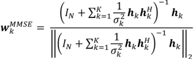
The linear MRT and ZFBF follows from straight extensions of the corresponding criteria for receiver combining such as maximize SNR and minimize the interference power respectively. Wiener filtering balances between signal power maximization and interference power minimization known as minimum mean square error beamforming (MMSE) [10],

(18)

With the total power P constraint equation (2.5) can be written,

ZFBF and MMSE beamforming are optimal when the channels are equally strong and the case when . However, when the channel conditions are varying, and number of antennas are not enough, MMSE and ZFBF can not provide an optimal solution.

(19)

The assumption of the conventional MMSE beamforming that all users have the same average SNR is clearly invalid in the case of random geometry of the cellular users. A generalized MMSE beamforming which mitigates the practical issues of the conventional MMSE is proposed in [13]. The articles [13] derived the closed form expressions of the generalized MMSE beamforming using convex optimization techniques. The system utilizes the received average SNR that contains the effects of both transmit power and path loss. The problem of joint downlink beamforming in a power-controlled network is proposed in [14], assuming that independent data streams are to be transmitted from a multiantenna base station to several decentralized single-antenna terminals. The total transmit power is limited and channel information (possibly statistical) is available at the transmitter. The design goal is to jointly adjust the beamformers and transmission powers according to individual SINR requirements. In this context, there are two closely related optimization problems. P1: maximize the jointly achievable SINR margin under a total power constraint. P2: minimize the total transmission power while satisfying a set of SINR constraints. In [14], both problems are solved within a unified analytical framework. Problem P1 is solved by minimizing the maximal eigenvalue of an extended crosstalk matrix. The solution provides a necessary and sufficient condition for the feasibility of the SINR requirements. Problem P2 is a variation of problem P1. An iterative strategy is proposed for minimizing the maximal eigenvalue of the extended coupling matrix was derived. The iteration sequence was shown to be monotone and globally convergent.

A general framework for modeling single cell, multi-cell scenarios coordinated beamforming, interference channels, cognitive radio and spectrum sharing is proposed [15]. The performance of multicell systems depends on the resource allocation such as power, frequency and spatial resources are divided among users. The tutorial [15] provides a pragmatic foundation for resource allocation where the system utility metric can be selected to achieve feasibility. Resource allocation is formulated as multi-objective optimization problem and the boundary of the performance region is also represented as efficient solutions. The multi-objective resource allocations problem is solved with poly block outer approximation algorithm. Although the algorithm converges, the worst-case convergence speed is generally exponential in the number of users . The number of antennas N and power constraints P will however have much smaller impact on the convergence scaling of the PA algorithm, as it approximates the K dimensional performance region. The main computational complexity lies in the bounding procedure which

(20)

includes a quasi-convex line-search. In practice, it might be necessary to stop the algorithm before it converges. Later, the tutorial also proposed branch reduce and bound algorithm to obtain the optimal solution. This formulation of the algorithm is a slight modification of the algorithm in [16], where the generic BRB algorithm from [17] is adapted for multi-cell resource allocation. Other adaptations are available in [18, 19, 20], where another bounding procedure is used. The system model of [18] is less general than [16], while [19, 20] are limited to single-antenna transmitters but can handle multi-cast transmissions. The convergence of the BRB algorithm to the global optimum was established in [17] and the following theorem originates from [16]. Both algorithms have a worst-case complexity that increases exponentially with the number of users K thus, both algorithms are unsuitable for real-time applications and only practically useful for solving problems with a small number of users.

A more precise and simple structure of optimal beamforming is presented in [3]. The structure provides a theoretical foundation for practical low-complexity beamforming schemes. The lecture shows the properties of linear beamforming schemes such as MRT, ZFBF, transmit MMSE and optimal beamforming based on BRB algorithm. We study the properties of different beamforming schemes based on the beamforming structure presented in [3]. An important observation from that article is when there are many more antennas than users , it makes the need for optimal beamforming. With a very large arrays where the number of antennas goes high, the linear beamforming schemes that is MMSE and ZFBF schemes performs as same as optimal beamforming in the low to high SNR range.

However, the main limitation of increasing the number of transmit and receive antennas is typically not the number of sensors but the cost of the corresponding RF channels for these antennas and the high complexity required for signal encoding and decoding. This limitation may be more severe when there are some power constraints. A promising way of capturing a large portion of the channel capacity in MIMO systems at reduced hardware costs and computational complexity is to select optimally a small number of “best” antennas from the larger set of antennas available. Antennas selection algorithms [21] [22] [23] are based on channel quality, minimum transmission power consumption, maximum throughput as performance metric has been performed in the previous literatures.

(21)

Let consider the number of selected antennas is . To select the best set of antennas, the channel quality or the performance metrics such as maximum sum throughput, minimum transmission power has to be computed for possible combinations of them. Antenna subset selection has been studied in the literature [24], [30]. Some of these studies focused on system model such as multiple input single output (MISO), single input multiple output (SIMO), multiple input and multiple output (MIMO). In case of SIMO [25] [26], selection has been made based on the signal power considerations for the receive antennas. Norm based selection method has been used MISO environment in [27], [28]. Indeed, the NBS algorithm has a very low complexity of , but it is clarified in [29] that the main drawback of this algorithm is that it may lead to a much lower capacity than that achieved by the optimal selection procedure in scenarios when some rows of the channel matrix are close to be linearly dependent. A promising approach for the fast antenna subset selection was proposed in [29]. This algorithm finds a near-optimal selection of receive antennas based on the capacity maximization. The algorithm begins with the full set of antennas available and then removes one antenna per step. In each step, the antenna with the lowest contribution to the system capacity is removed. The reduction in capacity due to removing of each single antenna is evaluated using a proper updating formula. This process is repeated until the required number of antennas remains. The complexity of this approach is . A novel fast near optimal antenna selection algorithm was proposed in [30]. The algorithm starts with empty set of selected antennas and then adds one antenna per step to this set. In each step, the antenna with the highest contribution to the system capacity is adds to the set of selected antennas. Only the receive antennas selection case will be considered until the full set of transmit antennas is used ( ).

The problem of joint multicast beamforming and antenna selection has been addressed in [22]. It is shown that the mixed norm squared is a prudent group-sparsity inducing convex regularization, in that it naturally yields a suitable semidefinite relaxation to solve the NP hard problem. The paper also indicated that the proposed algorithm significantly reduces the number of antennas required to meet the prescribed quality of service level. The algorithm iteratively run the weighted norm algorithm to find a solution for the given number of limited antennas .

Then the algorithm solve a semidefinite relaxation programming problem of transmit power minimization problem and use binary search algorithm to find a solution of parameter in

(22)

relaxation problem that gives the required number of antennas . Then the algorithm use randomization technique to generate candidate sets of beamforming vectors and choose the set that yields a minimum power solution among all candidate sets.

Joint network power minimization and base station selection scheme for cloud RAN is proposed in [31]. The paper proposed a greedy selection algorithm which selects one base station to switch off at each step. To select the base station to be switched off that maximizes the reduction in the network power consumption at each step. However, the greedy selection algorithm induces complexity exponentially with the number of base stations. To further reduce the complexity, the paper proposed three stages group sparse beamforming (GSBF) framework, by adopting the weighted mixed norm to induce the group sparsity for the beamformers. By applying the

mixed norm to induce group sparsity, the additional prior information that is transport link

power consumption, power amplifier efficiency, and instantaneous effective channel gains to design the weights for different beamformer coefficient groups, resulting in a significant performance gain. Two GSBF algorithms with different complexities are proposed: a) a bi-section GSBF algorithm and b) an iterative GSBF algorithm. Using the weighted mixed norm as a replacement for the objective function, the algorithm minimized the weighted mixed

norm to induce the group sparsity for the beamformer. Then the base stations are switch off under given priorities. The priorities are given with smaller coefficients that is measured by norm. Moreover, other system parameters that indicate the priority to be switched off is the channel power gain. Therefore, the channel power gain contributes more to the sum capacity and it provides a higher power gain and should not be encouraged to be switched off. Different from the aggressive strategy in the bi-section GSBF algorithm, which assumes that the RRH should be switched off as many as possible and thus results a minimum transport network power consumption, we adopt a conservative strategy to determine the final active RRH set by realizing that the minimum network power consumption may not be attained when the transport network power consumption is minimized.

The performance of antenna selection-based MIMO networks with large but finite number of antennas and receivers are proposed in [23]. The paper proposed genetic algorithm to select the

(23)

antennas with sum throughput as objective function and zero forcing precoder at base station. The paper showed that genetic algorithm can be implemented with different objective function and precoding method.

Genetic algorithm has been proposed [38] for MIMO systems to obtain the position and orientation of each MIMO array antenna that maximizes the ergodic capacity for a given propagation scenario. One challenging task in the MIMO system design is to accommodate the multiple antennas in the mobile device without compromising the system capacity, due to spatial and electrical constraints. Based on an interface between the antenna model and the propagation channel model, the ergodic capacity is considered as the objective function of the MIMO array optimization. The goal is to find an optimal or a suboptimal configuration for antenna position and orientation that maximizes the ergodic channel capacity. Assuming an array of dipoles and a channel model that interfaces the propagation environment with the antenna array response pattern, the GA manages to find, for each antenna, the best position and orientation subject to a space constraint. Due to the nature of GAs, the proposed method is very general. It can incorporate different types of antenna models, and it can be also used in different propagation channel models.

In [32], the authors resort to GA-based optimization to find channel parameters such as multipath attenuations and delays. In [33], a GA is used for blind channel estimation. The study reports that the GA method can offer better channel estimation accuracy than traditional methods. A similar approach was also proposed in [34]. Recently, a GA has been used to find good antenna element positions in sparse MIMO radar arrays [35] by minimizing the sidelobes of the radar pattern. Another recent work [36] used a GA to find the optimal distribution of a 3 × 3 MIMO system for an indoor propagation channel. An interesting aspect of that work is the inclusion of electromagnetic coupling in the model. However, the work does not show either which distributions were found or how the distributions change according to different multipath channel parameters. The work in [37] defends the idea of using nature-inspired methods for MIMO antenna design, but the works mentioned in the proposed work deal with the problem of antenna geometry definition and not antenna array topology for different propagation environments. Opportunistic beamforming is exploited in independent time-varying channels across multiple users [39]. The diversity benefit is exploited by tracking the channel fluctuations of the users and

(24)

scheduling transmissions to users when their instantaneous channel quality is near the peak. The diversity gain increases with the dynamic range of the fluctuations and is thus limited in environments with little scattering and/or slow fading. The paper proposed a scheme that induces random fading when the environment has little scattering and/or the fading is slow. Moreover, the article focused on the downlink of a cellular system. The paper used multiple antennas at the base station to transmit the same signal from each antenna modulated by a gain whose phase and magnitude is changing in time in a controlled but pseudorandom fashion. The gains in the different antennas are varied independently. Channel variation is induced through the constructive and destructive addition of signal paths from the multiple transmit antennas to the (single) receive antenna of each user. The overall (time varying) channel signal-to-interference-plus-noise ratio (SINR) is tracked by each user and is fed back to the base station to form a basis for scheduling. The proposed scheme can be viewed as opportunistic beamforming as the transmit powers and phases are randomized and transmission is scheduled to the user which is close to being in the beamforming configuration. The main idea is to amplify the multiuser diversity gain by inducing faster and larger fluctuations.

(25)

CHAPTER 3 SYSTEM MODEL AND PROBLEM ANALYSIS

3.1 System Model

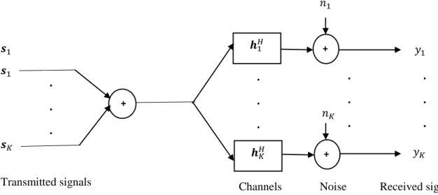
Consider a single cell scenario where a base station equipped with antennas communicates with user devices, as shown in Figure 3.1. The users are assumed to have single effective antenna. This scenario can be viewed as the superposition of several multiple input single output links (MISO). Thus, it is also known as multi-users MISO communication. The channel to

user is assumed to be flat fading and represented in the complex baseband by the vector

_{. The channel vectors [} _{] are non-correlated to each other. The complex}

valued element describes the channel from the transmit antenna to user. Its magnitude represents the gain (or attenuation) of the channel. We assume that the channel vector is quasi-static that is constant for the duration of many transmission symbols. The channel vectors is known as the channel state information and is assumed to be perfectly known at the base station. The data signal to user is denoted and is normalized to unit power. The different data signals are separated spatially using the linear beamforming vectors where is associated with user . The normalized version is called the

beamforming direction. The squared norm is the power allocated to the _user.

Figure 3.1: Block diagram of the basic system model for a downlink single cell

+ + Noise Channels + . . . . . . . . .

Transmitted signals _Channels _{Received signals} . . .

(26)

Under these assumptions, the complex-baseband received signal at user is given by the linear input and output model,

Where is additive receiver noise with zero mean and variance .

3.2 Resource Allocation Problem

The performance of multi-cell systems depends on the resource allocation such as, how the time, power, frequency, and spatial resources are divided among users. The concept of resource allocation is defined as allocating transmits power among users and spatial directions, while satisfying a set of power constraints that have physical and economic implications. A major complication in resource allocation is the inter-user interference that arises and limits the performance when multiple users are served in parallel. This section formulates the general optimization problem, discusses the solution strategy in later sections, and derives some basic properties of the optimal solution and the performance region.

3.2.1 The Power Constraints

The power resources available for transmission need to be limited somehow to model the inherent restrictions of practical systems. With the total power budget and the average transmit power allocated to the _{user, the power constraint can be defined as,}

Where serves as an upper bound on the allowed transmit power in the subspace spanned by . The allocated transmit power might be the same for all users, but can also be used to define subspaces where the transmit power should be kept below a certain threshold when transmitting to a specific user.

(27)

3.2.2 User Performance

To enable low complexity, we assume single user detection that means a user is not attempting to decode and subtract interfering signals while decoding its own signals. This assumption places the responsibility for interference control at the transmitter-side, where the computational resources are available. The corresponding SINR for user

The performance is measured by an arbitrary continuous function of of the SINR. With this definition, it is preferable for to have a large positive value on because it corresponds to good performance. Ideally, the function should be selected to quantify the performance quality in a way comprehensible to the user and the system provider. Here, we follow a common example of user performance that is information rate. The achievable information rate is and describes the number of bits that can be conveyed to user k (per channel use).

3.2.3 Multi-Objective Resource Allocation

Each user has its own objective to be optimized, thus there are different objectives that typically are conflicting. Without loss of generality, our resource allocation problem is formulated as,

(28)

The optimization problem can be interpreted as searching for a transmit strategy that satisfies the power constraints and maximizes the performance of all users. Since the performance of different users is coupled by both power constraints and inter-user interference, there is generally not a single transmit strategy that simultaneously maximizes the performance of all users. For example, in (3.3) improves if less interference is caused to

_{user but decreasing the interference at}_{that typically requires decreasing the useful signal}

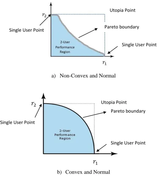
power at other users and thereby degrading their SINRs. To study the conflicting objectives of a multi-objective optimization problem, it is instructive to consider the set of all feasible operating points in (3.4) [38], which we call the performance region.

a) Non-Convex and Normal

b) Convex and Normal

Figure 3.2: Examples of compact regions with different shapes Single User Point

Single User Point Utopia Point

Single User Point

Single User Point Utopia Point

Pareto boundary Pareto boundary

(29)

This region describes the performance that can be guaranteed to be simultaneously achievable by the users. The dimensional performance region is denoted as ℛ and its shape depends strongly on the channel vectors and power constraints as shown in Figure 3.2

The utopia point u is the unique solution to (3.4) in degenerate scenarios when the optimization decouples and all users can achieve maximal performance simultaneously. In general, ℛ and represents an unattainable upper bound on performance. There are some tentative solutions in ℛ that are not dominated by any other feasible point. These points are called Pareto optimal and are such that the performance cannot be improved for any user without decreasing for at least one other user.

We outline the proof from [3] and [15]. For any given ℛ with also belongs to ℛ. To this end, let be a feasible transmit strategy that attains and consider the alternative transmit strategy , where is a set of power allocation coefficients that should belong to

Obviously, the point r is achieved by selecting . To prove that a given is also belongs to ℛ we need to find that gives this point. This corresponds to the conditions which can be formulated as linear equations and solved using the approach in [50]. Finally, the existence of for any can be proved using interference functions [51].

3.3 Subjective Solutions to Resource Allocation Problem

Recall that the Pareto boundary of the performance region contains all tentative solutions in (3.4), where each representing a certain tradeoff between the users performance. Whenever the utopia points outside of the performance region, there is no objectively optimal resource allocation. To actually compare the merits of different Pareto optimal points, the system designer (or decision maker) needs to bring its own subjective perspective on system utility.

Based on a system utility function, the multi-objective optimization problem in (3.4) can be converted to the following single objective optimization problem (P1),

(30)

Problem P1 is very hard to solve. The article in [48] proves that equation (3.6) is a NP hard problem for many common utility functions. For example, the sum rate, . This problem has a single (non-unique) solution, because the system utility function resolves the conflicting interests in the multi-object problem. The selection of is therefore very important and should be based on a profound knowledge of performance region ℛ. Moreover, all utility functions are subjective by nature, because each function imposes a certain order of vectors in the performance region. This formulation shows that resource allocation means searching that optimizes system utility.

3.3.1 Convex Optimization for Resource Allocation

In this section we study under which conditions the single objective resource allocation problem in (3.6) is linear, convex. These problems can be solved efficiently using interior point methods. [49], [50]. The problem (3.6) has convex constraints. Therefore, the classification strongly depends on the cost function which unfortunately is a complicated function that seems a non-convex. The cost function depends on the SINRs which are non-convex functions of the beamforming vectors [ ]. To pinpoint the main cause of non-convexity, [15] represent the SINRs by auxiliary optimization variables such that , equation (3.6) rewrite as,

(31)

The second row of (3.7) represents the auxiliary SINR constraints the optimal solution always gives equality in these constraints. The main complication lies in the SINR constraints, because is a convex function with respect to ( . In other words, it is generally the SINR constraints that prevent (3.7) from being a convex problem. These constraints are non-convex because of the multiplication between (the SINR value at _{user) and (the inter-user interference caused to} _{user). Three approaches to}

resolve the non-convexity can be envisioned.

(1) Fix the inter-user interference caused to each user (2) Fix the SINR value at each user

(3) Turn the multiplication into addition by change of variables

None of these approaches can be applied successfully to any resource allocation problem, but they will help identifying special cases when (3.6) has a hidden convex structure and thus can be solved efficiently. The existing work [15], [3] consider the second approach for achieving convex formulations.

3.3.2 Minimize the Transmission Power with Fixed Quality of Service Requirements:

As a preparation toward to solve the (3.6), we first solve the relatively simple power minimization problem as outlined in [3], [15]. Power minimization problem (P2) is formulated as follows,

Consider the case when the system designer knows exactly which performance each user should be allocated that is the optimal SINR values . Now if we set , and solve P2 for these particular parameters, the beamforming vectors that solve P2 will now also solve P1. As described in [3], [15] (3.8) finds beamforming vectors that achieves the SINR

(32)

values . The solution to P1 must satisfy the total power constraint in (3.6), because (3.8) gives the beamforming that achieves the given SINRs using the minimum amount of power. Since the beamforming vectors from P2 are feasible for P1 and achieve the optimal SINR values, they are optimal solution to P1 as well. The difference between the relatively easy P2 and the difficult P1 is that the SINRs are predefined in P2 while we need to find the optimal SINR values along with the beamforming vectors in P1

3.3.3 Solution to Transmission Power Minimization with SINR Constraints

Problem P2 can be reformulated as a convex problem [31]. The cost function is clearly a convex function of the beamforming vectors. Note the absolute values in SINR constraints in (3.8) make and _{completely equivalent for any common phase rotation}

as in [46]. Without loss of optimality, [ref] exploit this phase ambiguity to rotate the phase such that the inner product is real valued and positive. This shows that . By letting denoting the real part, the constraint can be rewritten as

The reformulated SINR constraint in equation (3.9) is a second order cone constraint, which is a convex type of constraint [46] [47].

Optimization theory provides many important properties for the reformulated convex problem. In particularly strong duality and that the Karush-Kuhn-Tucker (KKT) conditions are necessary and sufficient for the optimal solution. The strong duality and KKT conditions for P2 play a key role in this solution. To show this, define the Lagrange function of P2 as [46]

(33)

Where is the Lagrange multiplier corresponds to the SINR constraint. The dual function is and the strong duality implies that it equals the total power

at the optimal solution. KKT conditions which say that for

at the optimal solution.

Where denotes the identity matrix. The expression (3.13) is achieved from (3.12) by adding the term to both sides. Since is a scalar, equation (3.13) shows that optimal solution must be parallel to

. In other words, the optimal beamforming vectors are

Beamforming power = Beamforming direction

Where denotes the beamforming power and denotes the unit norm beamforming direction for user k. The K unknown beamforming power are computed by solving the SINR constraints in P2. This implies for k = 1,….., K. Since the beamforming directions are known, we have K linear equations and obtain the K powers as

(34)

Where denotes the element of the matrix _{. From equation (3.5) and}

(3.10), we obtain the structure of optimal beamforming as a function of Lagrange multipliers . Lagrange multiplier can be computed by convex optimization [46] or from the fixed point equations

for all [46 ], [ 47].

3.4 Properties of Beamforming Structure

For some positive parameters , the strong duality property of P2 implies , since is the optimal cost function in P2 and =1 is the dual function. Since the matrix inverse in (3.15) is same for all users, the matrix _{with the optimal}

beamforming vectors can be written in a compact form. To this end, we note that

where contains the channels and

is a diagonal matrix with the parameters. By gathering the power allocation in matrix P, we obtain

the compact equation

Where

_and

denotes the matrix square root.

In the low signal to noise ratio case, represented by , the system is noise-limited and the beamforming matrix in (3.16) converges at

(35)

Where the matrix inverse vanishes and denotes the asymptotic power allocation. This implies is scaled version of channel vector which is similar to MRT.

On the other hand, at high signal to noise ratio case, represented by , the system is interference limited. To avoid the singularity in the inverse when is small, we use the identity _{and rewrite as}

where the term vanishes when and denotes the asymptotic power allocation and _{. The solution}

in (3.15) known as channel inversion or zero forcing beamforming because it contains the pseudo inverse of the channel matrix Hence, is a diagonal matrix. Since the off-diagonal elements are of the form , the beamforming causes zero interference by projecting onto the subspace that is orthogonal to the co-user channels.

3.5 Branch Reduce and Bound Approach to Optimization of Resource

Allocation

The resource allocation problems have important property that the optimum lies on the Pareto boundary of ℛ. This property should certainly be utilized when devising a numerical algorithm for solving the problem. The naive approach would be to generate a large set of Pareto optimal points, preferably by some approach that finds Pareto optimal points with polynomial computational complexity. However, there are more intelligent and systematic algorithms than this naive approach. These algorithms concentrate on searching parts of the Pareto boundary that give large values on .

This section describes a general algorithm for solving resource allocation the branch-reduce-and-bound (BRB) algorithm from [15]. Algorithm is designed to iteratively improve a lower branch-reduce-and-bound

and an upper bound on the optimal value of (3.6). Convergence to the global optimum

(36)

is achieved in finitely many iterations, for any accuracy In general, the number of iterations scales exponentially with the number of users which is an inescapable consequence of solving a problem that generally is NP hard (3.8).

3.5.1 Lower and Upper Bounds in a Box

An essential step in the BRB algorithms is that of bounding the highest feasible performance in a box This means finding a lower bound and a upper bound on the optimal solution. These bounds represent the performance in the lower and upper corners of the box, but only if the box has a nonempty overlap with the performance region, this is equivalent to ℛ which is easily checked by solving the feasibility problem (3.8) with a as the QoS requirements.

3.5.2 BRB Algorithm

The BRB algorithm maintains a set with non overlapping boxes that surely covers the parts of the performance region ℛ where the optimal solutions lie. Iteratively, the algorithm is split into certain boxes and bounds the performance in these new boxes for the purpose of improving a lower bound and an upper bound on the optimal value of (3.6). To aid this process, a local feasible point and a local upper bound are stored for each box .

Initially, or a box where could be the utopia point or some other optimistic point that guarantees ℛ . The initial upper bound is , while the lower bound is initialized as for some known feasible point.

Each iteration of the BRB algorithm consists of three steps: 1) Branch : Divide a box into two new boxes

2) Reduce : Remove parts of these new boxes that cannot contain optimal solutions

3) Bound : Apply the bounding procedure to one of the new boxes to improve local and global solutions.

Branch: First, is divided into two disjoint boxes and . is bisected along its

(37)

where , , and is the column of the identify matrix The local feasible points and upper bounds of , can be selected as,

and the local upper bounds can be selected as

Reduce : Next, the new boxes for are reduced by removing parts that cannot contain the optimal solution that is, parts that either give performance below the lower bound or above the local upper bound If then will not contain

the optimal solution and can be removed. Otherwise, all points satisfying are also contained in where

Bound: Each iteration ends by a search for better bounds. First, it is checked if there are any feasible points in , or if ℛ

(38)

The intersection ℛ if Otherwise, the existence of feasible points in can be checked by solving the feasibility problem (3.8) with as the QoS requirements. If ℛ , the BRB algorithm applies the bounding procedure as following

as the search curve and using line search accuracy . The normalization ensures that the line search accuracy is a global measure, thus the bounding procedure becomes faster as the boxes get smaller.

Finally, the global lower bound is updated as and the global upper bound is updated as . The stopping criterion is checked at the end of each iteration.

3.6 Heuristic Beamforming

A classic scenario in signal processing is the detection of a scalar data symbol which is observed under channel distortion, additive interference and white noise. If multiple channel observations are available for a certain data symbol, the scenario can be written as,

where is the channel symbol The symbol can be estimated from the vector valued observation as using a linear received combining filter .

Three classic receive combining techniques are:

(1) Maximum ratio combining: Weighs and aligns the observations as

to

maximize the ratio between received signal power and noise power.

(2) Zero forcing filtering: Removes interference by projecting the observations as , which is the orthogonal complement of the interfering signals. This maximizes the ratio between received signal power and interference power.

(39)

(3) MMSE filtering: The mean square error (MSE) minimizing

2 ) 1 that balances between maximizing signal power and suppressing interference.

3.6.1 Power Allocation

The previous subsection defined MRT, ZFBF and MMSE as heuristic ways of selecting the beamforming directions . When these have been selected, the power allocation ultimately determine the operating point in the performance region that is achieved by the heuristic transmit strategy. For given the SINR become

with fixed for all . The power allocations can be formulated by so called waterfilling solutions

where λ is the Lagrange multiplier.

3.7 Performance Studies in Fading Channel

In this section, we have studied the performance of MRT, ZFBF, MMSE and optimal beamforming based on BRB algorithm in two types channel: 1) Rayleigh fading channel assuming that channel is static as receivers are not moving 2) Rayleigh fading channel with proper effects due to moving receivers.

3.7.1 Simulation Environment

To solve the second order cone program (SOCP), CVX is used. CVX is a MATLAB-based modeling system for convex optimization problem [44].

a) What is CVX: CVX is a Matlab-based modeling system for convex optimization. CVX turns Matlab into a modeling language, allowing constraints and objectives to be specified using standard Matlab expression syntax. Structure of convex problem,

(40)

In CVX, cvx_begin variables x(n) minimize (f0(x)) subject to f(x)<=0 cvx_end where and must be convex.

Return values: Upon exit, CVX sets the variables  x – solution variables (s)

 cvx_optval – the optimal value

 cvx_status – solver status (Solved, Unbounded, Infeasible)

CVX uses SeDuMi, a MATLAB implementation of second order interior point methods for the actual computations [45]. The algorithms are tested with two channel types: Rayleigh fading channel, and a Rayleigh fading channel with Doppler effects. Throughout this section, the noise variance for all users is set to The results are obtained for 100 different Rayleigh channel realizations, and the SNR is measured as .

BRB algorithm is built upon solving a series of convex feasibility problems with QoS requirements. To achieve certain accuracy = 0.01 on the optimal solution, the average number of such feasibility evaluations is 3000 and the number of iterations is 2000 [15]

(41)

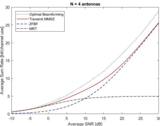
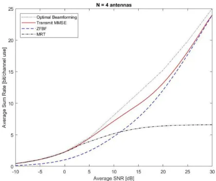
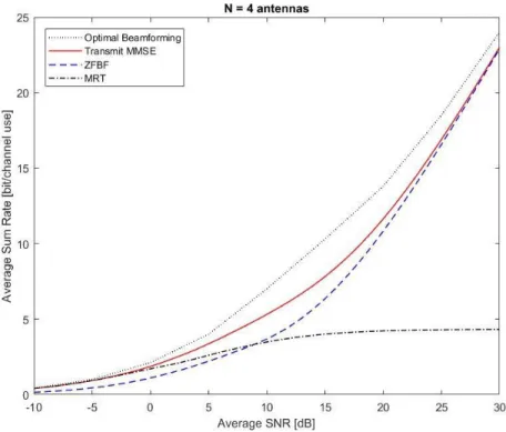
3.7.2 Rayleigh Fading Channel: Sum rate performance measurement a) In case users K=4, N=4:

The properties of MRT, ZFBF, MMSE and optimal beamforming are illustrated by simulation in Figure 3.3 We consider K=4 users for this scenario and evaluate the sum rate as utility function: . Figure 3.3 shows the simulation results for the case N=4 where MRT performs near-optimal at low SNRs, while ZFBF is optimal at high SNRs. MMSE beamforming combines the respective asymptotic properties of MRT and ZFBF with good performance at entire SNRs range. However, there is still significant gap to the optimal solution which is computed by the branch reduce and bound (BRB) algorithm whose computational complexity grows exponentially with K. The significant performance of optimal beamforming is obtained by adjusting the K=4 parameters .

(42)

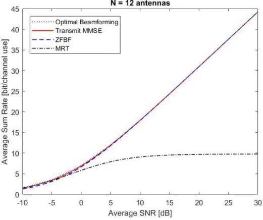
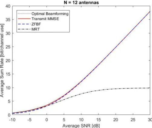
b) In case users K=4, N=12:

Massive MIMO has been received much attention to increase the sum throughput. A key motivation is that squared channel norms are proportional to , while the cross products increase more slowly with . Hence the user channel becomes orthogonal as which reduces interference and allows for less transmit power. Note that _{for large since only the elements} _{grow with .}

Figure 3.4 shows the case when number of antennas are larger than the users, . Since there are many more antennas than the users, the need for the optimality becomes much smaller.

Figure 3.4: Average sum rate vs. SNR for N=12, K=4

An important observation is transmitting MMSE beamforming and ZFBF is almost same as optimal beamforming for a system with very large antennas.

(43)

3.7.3. Rayleigh Fading Channel with Doppler effect: Sum rate performance measurement a) In case users K=4, N=4:

Figure 3.5 - 3.6 show the average throughput versus SNR for the case with different Doppler effects. Figure 3.5 shows the performance for receiver’s moving 100km/hr using a carrier frequency of 2GHz. The symbol duration is considered as

since in LTE each subframe lasts 1ms and contains 14 OFDM symbols and the sampling rate is _{with an oversampling factor . Figure 3.6 shows the performance for}

the speed 200k/hr. Simulation results show the fact that Doppler effect degrades performance compare to channel with no effect. For the speed 100km/hr and 200km/hr, the performance degrades almost 11% and 15% compare to the performance with no speed.

(44)

Figure 3.6: Average sum throughput vs. SNR with velocity, km/hr

b) In case users K=4, N=12

Figure 3.7 – 3.8 show the average throughput versus SNR for the case with different Doppler effects. Simulation results in Figure 3.7 and Figure 3.8 correspond to cases where we increase the speed to the 100km/hr and 200km/hr. They show the variation of the performance degradation that is almost the same and which is 13% when compared to the performance when the mobile is not moving.

(45)

Figure 3.7: Average sum throughput vs. SNR with velocity, km/hr

(46)

To conclude this chapter, when the number of antennas is equal to the number of users, that is when , the Doppler effect or multipath delays effect significantly reduce the performance compared to the case . Moreover, a large number of antennas reduces the necessity of optimal beamforming but it produces a huge implementation complexity with the number of users .

(47)

CHAPTER 4 PROPOSED ALGORITHMS FOR TRANSMIT

ANTENNAS SELECTION AND OPTIMAL BEAMFORMING

4.1 An Iterative Solution for Transmit Antennas Selection and Optimal

Beamforming

The more antennas at the transmitter or the receiver are equipped with, the better the data rate/link reliability. However, massive MIMO implies challenges such as hardware impairments and signal processing complexity which may limit the number of antennas in practice. Thus, it is interesting to analyze MIMO networks in the presence of large but finite number of antennas. Particularly, several antenna selection algorithms are presented in which only a set of antennas are activated based on the channel quality, transmit power to utilize the diversity of large MIMO systems. In the following section we will consider antenna selection scheme and investigate the performance of MMSE, ZFBF and MRT beamforming schemes.

Many works have done on antennas selection strategies for massive MIMO. For example, joint antenna selection and power minimization problem in [22], [31], antennas selection for a continuous and burst communication [23]. Literature studies shows that the antenna selection is a NP hard problem. To solve the NP hard problem, [31] proposed heuristic searching algorithms where the complexity increase with the number of total antennas, . Similarly, [22], [31] proposed , norm to obtain a sparse solution of the antennas selection problem. However,

all of these proposed schemes have computational complexity to select the best set of antennas as the total subsets which is increased with the value .

We propose a simple framework to select the number of antennas among the total number of antennas instead of searching a best set of antennas among all subsets as proposed in earlier work.

4.1.1 Basic Model and Problem Formulation

Assuming the same system model defined in chapter three that is a single base station with multiple antennas and single antenna receiver. The different data signals are separated spatially using the linear beamforming vectors and the transmission power is allocated to the user . The received signal at user is given by,