O
pen
A
rchive
T
OULOUSE
A
rchive
O
uverte (
OATAO
)
OATAO is an open access repository that collects the work of Toulouse researchers and
makes it freely available over the web where possible.
This is an author-deposited version published in :
http://oatao.univ-toulouse.fr/
Eprints ID : 12555
To link to this article : DOI :10.1016/j.cag.2013.05.024
URL :
http://dx.doi.org/10.1016/j.cag.2013.05.024
To cite this version : Canezin, Florian and Guennebaud, Gaël and
Barthe, Loïc
Adequate Inner Bound for Geometric Modeling with
Compact Field Functions
.(2013) Computer & Graphics, vol. 37 (n° 6).
pp. 565-573. ISSN 0097-8493
Any correspondance concerning this service should be sent to the repository
administrator:
staff-oatao@listes-diff.inp-toulouse.fr
Adequate inner bound for geometric modeling with compact
field functions
Florian Canezin
a,n, Gaël Guennebaud
b, Loïc Barthe
aa
IRIT, Université de Toulouse, France
bInria Bordeaux, France
a b s t r a c t
Recent advances in implicit surface modeling now provide highly controllable blending effects. These effects rely on the field functions of R3-R in which the implicit surfaces are defined. In these fields,
there is an outside part in which blending is defined and an inside part. The implicit surface is the interface between these two parts. As recent operators often focus on blending, most efforts have been made on the outer part of field functions and little attention has been paid on the inner part. Yet, the inner fields are important as soon as difference and intersection operators are used. This makes its quality as crucial as the quality of the outside. In this paper, we analyze these shortcomings, and deduce new constraints on field functions such that differences and intersections can be seamlessly applied without introducing discontinuities or field distortions. In particular, we show how to adapt state of the art gradient-based union and blending operators to our new constraints. Our approach enables a precise control of the shape of both the inner or outer field boundaries. We also introduce a new set of asymmetric operators tailored for the modeling of fine details while preserving the integrity of the resulting fields.
1. Introduction
Implicit surfaces were introduced in geometric modeling for their capability of being robustly combined in CSG trees with either sharp[1,2] or smooth[3–5] transitions at the vicinity of the combined surface intersections. An implicit modeling system starts from field functions fi:R3-R whose c-isosurfaces, c∈R, define implicit surfaces Si. Their combination through a given
operator g : Rn
-R yields a new implicit surface Sj at the
c-isosurface of the field fj¼ gðf0; …; fnÞ.This process can be repeated
recursively to model complex objects. An elegant example of this unified process is based on R-functions combining globally supported field functions in which implicit surfaces are 0-isosurfaces[6].
Throughout this process, no topological or geometrical assump-tion is made about the surface, and only properties of operators g and field functions fimatter. It is thus possible to design a unified,
robust and efficient modeling framework assuming the following three interdependent ingredients are met: an intuitive user inter-face with predictable responses, an implicit surinter-face rendering
algorithm with interactive and accurate enough feedback, and adequate equations for the field and composition functions.
The interface is often provided by sketch-based modeling systems in which a 3D shape is incrementally created by adding or removing 3D parts reconstructed from user-drawn 2D strokes
[7,8]. Interactive display is in general performed with ray-tracing or polygonalization. In both cases, field functions with compact supports are of primary interest since they localize the field function interactions when they are composed. This leads to more predictable and controllable shape behaviors and allows us to benefit from great accelerations based on the bounding box of their support[9–11]. This is why this work focuses on compact field functions.
Compact field functions have been introduced by Blinn [3]
using truncated Gaussian field functions, and defined with compact polynomials by Wyvill et al.[4]a few years later. By convention, a compact field function f is positive, greater than the isovalue 0.5 inside the volume delimited by the implicit surface S, and lower than 0.5 outside with decreasing values when getting further from S up to a bound. Outside this bound, the function f uniformly equals zero. Many different operators have been developed over the years, increasing their variety and improving their effectiveness[3,12–15]. While simple max-based composition functions may be enough to define n-ary Boolean operators with sharp transitions (i.e., union, intersection and difference), the most recent and advanced operators are restricted
n
Corresponding author. Tel.: +33 56 155 6312. E-mail addresses:florian.canezin@irit.fr (F. Canezin),
gael.guennebaud@inria.fr (G. Guennebaud),loic.barthe@irit.fr (L. Barthe). URLS:http://www.labri.fr/perso/guenneba/ (G. Guennebaud),
to the composition of only two fields at once[16,17]. Such binary operators fit well most of modeling systems where object parts are incrementally combined in pairs during the modeling session. Observing that under our settings, (1−fi) is the complement of fi,
one can easily define intersection and difference functions, g∩, g\,
from the union function g∪as follows:
g∩ðf1; f2Þ ¼ 1−g∪ð1−f1; 1−f2Þ ð1Þ
g\ðf1; f2Þ ¼ g∩ðf1; 1−f2Þ ¼ 1−g∪ð1−f1; f2Þ: ð2Þ
We call a blend a union with smooth transitions where the combined objects intersect. If g∪is a soft blending function then so will be g∩and g\. Even though removing parts through differences
is very common, these formulas enable us to treat all operators from union and blending operators only. As a consequence, since blending produces a smooth transition linking the combined objects in their outside volume part, little attention has been paid to definition of the part of the field function defining the inside of the volume. Thus only the following constraints have been considered in the design of operators on compact fields[14]:
$
at the 0.5-isosurface: a sharp or smooth transition,$
at the field boundaries (0-isovalue): an adequate compositionto preserve the boundaries,
$
everywhere else: a smooth field composition to avoid thecreation of undesired gradient discontinuities in the field function resulting from the composition.
However, as we can see in Eq.(2), the difference is built from the union of (1−f1) and f2. Since the only requirement proposed so
far for the inside part is smoothness, the field functions (1−f1) are
generally not positive, thus leading to several artifacts anytime a composition occurs in this unbounded area.
This research addresses these shortcomings. First, we propose to explicitly include the inner bound in the field definitions, thus leading to a consistent and unified compact field representation (Section3). As for the outside, this inner bound defines the volume where the surface can be deformed by a composition operator, localizing computations in a band around the implicit surfaces. This enables enhanced and more consistent control for the crea-tion of smooth transicrea-tions. It also increases computacrea-tion optimiza-tion capabilities and lowers cost of the possible field funcoptimiza-tion discrete storage[18–22]. This first step is performed by composing different field functions with well known step functions. Second, we introduce new additional constraints that operators must fulfill, and show how to adapt recent union and blending operators
(Section4.1). This is a new contribution as our modified operators can be directly derived through Eqs.(1)and(2)to yield conform-ing intersection and difference operators.
Finally, we also propose a novel set of asymmetric operators tailored for the representation of small details that better pre-serves the shape of the outside field (Section4.2).
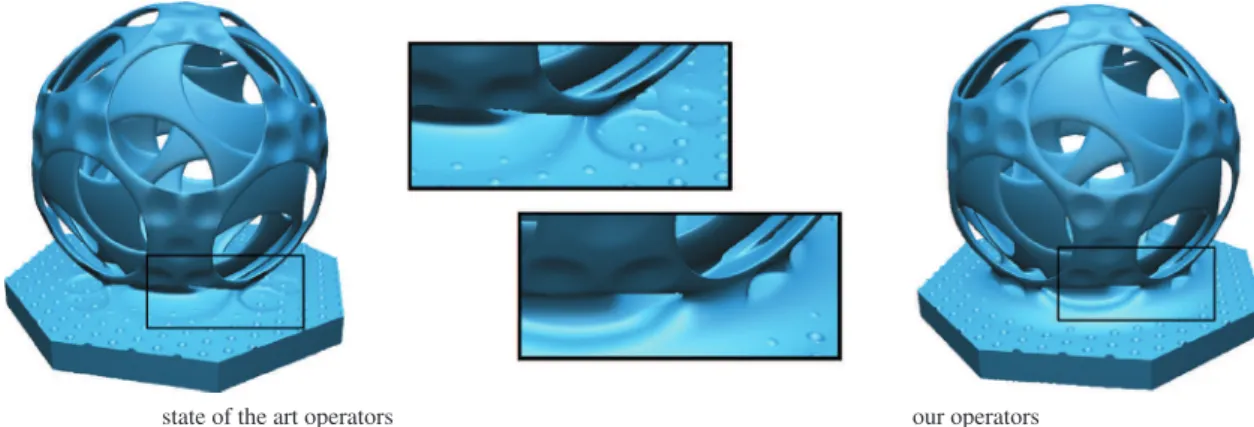
Together, our novel sets of operators allow us to safely model objects composed by unions, differences and intersections, with and without smooth transitions. This is illustrated inFig. 1where after several compositions with state of the art operators the blending shapes become uncontrollable and unsuitable while they remain controllable and as expected with our operators.
2. Related works
The simplest composition operators applying to compact field functions are the n-ary maxð:Þ and minð:Þ, which perform a Boolean union and intersection respectively [1,2]. Another well known operator is the n-ary blending operator of Ricci[2]:
gðx0…xnÞ ¼ ðx
m
0 þ ⋯ þ xmnÞ1=m; ð3Þ
where m controls the blending size. When m¼ 1, it boils down to a simple sum, as the popular operator of Blinn [3], whose contin-uous extension by Bloomenthal and Shoemake [23] yielded to convolution implicit surfaces.
While several new composition operators[24–26] and compo-sition concepts [27,28] are introduced for field functions with global support, operators for compactly supported fields received less attention until the last decade. Hsu and Lee[13]improved the control of the blending size using adequate transfer functions modifying the slope of the composed field functions. Barthe et al.
[14] defined a set of constraints for the creation of binary composition operators on compact fields, focusing on the implicit surface and the outside bound of the field functions. Based on these constraints, a new blending operator with shape control and a clean-union operator (union with a smooth field everywhere except at the surface intersections) are proposed. de Groot et al.
[15]used transfer functions to modify the field functions fiso that
when they are summed, the resulting n-ary operator is a blend in which the blending shape between the combined implicit surfaces is controlled pairwise.
Following the previous constraints[14], Bernhardt et al.[16]
introduced locally restricted binary blending operators for com-pact field functions. They can interpolate between a clean-union and a blend through a parameter used to restrict the blend where
our operators state of the art operators
Fig. 1. A complex model built (left) with Gourmel et al. gradient-based operators and (right) with our novel operators. As we can see in the zoom in the middle-top, details on the spheres consequently deform the blend between the spheres and the pedestal while in the middle-bottom our new operators preserve the blending shape. In addition, in the middle-top the same blending shape is smooth on the pedestal and unexpectedly sharp on the sphere, while in the middle-bottom it is nicely smooth on both objects with our operators.
the combined implicit surfaces intersect only. The blending size is automatically adapted to the size of the combined implicit surfaces.
Gourmel et al. [17] proposed a binary blending operator parametrized by the angle between the gradient of the composed field functions. This gradient-based operator automatically loca-lizes the blend, adapts the size of the blend to the size of the combined implicit surfaces, and avoids unwanted bulging.
In all the aforementioned approaches, no specific treatment is done for the inside part of the field functions. A marginal exception is the work of Hsu and Lee[13]where an inner bound is introduced to directly control the blending size when material is removed. In this work, this bound is not related to any operator conformity property. In summary, all these advanced binary operators exhibit the consistency problem and the lack of field variation control raised inSection 1.
3. Compactfield function representation
Before studying the composition operators in the next section, we present our consistent representation of compact fields and its properties. As we observed in Eqs.(1) and(2), the complement (1−f) of a compact field function f is composed in a union or blending operator g∪ for the definition of both intersection and difference operators. Therefore, (1−f) must satisfy all the proper-ties of compact field functions on which the definition of composi-tion operators rely: it must be positive, greater than the isovalue 0.5 inside the volume delimited by the implicit surface, and lower than 0.5 outside with decreasing values when getting further from the surface up to a bound. Outside this bound, the function (1−f) must uniformly equal zero.
This is not the case in general, but all these properties are automatically satisfied as soon as we set an inner bound to 1 in the field of f. This manipulation is simple and as shown below the different families of field functions used in geometric modeling of 3D objects can be easily adapted to satisfy this additional requirement. Special care has to be taken on the size of the band in which the field function varies. Indeed, outside this band, it is impossible for any composition operator to produce shapes that are not already part of the input surfaces. This band has to be large enough so that any such additional shape that a user would like to generate can be generated. In general, composition behaviors in inner and outer field parts are expected to be symmetric and a default solution is the generation of symmetric field functions. If required, the widths of the inner and outer bands can be set freely to accommodate for any specific constraint.
Handling global distance fields. Several families of global support field functions fgare useful for shape representation. Among them,
we can cite polynomials, radial basis functions[29,30], point set surfaces[31–33], volumetric diffusion[34,35] and others. Without lack of generality, the standard convention for them is to consider the 0-isovalue as the implicit surface where the set of points p∈R3
for which fgðpÞ o 0 defines its inner part, and the set of points for which fgðpÞ 4 0 defines its outside.
In order to benefit from all compact representation advantages, the field functions fgare composed with a transfer function tgsuch
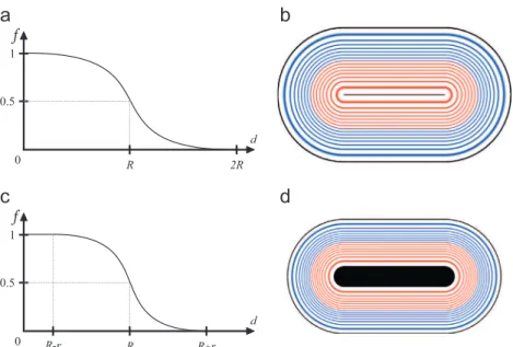
that the implicit surface is not modified but the field, inside and outside, is bounded. As depicted inFig. 2(a), we suggest defining tgas tgðxÞ ¼ φðx=rÞ where φ is a smooth-step function, and r is the
symmetric width of the band in which the resulting compact field f ¼ tg○fg
varies. This width r is defined with respect to the input field metric. For the choice of φ, any smooth-step functions, such as those proposed by Li et al.[36]and Li[26], can be selected. In this paper we used the following popular C2polynomial function
for its simplicity:
φðxÞ ¼ 1 if x ≤−1 0 if x≥1 −163x5þ5 8x3−1516x þ 0:5 otherwise: 8 > < > : ð4Þ
This mapping is symmetric, but if required, individual controls on the inner and outer widths can be achieved using, for instance, Hsu's et al. step function [13]. The use of transfer functions for similar conversions is actually common. For instance, transfer functions have also been used for adapting blending operators, that were designed for compactly supported fields, to globally supported ones[37]. In this work the conventions for global field functions are preserved and only the outside part is considered for controlling the blend.
Handling non-consistent compact distance fields. As for global support fields, any compact field function fc can be adapted to undertake our constraints by applying an adequate inner bound. For instance, fcmight come from skeleton-based soft-objects[4],
convolution surfaces[23], or objects resulting from nonconform-ing compositions[12,14]. To this end, we use the transfer function tcðxÞ ¼ φ c−x
r % &
; ð5Þ
where c is the isovalue of the implicit surface in fc
, and r∈½0; c' is the width of the symmetric band defined with respect to the input field metric. The shape of the resulting compact field f ¼ tc○fcis
shown inFig. 2(b). As for the transfer function tg, tccould easily be
adapted to offer individual control on both the inner and outer bounds.
When applied on a skeleton-based soft-object, our representa-tion results in the field funcrepresenta-tion presented inFig. 3, where R is the distance from the skeleton to the surface, and r the width of the inner and outer bands. In all our field visualizations, the inner field is colored in red and the outer one is in blue. The outer bound (where 0 ≤f oϵ) and the region inside the inner bound (where 1−ϵof ≤1) are colored in black.
4. Composition operators
Now that the field functions representing the objects to be combined are adequately defined to support the operator con-structions presented in Eqs.(1)and(2), we address the composi-tion operators. We focus on binary operators represented by functions g : R2
-R.
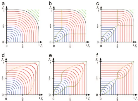
In order to better understand the way operators are built, it is convenient to consider gðf1; f2Þ as a 2Dfield function and visualize
its isocurves as in the first row ofFig. 4following the previous color code. Being of particular interest, the 0.5-isocurve is drawn in magenta and values greater than 1 are in green. In this representation, vertical (respectively horizontal) parts of isocurves
Fig. 2. (a) Function tgtransferring a global support field function from ' −∞; þ∞ ½
to our compact support field representation [0, 1] and (b) function tcadjusting the
of operator g correspond to the set of points for which gðf1; f2Þ ¼
f1 (resp. gðf1; f2Þ ¼ f2), i.e., it represents the isosurfaces of field
function f1(resp. f2).
Fig. 4shows, by column and from left to right, the max operator
resulting in a union of the implicit surfaces, a clean-union operator also implementing a union of the implicit surfaces but with a smooth field elsewhere, and a C1 blending operator which
smoothly links values of f1 to those of f2. This last operator
corresponds to Ricci's function of Eq.(3) with m¼ 2.
Following our boundary settings, an adequate operator g must satisfy several constraints. Firstly, as explained by Barthe et al.[14], it must guarantee the continuity of the field function f¼g(f1, f2) at
the support boundaries of f1 and f2. This is done by imposing g
(f1,0)¼ f1(along the abscissa axis) and with g(0, f2) ¼f2(along the
ordinate axis). In particular, g(0,0) ¼0. Equivalent constraints must now be added along the inner boundary. This is done by imposing g(f1, 1)¼ g(1, f2) ¼1. In particular, g(1, 1)¼1. In previous works,
g was only constrained to be positive on the Rþ( Rþ domain.
However, in order to keep the resulting field f consistent during
composition, any operator must now remain between the inner and outer bounds (i.e., 1 and 0 respectively). More formally this means that gðf1; f2Þ∈½0; 1' for all ðf1; f2Þ∈½0; 1'2 and g is a
function g : ½0; 1'2
-½0; 1'.
A naive way to enforce the above constraints is to take existing union or blending operators, and to clamp their value to the [0, 1] range. However, this introduces several unwanted artifacts in the resulting field f¼g(f1, f2).
Firstly, it creates gradient discontinuities in the field f along the boundary where values are clamped, regardless of the boundary continuity of the input fields. Such discontinuities prevent the use of the resulting field with operators that exhibit a low degree of continuity along their axes. For instance, this excludes the popular sum operator that would produce at most C0only surfaces, as well
as the circular blending operator of Fig. 4 that would lack curvature continuity.
Secondly, clamping the resulting field arbitrarily truncates the field at its 1-isosurface, whereas, as explained in Section 3, the width of the inner band of a field function has to be correctly set in
Fig. 3. Compact field functions defined from the distance to a linear segment skeleton. In the first row, r¼0. The field is bounded in [0, 1] and varies inside the volume up to the skeleton. In the second row, 0 o r o R. The field is a narrower band around the implicit surface and there is an inner bound within which the field function uniformly equals 1. Note that the 0.5-isosurface is the same in both cases. (For interpretation of the references to color in this figure caption, the reader is referred to the web version of this article.)
union clean-union blending
Fig. 4. Illustration of three binary composition operators. The first row shows the isocurves of the 2D scalar field of each operator, with in green the values greater than 1. The second row shows their respective effect on two spherical bounded objects. The transparent surfaces are the 0.5-isosurface of the resulting fields, and their variation is illustrated in a planar section in which the lines correspond to different isovalues. (For interpretation of the references to color in this figure caption, the reader is referred to the web version of this article.)
order to fulfill the desired modeling properties. In addition, this undesirable behavior increases with the number of overlapping compositions as shown inFig. 5.
We present two sets of operators avoiding the aforementioned problems. The adaptation of state of the art binary operators (Section
4.1) and new operators allowing us to model small details by composition without introducing field depressions (Section4.2).
4.1. State of the art binary operators
Union and blending. Among the various operators developed for compact field functions, we present the adaptation of Gourmel et al.[17]operators. These operators are the more general and the most challenging to handle. The same modification procedure can be applied to other state of the art families of binary operators such as those of Bernhardt et al.[16]and Barthe et al.[14].
As illustrated inFig. 6 top-row, Gourmel et al. [17] propose a continuous set of C∞ operators g
θ interpolating between a
clean-union and a very smooth blend according to a parameter θ. Each operator gθis built from a profile curve kθ(shown in orange) that is
symmetric with respect to the f1¼ f2diagonal. Outside this profile,
the operator simply returns the maximum of f1and f2. Inside, a blend
is realized by instancing iso-curves ρðϕÞ defined in polar coordinates. Intuitively, they mimic circular arcs but with C∞ continuity at
junctions. The set of operators is thus produced by continuously varying the profile curves kθwith respect to θ. Since this construction
does not yield closed-form formulas, operators are computed numerically and baked into 3D textures parameterized in f1; f2; θ.
As can be seen inFig. 6, these operators, as all other existing blending operators, are not bound to 1. To overcome this issue without introducing the aforementioned problems, an effective solution consists of ensuring that along the f1¼ 1 and f2¼ 1 axes,
gθð1; f2Þ ¼ gθðf1; 1Þ ¼ 1.
This is automatically achieved by designing the profile curves kθ such that they meet at f1¼ f2¼ 1, thus“closing” the blending
region of the operator as depicted inFig. 6bottom-row. To this end, we modify the boundary functions kθ as follows:
kθðf Þ ¼
kbaseθ if f ≤0:5
1 2
τðf Þ
tanhð1Þþ 1ð2− tan ðθÞÞ þ tan ðθÞ
' ( otherwise ' 8 > < > :
where τðf Þ ¼ ðtanh ○ tanh ○ tan Þðπðf −1ÞÞ, f ∈½0; 1', and kbaseθ is the
original boundary function proposed by Gourmel et al.[17]. The intuition behind the construction of these functions is the use of trigonometric and hyperbolic functions for their natural C∞
continuity and the composition for controlling the slope of there shape.
The practical effect of our new operators is depicted inFig. 7on a clean union, a blend and a gradient-based blend of two cylindrical primitives. Observe how the depression in the inner part (shown in green) is effectively removed. In the work by Gourmel et al., the parameter θ can be automatically adjusted from the angle between the gradients of f1and f2through a user defined
controller. For instance, this allows us to localize the blending effect as with the “camel” controller that has the property to remove unwanted bulge as in Fig. 7(c). Note the additional distortions introduced by this operator in Fig. 7(c)-left that are removed by our improvements inFig. 7(c)-right. This is particu-larly interesting for subsequent gradient-based compositions in which these field distortions would introduce artifacts due to unpredictable gradient variations.
Intersection and difference. We now have all the ingredients to build artifact-free intersection and difference operators by com-bining our modified union and blending operators following Eqs.
(1)and(2). The benefits of our approach are depicted inFig. 8. As we can see, the negative values (shown in yellow) produced by state of the art operators when building the cylinder in Fig. 8
(a) are avoided by our operators in Fig. 8(b). This prevents the parallelepiped from being unexpectedly deformed by the presence of negative values when it is blended with the cylinder as in Fig.8
(c) and to obtain the expect result in Fig.8(d). 4.2. Operators for details
In this section we study the application of union, blending, and difference operators when they are used to add thin details onto an existing surface. In this case, very small objects are added or removed to significantly larger ones. As shown in Fig. 9(b), classically designed operators, including the ones of the previous Section, introduce field depressions of the shape of the combined small object (a sphere in this example) where it has been added or removed. When field functions are composed, the resulting field function is expected to approximate a distance field to the implicit surface with some additional continuity and boundary constraints. The metric of this resulting field should correspond to the ones of the operands. These depressions are thus undesired from both the theoretical point of view and the practical point of view as they introduce unpredictable shape behavior when they are crossed by a blend. This is clearly illustrated in the close-up ofFig. 1(left) in which small spheres removed to deform a large one generate holes in a subsequent blend.
This leads us to the definition of a very particular operator. Indeed, when modeling small details, the resulting field is expected to progressively vary from the detailed implicit surface to the field of the large object, as shown inFig. 9(e). Assume f1is
the initial large scale field and f2 is the field of the detail. This
means that while the operator has to preserve the field properties of f1(i.e., g(f1, 0)¼ f1and g(1, f2)¼1), it must modify those of the
field f2so that it is smoothly absorbed by the field of f1. This means
that in this special case, the constraints g(0, f2)¼ f2and g(f1, 1)¼1
do not have to be respected for f240:5. To achieve this behavior, we have to build a new set of gradient-based operators ~gθ that
reproduce gθin the outer part of both field functions f1and f2, and
which progressively reproduce the field of f1when moving away
from the 0.5 isovalue of operator gθ.
In our representation of binary composition operators (Fig. 10), this means that the operator ~gθ must be a standard blending
Fig. 5. Intersecting 2 planes (first row) and composing 4 cylinders to build a star (second row) using a clamped version of the clean union operator (a) leads to uncontrollable bound cutting, while with our operators (b) the bounds of the planes and cylinders are preserved.
operator for ~gθo0:5. Outside this region, isocurves of ~gθ must
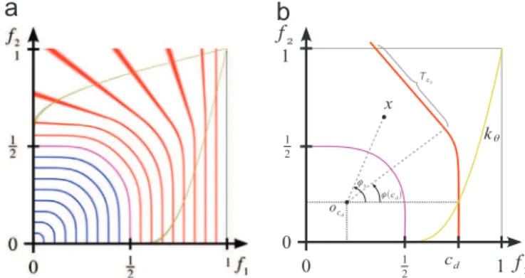
smoothly vary for increasing isovalues to become a straight vertical line at f1¼ 1. This operator is depicted inFig. 10(a).
Our first attempt to design such an operator was to simply perform a linear interpolation between gθ and f1 according to a
parameter αðf1; f2Þ. However, designing α to obtain the expected
operator appeared to be very challenging. Instead, we propose to precisely define the shape of each individual isocurve of ~gθusing
the following construction.
We define the isocurves of the detail operator ~gθby modifying
the ones of gθ that are greater than 0.5 such that they become
straight at an angle ϕð ~gθÞ in a local polar coordinate system as
depicted by the red curve inFig. 10(b). When ϕ ¼ π=2 we exactly reproduce gθ, and when ϕ ¼ 0 we obtain the straight vertical
Fig. 6. Top-row, the state of the art gradient-based blending operators[17]produce values greater than one (green part). These operators are constructed from yellow boundary curves kθdetermining the blending radius of the operator isovalues. Three different values of θ are shown with (a) full blending, (b) intermediate blending, and
(c) clean-union. Bottom-row shows our respective “closed” versions of these operators. (For interpretation of the references to color in this figure caption, the reader is referred to the web version of this article.)
state of the art operators our operators
Fig. 7. Closing the boundary functions of a gradient-based blending operator leads to better shaped resulting potential fields. Applying previous operators (left) and our operators (right) using (a) clean union, (b) blending and (c) “camel” blending.
state of the art ours
Fig. 8. Top row: a hollow cylinder is built by removing a cylinder from another larger and then intersecting with 2 planes. The use of Gourmel's operators[17]on the left produces negative field values that lead to an inadequate deformation of the blended cuboid on its side, where pointed in (c) by the red arrows. This misbehavior is naturally avoided by the use of our operators as shown in (d). (For interpretation of the references to color in this figure caption, the reader is referred to the web version of this article.)
isocurves reproducing f1. Then, ϕ smoothly varies between π=2 and
0 when ~gθvaries from 0.5 to 1 as
ϕðtÞ ¼ π 2ð2−2tÞ
s: ð6Þ
Here the exponent s adjusts the interpolation speed between the 0.5-isovalue and the field f1.
As for gθ in Gourmel et al.[17], this definition of ~gθ does not
allow its analytical evaluation. It is evaluated as follows. Given a point x ¼ ðf1; f2Þ, c ¼ ~gθðxÞ is the value we want to compute. In this
explanation, we follow the illustration ofFig. 10(b). If x is below the 0.5-isocurve of gθ shown in magenta (i.e., gθðxÞ ≤0:5) then
c ¼ gθðxÞ. Likewise, if x is below the profile curve kθ shown in
yellow (i.e., f2okθðf1Þ) then, by construction, c ¼ f1. Otherwise c is numerically evaluated with a dichotomic search in the range [0.5, 1], starting with cd¼ 0.75 as the initial guess. If x is below the cd-isocurve
shown in red, we continue the search within the range [0.5, cd].
Otherwise, we continue the search within the range [cd, 1]. To
determine the position of x with respect to the cd-isocurve, we
express its position in polar coordinates ðϕx; ρxÞ in the local frame
centered at ocd¼ ðkθðcdÞ; kθðcdÞÞ. Then three cases occur:
$
If ϕx≤ 0, then x is below the cd-isocurve.$
If ϕx≤ ϕðcdÞ, x is below the cd-isocurve if ρðϕxÞ o ρx, where ρðϕÞis the profile curve used to define the blending operator gθ.
$
Otherwise we directly check whether x is above or below the tangential half-line Tcd.As for gθ, this operator is precomputed into a 3D grid, and its
gradients are computed by means of finite differences. Note that
precomputations in grids are easier to perform as the range of evaluation for (f1, f2) is now restricted to [0, 1]2.
This operator is illustrated inFig. 9for different values of the parameter s which modulates the absorption of the blended/ subtracted field. In practice, we suggest using s¼4 which has been used for all the examples in this paper.
5. Results and discussions
The precomputation of our operator with inner and outer bounds and its partial derivatives in 1283grids takes about 0.9 s
on a Core I7 950. The same precomputations for our detail-specific operator take about 9 s. Their transfer from the host memory to the device memory as 3D textures takes 3 ms. The evaluation of any operator stored in 3D textures boils down to a single texture fetch and the evaluation cost is thus irrespective to its actual equation complexity. This explains why our operators achieve the same performance as previous gradient based operators[17]. On a NVIDIA GTX 480, 100 million evaluations are done in less than 35 ms.
Using both our compact support field representation and our new operators, we can now design complex objects with adequate field variations and metrics in there inside part. These objects can be drilled with a guaranty that the resulting object is well shaped.
Fig. 1illustrates a complex object built with several differences and blends. As we can see on the left ofFig. 1, despite all there nice properties, Gourmel et al. operators fail in preserving field varia-tions and metrics when several differences are used. The field of the large drilled spheres has been altered and a consequence is the asymmetry in the blend between the large spheres and the pedestal. As shown in the right ofFig. 1, the use of our operators prevent these alterations of the field and the blend is symmetric. When making a difference operation, a very interesting obser-vation is that the inner field of the subtracted primitive defines a part of the outer field of the result. Another important observation is that after a composition, we expect the resulting field to follow the shape of the resulting surface as if approximating the varia-tions of a distance field. Without inner field control, this is not the case in the inner field part when clean union and blending are used as illustrated in Fig. 7where unexpected field depressions arise. The use of an inner bound together with the adapted operators avoid this problem. This is also usually not the case for the difference. Reducing the inner radius of the combined objects enables the generation of a band around the implicit surface, as for
Fig. 9. (a) A parallelepiped on which a sphere has been added (blending) and a sphere has been removed (difference with smooth transition). While this surface is the same for all operators, the resulting field has different local variations where the spheres are combined. This is illustrated in the planar section of the resulting field function passing by the middle of the added and removed spheres. (b) State of the art operators create field depressions. Our new detail operator (c)–(f) absorbs the blended/subtracted field functions. As we can see, the absorption is modulated by the parameter s.
Fig. 10. (a) Illustration of our asymmetric operator for details ~gθ with θ ¼ 0 and
s¼ 1. (b) Illustration of the construction of this operator. The cd-isocurve shown in
red is obtained by cutting the original isocurve of gθat a polar angle ϕðcdÞ and
prolonging it by a straight line Tcd. The evaluation of ~gθat an arbitrary position x is
performed by iteratively determining whether x is above or below the isocurve of the current guess cd. The profile curve kθis shown in yellow, and the 0.5-isocurve in
magenta. (For interpretation of the references to color in this figure caption, the reader is referred to the web version of this article.)
the tubes in Fig. 11 (top-row). In this band, the field smoothly approximates a distance field with the metric of the composed field functions.Fig. 11(bottom-row) shows a similar control on a capsule subtracted from a sphere.
Whereas symmetric operators are well suited for large-scale compositions (Section 4.1), when modeling small features, our detail-aware operator becomes preferable (Section 4.2). This is demonstrated inFig. 12where a golf-ball like shape is obtained by removing small spheres from a large one, and then blending the result with a pedestal. Using symmetric difference operators, the depressions introduced in the field when removing the small spheres (Fig. 12(a)-bottom) distort the blend between the ball and
the pedestal (Fig. 12(a)-top). This behavior is undesired and unexpected as these small spheres just represent a detail and the blend should mostly be as the one linking the ball (a large sphere) and the pedestal. Fig. 12(b) illustrates the improvement obtained by using our new detail specific operator. These beha-viors are also illustrated inFigs. 1and13.Fig. 13also illustrates the field variations generated when objects are built using our compact field representation together with our composition operators.
6. Conclusion
In this paper we have presented new constraints on field functions so that intersection and difference composition opera-tors are applied in a consistent manner, avoiding field distortions and discontinuities. We also provide a method to build composi-tion operators satisfying those constraints when interseccomposi-tion and difference operators are derived from union or blending. Combin-ing these contributions allows, when applyCombin-ing difference opera-tors, to dig the outer bound of the resulting field function so that its shape follows the shape of the surface.
Finally, we have introduced a new specific composition opera-tor for the modeling of thin details on a surface. This operaopera-tor
Fig. 11. Adjusting the external boundary using the inner bound and subtracting field functions. Top row: (a) a cylinder is removed from a slightly larger one. Intersection with planes are used to get the final result in (b). Bottom row: (c) a capsule is removed from a sphere. Observe in (b) and (d) how the field approximates a smooth distance field around the implicit surfaces.
Fig. 12. Illustration of our new operator for details. (a) The details are created using our difference operator and (b) using our new detail-specific difference operator. Note the field depressions introduced in (a)-bottom and the resulting blend deformation between the ball and the pedestal (a)-top that are avoided in (b) with our detail-specific operator.
Fig. 13. A flute model built using our compact field functions and our adapted composition operators including detail-specific operators. The quality of the field variations is illustrated on a vertical section of the left side of the field function. Note that unexpected depressions are avoided and the field approximates a distance field in bands located on each side of the implicit surface.
smoothly absorbs the removed field, thus avoiding the introduc-tion of undesired depressions in the resulting field funcintroduc-tion that would degrade the shape of subsequent smooth transitions.
These advanced operators do not yield analytic formulas and have to be precomputed into tables to enable fast evaluations. As future work, it might be interesting to derive analytic formulas reproducing our operators, even if that means losing C∞continuity.
This paper highlights the importance of the quality and shape of both the inside and outside fields. In the context of an interactive modeling system, these observations yield interesting questions such as how to leverage a maximal control on the resulting fields? The study of interactive visualizations, especially for the creation of small details and field function based micro geometries would also be of interest. Finally, the way the details could be positioned and repeated on the surface is another direction to investigate.
Acknowledgments
This work has been funded by the IM&M project (ANR-11-JS02-007).
References
[1] Sabin MA. The use of potential surfaces for numerical geometry. Technical Report VTO/MS/153, British Aerospace Corp., Weybridge, UK; 1968. [2]Ricci A. A constructive geometry for computer graphics. Comp J 1973;16
(2):157–60.
[3]Blinn JF. A generalization of algebraic surface drawing. ACM Trans Graph 1982;1(3):235–56.
[4]Wyvill G, McPheeters C, Wyvill B. Data structure for soft objects. Vis Comp 1986;2(4):227–34.
[5] Bloomenthal J. Bulge elimination in convolution surfaces. Comp Graph Forum 1997;16:31–41.
[6]Shapiro V. Semi-analytic geometry with R-functions. Acta Numer 2007;16: 239–303.
[7]Olsen L, Samavati FF, Sousa MC, Jorge JA. Technical section: sketch-based modeling—a survey. Comput Graph 2009;33(1):85–103.
[8] Brazil EV, Macedo I, Sousa MC, de Figueiredo LH, Velho L. Sketching variational hermite-RBF implicits. In: Proceedings of the seventh sketch-based interfaces and modeling symposium (SBIM ’10); 2010. p. 1–8.
[9]Galin E, Akkouche S. Incremental polygonization of implicit surfaces. Graph Models 2000;62(1):19–39.
[10]Kanamori Y, Szego Z, Nishita T. GPU-based fast ray casting for a large number of metaballs. Comput Graph Forum 2008;27(2):351–60.
[11]Gourmel O, Pajot A, Paulin M, Barthe L, Poulin P. Fitted BVH for fast raytracing of metaballs. Comp Graph Forum 2010;29(2):281–8.
[12]Wyvill B, Guy A, Galin E. Extending the CSG tree – warping, blending and boolean operations in an implicit surface modeling system. Comput Graph Forum 1999;18(2):149–58.
[13]Hsu PC, Lee C. Field functions for blending range controls on soft objects. Proceedings of Eurographics. Computer Graphics Forum 2003;22(3):233–42. [14]Barthe L, Wyvill B, de Groot E. Controllable binary CSG operators for “soft
objects”. Int J Shape Model 2004;10(2):135–54.
[15]de Groot E, Wyvill B, van de Wetering H. Locally restricted blending of blobtrees. Comput Graph 2009;33(6):690–7.
[16]Bernhardt A, Barthe L, Cani MP, Wyvill B. Implicit blending revisited. Proceedings of Eurographics. Comp Graph Forum 2010;29(2):367–76. [17]Gourmel O, Barthe L, Cani MP, Wyvill B, Bernhardt A, Paulin M, et al. A
gradient-based implicit blend. ACM Trans Graph 2013;32(2).
[18]Barthe L, Mora B, Dodgson N, Sabin M. Interactive implicit modelling based on C1 reconstruction of regular grids. Int J Shape Model 2002;8(2):99–117. [19]Ferley E, Cani MP, Gascuel JD. Resolution adaptive volume sculpting. Graph
Models 2002;63:459–78.
[20] Schmitt R, Wyvill B, Galin E. Interactive implicit modeling with hierarchical spatial caching. In: Shape modelling international; 2005.
[21] Eyiyurekli M, Breen DE. Data structures for interactive high resolution level-set surface editing. In: Proceedings of graphics interface 2011 (GI’11); 2011. p. 95–102.
[22]Brun E, Guittet A, Gibou F. A local level-set method using a hash table data structure. J Comput Phys 2012;231(6):2528–36.
[23]Bloomenthal J, Shoemake K. Convolution surfaces. SIGGRAPH Comput Graph 1991;25(4):251–6.
[24]Pasko A, Adzhiev V, Sourin A, Savchenko V. Function representation in geometric modeling: concepts, implementation and applications. Vis Comp 1995;11(8):429–46.
[25]Barthe L, Gaildrat V, Caubet R. Extrusion of 1D implicit profiles: theory and first application. Int J Shape Model 2001;7:179–99.
[26]Li Q. Smooth piecewise polynomial blending operations for implicit shapes. Comput Graph Forum 2007;26(2):157–71.
[27]Barthe L, Dodgson NA, Sabin MA, Wyvill B, Gaildrat V. Two-dimensional potential fields for advanced implicit modeling operators. Comp Graph Forum 2003;22(1):23–33.
[28]Pasko GI, Pasko AA, Kunii TL. Bounded blending for function-based shape modeling. IEEE Comput Graph Appl 2005;25(2):36–45.
[29] Carr JC, Beatson RK, Cherrie JB, Mitchell TJ, Fright WR, McCallum BC, et al., Reconstruction and representation of 3d objects with radial basis functions. In: Proceedings of the 28th annual conference on computer graphics and interactive techniques (SIGGRAPH ’01). ACM; 2001. p. 67–76.
[30]Macêdo I, Gois JP, Velho L. Hermite radial basis functions implicits. Comp Graph Forum 2011;30(1):27–42.
[31] Adamson A, Alexa M. Approximating and intersecting surfaces from points. In: Kobbelt L, Schröder P, Hoppe H, Proceedings of the Eurographics Symposium on Geometry Processing, vol. 23; 2003. p. 245–54.
[32]Shen C, O'Brien JF, Shewchuk JR. Interpolating and approximating implicit surfaces from polygon soup. ACM Trans Graph 2004;23(3):896–904. [33] Guennebaud G, Gross M. Algebraic point set surfaces. In: ACM SIGGRAPH 2007
papers (SIGGRAPH ’07). New York, NY, USA: ACM; 2007.
[34] Davis J, Marschner SR, Garr M, Levoy M. Filling holes in complex surfaces using volumetric diffusion, In: 3D data processing visualization and transmis-sion. IEEE Computer Society; 2002. p. 428–38.
[35]Calakli F, Taubin G. SSD: smooth signed distance surface reconstruction. Comput Graph Forum 2011;30(7):1993–2002.
[36] Li Q, Phillips R. Implicit curve and surface design using smooth unit step functions. In: Proceedings of ACM symposium on solid modeling and applications (SM ’04). Eurographics Association; 2004. p. 237–42.
[37] Barthe L, Gaildrat V, Caubet R. Combining implicit surfaces with soft blending in a CSG tree. In: Proceedings of the CSG conference series; 1998. p. 17–31.