UNIVERSITÉ DU QUÉBEC
ÀMONTRÉAL
THE SENSITIVITY OF REGIONAL CLIMATE
SIMULATIONS TO DOMAIN SIZE AND LARGE SCALE
DRIVING TECHNIQUE
DISSERTATION PRESENTED
AS PARTIAL REQUIREMENT
FOR MASTER'S DEGREE IN ATMOSPHERIC SCIENCE
BY
DRAGANA KORNIC
UNIVERSITÉ DU QUÉBEC À MONTRÉAL Service des bibliothèques
Avertissement
La diffusion de ce mémoire se fait dans le respect des droits de son auteur, qui a signé le formulaire Autorisation de reproduire et de diffuser un travail de recherche de cycles
supérieurs (SDU-522 - Rév.01-2006). Cette autorisation stipule que «conformément
à
l'article 11 du Règlement no 8 des études de cycles supérieurs, [l'auteur] concède
à
l'Université du Québecà
Montréal une licence non exclusive d'utilisation et de publication de la totalité ou d'une partie importante de [son] travail de recherche pour des fins pédagogiques et non commerciales. Plus précisément, [l'auteur] autorise l'Université du Québec à Montréal à reproduire, diffuser, prêter, distribuer ou vendre des copies de [son] travail de rechercheà
des fins non commerciales sur quelque support que ce soit, y compris l'Internet. Cette licence et cette autorisation n'entraînent pas une renonciation de [la] part [de l'auteur]à
[ses] droits moraux nià
[ses] droits de propriété intellectuelle. Sauf entente contraire, [l'auteur] conserve la liberté de diffuser et de commercialiser ou non ce travail dont [il] possède un exemplaire.»UNIVERSITÉ DU QUÉBEC
ÀMONTRÉAL
SENSIBILITÉ DES SIMULATIONS DU MODÈLE
RÉGIONAL DU CLIMAT
À
LA TAILLE DU DOMAINE
ET
À
LA TECHNIQUE DE PILOTAGE
MÉMOIRE PRÉSENTÉ
COMME EXIGENCE PARTIELLE
DE LA MAÎTRISE EN SCIENCES DE L'ATMOSPHÈRE
PAR
DRAGANA KORNIC
RENlERCIEMENTS
Premièrement, je voudrais remercier mon directeur de recherche, le Dr. René Laprise, pour ses conseils scientifiques et son inspiration jusqu'à la fin de mon mémoire, Martin Leduc, pour ses nombreuses suggestions, le Centre ESCER, pour le soutien financier pendant mes études de maîtrise, ainsi que tout le personnel de département de sciences de l'atmosphère de l'Université du Québec à Montréal. Enfin, je voudrais remercier ma famille pour le soutien moral et leur encouragement, malgré la distance.
TABLE DES MATIÈRES
LISTE DES ACRONYMES vii
LISTE DES SYMBOLES viii
RÉSUlVJÉ ix
INTRODUCTION 1
CHAPITRE 1
SENSIBILITÉ DES SIMULATIONS DU MODÈLE RÉGIONAL DU CLIMAT À LA TAILLE DU DOMAINE ET À LA TECHNIQUE DE PILOTAGE 5
Abstract 7
1. Introduction 8
2. Model description Il
3. Experimental setup 12
3.1 Domain-size sensitivity (BB protocol) 12
3.2 Sensitivity experiment nesting technique 13
3.3 Statistical analysis 15 4. Results 17 4.1 Total fields 17 4.2 Small scales 19 4.3 Taylor diagrams 21 5. Conclusion 23 BIBLIOGRAPHIE 26 FIGURES 29 CONCLUSION 42
LISTE DES FIGURES
Figure
Page
Schematics of the Big-Brother (BB) experimental protocol a The BB high-resolution simulation with the area of interest (dashed line) b The BB solution after using the low-pass filter c The Little-Brother (LB)
high-resolution simulation 30
2 The computational domains of the Big Brother (BB: 196x196 grid points) and
the Little Brothers (LB 1 to LBS) having respectively 196x 196, 160x 160, 140x140, 120x 120 and 1OOx 100 grid points. The climate statistics are verified
through the QC area (dashed) of 86x86 grid points 31
3 Spatial correlation of LB with BB for the stationary (left side column) and transient-eddy standard deviation (right side column), as a function of LB domain size and SN strength: a 925hPa temperature b 700hPa relative hurnidity c precipitation d 500hPa relative vorticity 32 4 Stationary component of the precipitation rate field for the LBs a 120 b
160 and c 196 for the different experiments with
1
no SNII
0-5% SN andIII
50/0 SN 33S Transient component of the precipitation rate field for the LBs a 120 b 160 and c 196 for the different experiments with 1no SN
II
0-5% SN andIII
5% SN 346 Spatial correlation of LB with BB for the small-scale stationary (left side colUI1U1) and transient-eddy standard deviation (right side column), as a function of LB domain size and SN strength: a 925hPa temperature b 700hPa relative humidity c precipitation d 500hPa relative vorticity 35 7 Small-scale stationary component of the 700hPa relative humidity field
for the LBs a 120 b 160 and c 196 for the different experiments with 1 no
VI
8 Small-scale transient component of the 700hPa relative humidity field for the LBs a 120 b 160 and c 196 for the different experiments with 1 no SN
II 0-5% SN and III 5% SN 37
9 Small-scale stationary component of the precipitation field for the LBs a 120 b 160 and c 196 for the different experiments with 1 no SN II 0-5%
SN and III 50/0 SN 38
10 Small-scale transient component of the precipitation field for the LBs a 120 b 160 and c 196 for the different experiments with 1 no SN II 0-5%
SN and III 5% SN 39
11 Taylor diagrams for the transient-eddy large-scale component of a precipitation rate, b 925hPa temperature, c 700hPa relative humidity and d 500hPa relative vorticity fields, for different experiments 40 12 Taylor diagrams for the transient-eddy small-scale component of a
precipitation rate, b 925hPa temperature, c 700hPa relative humidity and d 500hPa relative vorticity fields, for different experiments 41
AMlP BB BBE CFCAS CFL CRCM CRCMD DCT FBB GCM GF LB LBC MCG MRC MRCC NCEP NO SN pcp PF RCM rhum rv SN temp UQAM
LISTE DES ACRONYMES
Atmospheric Model Intercomparison Project Big Brother
Big Brother Experiment
Canadian Foundation for Climate and Atmospheric Sciences Conditions aux Frontières Latérales
Canadian Regional Climate Model
Canadian Network for Regional Climate Modelling and diagnostics Discrete Cosine Transform
Filtered Big Brother Global Climate Model Grand-Frère
Little Brother
Lateral Boundary Conditions Modèle Climatique Global Modèle Régional du Climat
Modèle Régional Canadien du Climat
National Centers for Environmental Prediction No Spectral Nudging
preci pitation Petit-Frère
Regional Climate Model relative humidity relative vorticity Spectral Nudging temperature
LISTE DES SYMBOLES
BB Big Brother
Kmn Nudging coefficient L Model operator Lü Lowest model level LB Little Brother
m Wave number
n Wave number
p Pressure
Q Prognostic variable
Qü Prognostic variable for driving fields Qmn Spectral coefficient for prognostic variable
QÜmn Spectral coefficient for prognostic variable for driving fields
R' Temporal correlation coefficient R
*
Spatial correlation coefficienta
Strength of spectral nudginga
max Maximal strength of spectral nudgingcp
Meteorological fieldcp
Mean part of the meteorological fieldcp'
Time deviation of the meteorological field If Meteorological fieldRÉSUMÉ
La sensibilité du Modèle Régional Canadien du Climat (MRCC) à la taille du domaine et à la technique de pilotage spectral (SN) est étudiée. Nous savons déjà que le domaine d'intégration du MRCC doit être suffisamment grand pour permettre le développement complet des petites échelles. Si l'intégration est réalisée sur un très grand domaine, elle conduit à d'importantes déviations, à moins qu'un pi 1otage des grandes échelles soit appliqué. La technique du pilotage spectral consiste à forcer les grandes échelles pas seulement aux frontières latérales, mais aussi à J'intérieur du domaine d'intégration.
L'influence des différentes tailles de domaines et l'intensité du pilotage de grande échelle est étudiée avec le cadre expérimental du « Grand-Frère». Elle consiste premièrement à établir une simulation de référence, nommée
«
Grand-Frère », GF, sur un grand domaine en haute résolution (~45km). Cette simulation est ensuite filtrée en enlevant les petites échelles. Les données résultantes (grandes échelles : ~2l60km) sont utilisées pour piloter le même modèle, intégré à la même haute résolution, mais sur un domaine plus petit issu que le domaine BB (appelé « Petit-Frère », PF). Nous avons effectué 5 simulations de PF avec 196x 196, 160x160, 140x140, 120x 120 et 1OOx 100 points de grille. Les statistiques du climat entre les simulations de GF et celles de PF sont comparées sur un domaine commun de 86x86 points de grille. Trois expériences sont réalisées: deux avec différentes intensités de pilotage (0 à 5%; 5%) et une sans le pilotage spectral.Avec l'application du pilotage de grande échelle, on note l'augmentation de la corrélation spatiale entre les simulations de PF et leur référence avec l'augmentation de la taille du domaine. Pour chaque étude, les diagrammes de Taylor montrent l'augmentation de la corrélation temporelle des caractéristiques à petites échelles, de quelques dizaines de pourcentages pour les plus grands domaines, avec les valeurs les plus hautes du coefficient de pilotage.
INTRODUCTION
Le système climatique mondial est très complexe. Afin de le comprendre, les Modèles Climatiques Globaux (MCGs) ont été développés pour simuler les caractéristiques physiques et dynamiques du système climatique.
En raison de la complexité et de la couverture mondiale, les simulations des MCGs ont un coût de calcul élevé. Les premiers MCGs ont été conçus avec une résolution très grossière, ce qui a eu pour conséquence de limiter la reproduction du climat à l'échelle régionale. Avec l'évolution des ordinateurs, les MCGs se sont améliorés. Bien que leur résolution ait été augmentée, ils sont restés limités en raison de leur incapacité
à
résoudre l'hétérogénéité de surface, la topographie et les caractéristiques des petites échelles dans l'écoulement. Ils ne ressoudent que la grande échelle et les caractéristiques de l'atmosphèreà
l'échelle synoptique. Afin de fournir des simulations à haute résolution, une technique d'emboîtement d'un Modèle Climatique Régional (MRC) a été élaborée. Cette idée a été initialement proposée par Dickinson et al. (1997) et Giorgi (1990). Elle est basée sur un concept de pilotage unidirectionnel dans lequel les champs météorologiques à grande échelle, issus des simulations MCG, fournissent des conditions initiales et les conditions aux frontières latérales (CFL) pour le modèle de haute résolution à aire limitée. Une technique de pilotage unidirectionnel a été proposée par Davies (1976), où les variables du modèle sont relaxées progressivement sur une zone éponge le long des frontières latérales.2
Lorsque la technique de pilotage est employée pour la recherche climatique, elle est nommée le raffinement dynamique (von Storch et al. 1993). L'objectif principal des !ViRC dans les études climatiques est d'ajouter les détails de la petite échelleà
la solution, mais en gardant la circulation de grande échelle du modèle mondial (e.g., Laprise, 2008).Pour qu'un MRC simule correctement le climat régional, on doit atteindre un état d'équilibre entre les informations fournies par les CFL et la physique et la dynamique du MRC. Le temps nécessaire pour parvenir à cet équilibre s'appelle le temps d'ajustement du modèle
(spin-up
en anglais). Il dépend de la taille du domaine, de la saison et de la circulation atmosphérique. Habituellement, la durée de spin-up est de quelques jours. Ainsi, on peut noter qu'un modèle à aire limitée est exécuté en mode climat lorsque la durée de la simulation dépasse le spin-up.L'incompatibilité de la physique des deux modèles (MRC et MCG) peut aussi influencer la solution du MRC. C'est pourquoi deux approches sont utilisées pour aborder cette question. Dans la première approche, les dOMées du pilote sont issues de plusieurs MCG ou de doMées de réanalyses. Dans la deuxième approche, toute la physique du modèle pilote est utilisée dans le modèle piloté. Cette dernière est utilisée dans la présente étude.
La différence de résolution entre le MRC et le MCG peut produire des circulations erronées. Trois critères doivent êtres respectés pour le choix de la résolution du MRC (Giorgi et Mearns, 1999). Tout d'abord, la résolution doit être assez fine pour prendre en compte les échelles d'intérêt (zones côtières, la topographie, etc.); ensuite, la résolution doit fournir le maximum d'informations sur la région d'intérêt; enfin, il doit être capable de capturer des échelles pertinentes de l'écoulement.
3
La taille du domaine est importante aussi dans la production de solution adéquate. Le domaine doit être suffisamment grand pour permettre le développement complet de la petite échelle, mais pas trop large parce qu'il peut développer une circulation de grande échelle différente de celle des données pilotes. Miguez-Macho et al. (2004) ont montré que les elTeurs dans la position du patron de la précipitation étaient largement dues à une déformation systématique de la circulation à grande échelle causée par son interaction avec la condition frontière latérale. Le modèle produit des biais dans la représentation des grandes échelles, puisque les ondes longues sont sensibles aux frontières latérales en tout point du domaine. Ainsi, la modélisation du climat à l'échelle régionale pose un problème de conditions aux frontières latérales contrairement à la prévision météorologique qui pose un problème de conditions initiales.Plusieurs auteurs ont suggéré la technique de pilotage spectral (spectral nudging en anglais; SN) pour résoudre le problème de dépendance de la solution à la
taille du domaine (Waldron et al., 1996; von Storch et al., 2000; Miguez-Macho et al., 2004; Laprise, 2008; Alexandru et al., 2009). La technique de SN est basée sur un point de vue dans lequel les détails des petites échelles sont le résultat d'interactions entre l'écoulement atmosphérique de grande échelle et les caractéristiques géographiques des plus petites échelles, telles que la topographie, la distribution telTe mer, ou l'utilisation des telTains (von Storch et al., 2000). Le forçage des grandes échelles n'est pas seulement aux frontières latérales mais aussi à l'intérieur du domaine. Les petites échelles sont déterminées par le MRC. Il a été noté par Laprise (2008) que le pilotage des grandes échelles doit être considéré comme une fermeture nécessaire pour les grandes échelles afin de prendre en compte une taille de domaine déterminée du MRC. L'inconvénient de la technique de SN est de masquer les elTeurs systématiques d'un MRC.
4
À cause des problèmes qui peuvent influencer le changement d'échelle d'un MRC, Denis et al. (2üü2a) ont proposé une méthode en investiguant la technique de pilotage et de raffinement dynamique. Cette méthode, nommée le cadre expérimental du
«
Grand-Frère»,
est basée sur une approche de«
pronostic parfait».
En premier lieu, le climat de référence est établi en réalisant une simulation de haute résolution sur un grand domaine, appelé«
Grand-Frère»,
GF. La deuxième étape consiste ensuite à filtrer les petites échelles du résultat obtenu. Cette référence filtrée est ensuite utilisée pour le pilotage du même MRC qui possède la même haute résolution que la référence GF mais sur un plus petit domaine, appelé«
Petit-Frère»,
PF, inclus dans le domaine GF. Les statistiques de climat de GF et PF sont donc comparées sur un domaine commun. Les différences entre eux peuvent être attribuées aux erreurs associées au raffinement dynamique et la technique de pilotage.Dans cette étude, nous utilisons l'approche de
«
pronostic parfait»
pour investiguer l'influence des différentes tailles de domaine ainsi que celles du pilotage de grande échelle (SN technique). Le MRC Canadien a été intégré sur le continent nord américain, avec une résolution horizontale de 45km. Trois configurations expérimentales différentes ont été utilisées avec 5 tailles de domaine différentes:une sans technique SN
deux avec différents profils de SN
Le mémoire est organisé de la façon suivante. Le Chapitre l constitue le travail principal du mémoire et il est présenté sous la fonne d'un article en anglais, qui sera soumis
à
la revueClimate Dynamics.
La dernière partie de mémoire consiste en une conclusion et discussion des résultats.CHAPITRE 1
SENSIBILITÉ DES SIMULATIONS DU MODÈLE
RÉGIONAL DU CLIMAT
À
LA TAILLE DU DOMAINE
ET
À
LA TECHNIQUE DE PILOTAGE
Le présent chapitre décrit brièvement le Modèle Régional Canadien du Climat utilisé dans cette étude. Ensuite, les méthodologies du cadre expérimental
«
Grand Frère» et de la technique de pilotage spectral sont présentées, ainsi que les statistiques employées et le diagramme de Taylor. Les résultats et la discussion sont présentés dans la partie centrale du chapitre. La sensibilité du MRCC à la taille du domaine et au forçage des grandes échelles est étudiée et discutée. La conclusion de cette étude finira cette section.Comme mentionné dans l'introduction, ce chapitre est présenté sous fonne d'un article rédigé an anglais qui sera soumis au journal
«
Cfimate Dynamics». La liste des Figures se trouve au début de ce mémoire. Les références de l'article et du mémoire sont insérées à la fin de l'article.The Sensitivity of Regional Climate
Simulations to Domain Size and Large-Scale
Driving Technique
Dragana Kornic, René Laprise,
and Martin Leduc
Centre ESCER (Étude et Simulation du Climat à l'Échelle Régionale) Canadian Networkfor Regional Climate Modelling and Diagnostics (CRCMD)
Département des sciences de la Terre et de l'Atmosphère Université du Québec à Montréal, Montréal, Québec, Canada
Corresponding author address: Dragana Kornic
Département des Sciences de la Terre et de l'Atmosphère, UQAM P. o. Box 8888, Stn Downtown
Montréal, Québec, Canada H3C 3P8 Tel: +] 514928-2029
7
Abstract
The sensitivity of the Canadian Regional Climate Model (CRCM) to domain size and large-scale spectral nudging (SN) is studied. It is known that the domain of integration of an RCM must be large enough to allow the full development of the small-scale features. If the integration is performed on very large domain, it shows important departures from the driving data unless large-scale driving is applied. The nudging technique consists in forcing the large scales not only at the lateral boundaries but also within the domain of integration.
The influence of different domain sizes and the intensity of large-scale driving (nudging) are studied here by using the 'perfect model' approach, nicknamed the Big-Brother Experiment (BBE). It consists in first establishing a reference simulation, named Big-Brother (BB) simulation, over a large domain of integration. This simulation is then degraded by removing the small scales. The remaining data are used to drive the same CRCM, integrated at the same high resolution but over a smaller domain embedded in the BB domain (the Little-Brother simulation). Climate statistics of both BB and LB are compared over a common area. Three experiments were performed: two experiments with different nudging intensity and one without spectral nudging, over five different domain sizes.
With the increase of large-scale nudging intensity we note an increase of spatial correlation between the simulation and their reference with larger domain sizes. Taylor diagrams for each study show the increase in temporal correlation of small-scale features of few tenths of percents for the largest domains with the stronger nudging.
8
1.
IntroductionCoupled Global Climate Models (GCMs) constitute the most advanced tools to study the physical processes that contribute to maintaining the climate equilibrium and making projections of its evolution as a result from changes in externaJ forcing. Their high computational cost however forces the use of low resolution, which can lead to errors in the regional aspects of the simulated climate. Typical resolutions of operational GCM are -25ûkm, which is insufficient for most climate-change impact studies that require scales of the order of tens of km. ln an attempt to satisfy this need for information at finer scales, the approach of'downscaling' the output from a coarser resolution GCM has gained interest.
The most common procedure for producing high-resolution numerical simulations over a region of interest is to nest a regional model within a coarser global mode!. Regional Climate Models (RCMs) get their large-scale information from the coarse-resolution global model and add finer scale details that constitute the primary potential added value of an RCM. This process works due to the fact that, by having higher resolution than GCM, RCM can resolve physical processes responsible for the generation of fine-scale details in the simulation. The use of high-resolution for RCMs is computationally more affordable than high-resolution GCM simulations because of the use of a limited-area computational domain for RCM. There remain, however, several issues related to the use of RCM, such as the impact of one-way interaction with the driving data, the nesting technique, and the RCMs' skill at generating fine-scale details from low-resolution driving data.
ln order to evaluate the downscaling skill of one-way nested RCMs, the Canadian RCM group of the Université du Québec à Montréal (UQAM) proposed a "perfect-model framework" approach nicknamed the "Big-Brother Experiment" (BBE) designed and developed by Denis et al. (2ûû2a). This framework consists in establishing a reference climate with a high-resolution RCM using a large domain - the Big-Brother simulation (BB; Fig. la). After degrading this simulation by removing (filtering) scales shorter than those resolved in the global models (Fig. 1b), the remaining data are then used to drive the same nested RCM, integrated at the same high-resolution, but over a smaller domain that is embedded in the BB domain. This simulation is named the Little Brother (LB; Fig. lc). The
9
climate statistics of the LB are then compared to those of the BB over a common area of the domain. Because both simulations are made using the same RCM with the same resolution, the same numeric and the same subgrid-scale parameterisations, and therefore share the same model errors, we can attribute the remaining differences solely to errors that are associated to the nesting and downscaling technique.
As noted by Denis et al. (2002a), the development of small-scale features in a high resolution RCM can be divided into three generation mechanisms: fine-scale surface forcing, nonlinearities present in the atmospheric dynamical equations and hydrodynamic instabilities. The one-way nesting technique that is used, by definition, does not allow feedback from RCM to the driving data. The production of fine-scales is not instantaneous and thus, the spin-up process must be assessed in the RCM experiments (Laprise, 2008; Denis et aL, 2002a). Both temporal and spatial aspects of the spin-up are important. The time aspect is not much of an issue for climate applications since simulations are sufficiently long to reach equilibrium. The spatial spin-up can be defined as the distance from the lateral boundary over which the development of fine-scale features takes place before reaching equilibrium amplitude; clearly the spatial spin-up is an issue that must be addressed in relation to the choice of regional domain size.
The domain size has to be chosen carefully because it can have a great influence on an RCM simulation. Jones et al. (1995) showed that the domain size must be large enough to allow the full development of small-scale features over the area of interest. If the chosen domain is too wide, however, the RCM simulation may develop a large-scale circulation that differs from that of the LBC, which is referred to as intermittent divergence in phase space (von Storch et aL, 2000). Leduc et al. (2008) showed on a 4-month climate sample simulated by BBE, that the components of different meteorological quantities exhibit strong dependence with the distance from the lateral boundaries of the integration region. ft is also shown that, while the LB patterns correlate better with BB for smaller domains, they show some underestimation of transient-eddy variability. This underestimation is a direct consequence of the characteristic distance which the flow must pass from the lateral boundaries, also known as the "spatial spin-up", before the small-scales can be fully developed.
10
ln order to mitigate the phenomenon of intermittent divergence in phase space, large scales can be forced not only at the lateral boundaries but also within the domain; this is called the large-scale spectral nudging technique (SN; e.g. Waldron et al., 1996; Biner et al., 2000; von Storch et al., 2000; Miguez-Macho et al., 2004). In this approach, the atmospheric state inside the integration area is forced to accept the large-scale driving information, whereas small scales are left free to develop. The SN technique implies adding nudging terms to the models equations, which have maximum efficiency for large-scales and no effect for small-scales.The present study examines the sensitivity of CRCM to its domain size and different SN configurations. Our objective is to determine their possible impact on the model's skill in generation of small-scale features. The experiments are carried out over 5 different domain sizes, located over North America, with three different SN configurations. Small scales are extracted by Discrete Cosine Transform (OCT, Denis et al., 2002a) filter and evaluated with various statistics for both stationary and transient-eddy components.
The paper is organized as follows. Sections 2 and 3 give a brief description of the CRCM and the methodology employed in this study. The impact of different domain sizes and SN is examined in the section 4, followed by concluding remarks in the section 5.
Il
2.
Model descriptionThe model used in this study is the version 3.6.] of the Canadian Regional Climate Model (CRCM; Caya and Laprise, 1999; Plummer et al., 2006). This model is based on the fully elastic Euler equations that are used to describe the atmospheric flow on the rotating Earth and allow the model to be operated at ail meteorological scales (from planetary to micro). ModeJ's grid is projected on polar stereographie coordinates with a 45-km grid mesh (true at 60° N). The numerical scheme used in CRCM is a very efficient semi-implicit semi Lagrangian scheme that allows the use of longer time steps (by factor 5 or more) for the model integration (e.g., the 45-km model uses a 15-min time step). The vertical coordinate used in the CRCM is the Gal-Chen neight-based terrain-following coordinate (Gal-Chen and Somervil1e, 1975). The model uses a staggered Arakawa C-grid (Arakawa and Lamb, 1977) in the horizontal, and a staggered arrangement of variables in the vertical (see Laprise, 2008). This version of CRCM uses the second-generation Canadian GCM physicaJ parameterisation (McFarJane et aL, ]992; Caya and Laprise, 1999), except for the moist convection scheme that now follows the formulation of Kain and Fritsch (1990) as modified by Bechtold et al. (2001). Ocean-surface variables are interpolated from the AMIP monthly mean climatologie values. The atmospheric initial conditions and LBC are provided by linear interpolation of the NCEP reanalyses available at every 6 nours.
12
3. Experimental setup
3.1
Domain-size sensitivity (BB protoco!)
The methodology for testing the sensibility of CRCM to the size of its domain is inspired by the work of Denis et al. (2002b), which involves the use of the Big-Brother Experiment protocol. For the first step, a reference simulation called Big Brother (BB) is performed with the CRCM, initialized and driven at its lateral boundaries by the NCEP reanalyses. The integration was performed for the month of February 1990, on a 250x25û grid-point domain (the BB domain): this will constitute the reference for the other experiments. The next step is to degrade this reference simulation by filtering short scales that are poorly resolved in today's global objective analyses and operational GCMs. The filter retains alliength scales longer than 2160km and removes ail those shorter than 1080km. The resulting field is called the filtered BB (FBB). The FBB is then used to drive the so called Little-Brother (LB) simulations using the same RCM, integrated at the same high resolution as the BB, but over smaller domains that are embedded in the BB domain. The LB domains used in this study contain 100x100, 120x120, 140x140, 160x160 and 196x196 grid points. The one-month "climate" statistics of the LB and BB are compared over a verification domain that is common to aIl the simulations; this verification domain (zone) is named QC and contains 86x86 grid points. The various domains are shown on Fig. 2.
The BB simulation was performed starting from 0000 UTC 1 January 1990 until 1800 UTC 28 February. First 16 days of the simulation were considered as a spin-up period and removed from the analysis. The LB simulations are initialized from the 171h day of the BB simulation and integrated until the end of February. The January days were again discarded for spin-up, and the statistics were then compared for the February month. The verification domain has been cleared from the 'sponge' zone in order to remove the influence of Gibbs' phenomena near the boundaries due to the OCT filter.
13
3.2
Sensitivity experiment nesting technique
Conventionally regional modelling is considered a boundary-value problem and it consists in prescribing ail dependent variables around the perimeter of the model. The traditional approach to nesting follows the method initially proposed by Davies (1976), and tested by Robert and Yakimiw (1986) and Yakimiw and Robert (1990). In addition to the prescription of ail dependent variables around the perimeter of the model, the method consists in gradually relaxing regional model simulated fields toward the driving data over a buffer zone around the perimeter of the regional domain. In CRCM, this is applied to horizontal winds only, over a 9-point buffer zone.
Large-scale (spectral) nudging (SN) is an alternative nesting technique (Biner et al., 2000; von Storch et al., 2000; Miguez-Macho et al., 2004). It is based on the view that small scale details that develop in a regional model are the result of the interplay between larger scale atmospheric flow and smaller scale dynamics and forcing by geographic features such as topography, land-sea distribution, or land use (von Storch et al., 2000). The SN technique differs from the conventional approach in that the forcing is applied not only at or near the lateral boundaries, but also in the interior of the regional domain. Regional modelling is then being addressed as a downscaling problem (von Storch et al., 2000): the basic idea is then for nested simulations to transfer down to smaller scales, the large-scale information available to drive it.
The interior SN forcing is provided by adding nudging terms in the spectral domain by applying maximum strength for large scales and having no effect on small scales. New terms are added to the tendencies of the variables that relax the selected part of the spectrum to the corresponding one from the driving data:
(1)
where L is a model operator, Q is a prognostic variable that we wish to nudge, and Qo is the same variable from the driving fields; Qmn and QOmo are the spectral coefficients of Q and Qo,
]4 respectively. Kmn(p) is the nudging coefficient that varies with m and n, the wave numbers in the x and y directions in the polar stereographic projection, and M and N the maximum wave numbers in the domain (Biner et al., 2000); , Kmn(p) also varies with height.
There are three adjustable parameters in the CRCM configuration for SN (Alexandru et al., 2009): the length scale beyond which SN is applied, the lowest model level (Lo) below which no SN is applied, and the maximal strength of SN (amax)' The SN strength can be defined as the fraction of the CRCM field that is replaced by the reanalyses at each time step and it varies between 0 and 1.
Three experiments are carried out to test the sensitivity of RCM simulations to the change of nesting. We will only change one parameter that controls SN, which is the maximum strength of SN. The Lo will be fixed at 1000 hPa, and the length scale beyond which SN is applied will stay fixed at 1400km (i.e. scales larger than 1400km in the simulations are nudged). The first experiment is performed without SN (ex.max=O, noted as no SN), the second is with the value of ex. increasing linearly with height, from 0 at the surface to 0.05 at the top of the mode] (noted as 0-5% SN), and the third one is with a constant value of ex.max=0.05 (noted as 5% SN).
ln addition we perform experiments over five slzes of LB domains: 1OOx 100, 120x 120, 140x 140, 160x160 and 196x 196 grid points. So in total we wi Il have fifteen experimental configurations of LB that will be compared against the reference BB simulation for the one-month simulation period of February 1990.
15
3.3
Statistical analysis
In this section we will briefly present the statistics used for our one simulated month. It has already been noted before by Denis et al. (2ÜÜ2b) that one month is too short for obtaining sorne significant statistics, but it is enough for reaching preliminary basic conclusions.
A discrete meteorological field is temporally and spatially decomposed. For the temporal decomposition of a given field
cp,
it is split into the time mean part denoted bycp
and its time deviation denoted bycp':
(2)
Thus variance can be partitioned as
-2
where
cp
corresponds to the stationary part of the flow andrp,2
corresponds to the temporalvariability of the flow; the transient-eddy standard deviation
~
cp,2
is usefuJ to characterise the storminess activity in the simulations (e.g. Denis et al., 2ÜÜ2b).The same principle is applied for the separation of the spatially dependent field:
where
(cp)
andcp
* correspond to spatial average and spatial deviation of the field, respectively.In order to compare LBs with BB over a common domain, we define the spatial correlation coefficient as
16
(5)
where ljI E
{q"',~lp'2}
depending upon we wish to analyse the stationary or transient-eddy patterns.Also a temporal correlation coefficient (R') IS calcuJated between LB and BB transient components as:
(6)
Transient-eddy variance ratio (r') is defined as:
(7)
These last two expressions can be related to the relative mean square difference between the temporal deviations of LB and BB simu lations:
(8)
This equation can be represented by the Taylor diagram (Taylor, 2001), which is based on the similarity ofthis equation with the law of cosine used for the diagram:
17
4. Results
In this section, the ability of LB model simulations to reproduce the climate statistics of the BB on 925hPa temperature, 700hPa relative humidity, precipitation and 500hPa relative vorticity fields are presented. Ail of results are based on the different simulation parameters aJready mentioned in the experimental setup for each experiment. The analysis will make use of scale decomposition of the simulated fields into large and small scales, corresponding to scales that are either present or absent in the driving data. Simulated fields will be decomposed into time-mean stationary eddies and time-deviation transient eddies; the monthly climatology of the latter will be obtained by computing the transient-eddy standard deviation.
4.1 Total fields
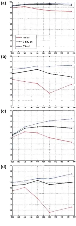
In this section, we will compare the effects of variations in domain sizes and strength of spectral driving on the total simulated fields. The spatial correlation coefficient between LBs and BB reference for each experiment are shown in the Figure 3 for the stationary component (left side column) and for the transient-eddy part (right side column). The spatial correlation coefficients show a systematic increase with SN strength, which is noteworthy given that only the large-scale part of the winds are affected directly by SN. There is no systematic variation of spatial correlation with domain sizes.
Panels a show the spatial correlation of the stationary and transient-eddy components for the 925hPa temperature field for various LB with BB simulations. For the stationary component, the correlation values are over 99% for ail experiments. For the transient-eddy component, the spatial correlations decrease notably with increasing domain size for the experiments without SN. Even with weak SN (0-5%), the correlations increase notably for ail domain sizes and improve further with increasing SN strength (SN 5%).
For the 700hPa rh field, the stationary component (Figure 3b) shows the correlation coefficients decreasing from 92.5% to 84% with the increase of domain size for the NO SN
18
experiment. For the transient-eddy component, a decrease of correlation with increasing domain size is also noted, although the decrease is not monotonic, possibly due to the insufficient sam pie size. Experiments with SN show higher correlation coefficients for both stationary and transient-eddy components, with the highest correlations being obtained for the stronger SN experiment with the largest domains.
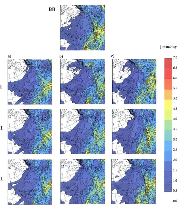
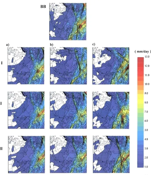
Precipitation is a very important quantity for the study of regional climate, but also a very demand ing quantity to correctly simulate because it is the end-product of complex interactions between the dynamical and physical parts of the model (Denis et aL, 2002b; Antic et al., 2004). Much of the central and northern parts of Canada have fairJy low precipitation amounts in winter. In the coastaJ area, the cold continental air masses and warmer air masses from the Atlantic come in contact; there is a mixture of precipitation with rain over the Atlantic area and mostly snow over the land. For the NO SN experiment, LBs 160 and 196 (Fig. 4 and 5) show different distribution of precipitation in the northern part of the window, with a patch of precipitation over the Forbisher Bay and the southern part of Baffin Island. The NO SN large-domain results have lower correlation values then other LBs (Fig. 3c). Nudging improves correlation and the values are over 98% for the stationary part (Fig. 3c); for the transient-eddy component, the values are somewhat lower but weil above 90%.
Until now, we have analyzed fields that are directly influenced by the surface forcing. The relative vorticity at 500hPa is much less directly influenced by the surface heterogeneities and is more driven by the nonlinear dynamics of the free atmosphere (Denis et al., 2002b; Antic et al., 2005). Although it is much more relevant for presenting small scales of the flow, we will briefly note the sensitivity of its total field. For the NO SN experiment, LB120 shows relatively high value of the correlation (93%) for the stationary component (Fig. 3d), which decreases drastically for the larger domains (Iess than 70%). For the transient-eddy component, ail LBs 100 have rather similar correlation coefficient, in the range of 65-70%. Experiments with SN show an increase of the correlation to over 80%, while the NO SN experiment shows a large drop of the correlation value for the LB16ü (60%).
19 In part, the increased correlation for both stationary and transient IS a direct consequence of enforcing through spectral nudging, the driving large scales that contain most of the variance.
4.2
Small scales
ln this section we will examine the small-scale features of the fields. As previously noted in our experimentaJ setup, the small-scales correspond to the scales smaller than 1080km and which therefore have been previously removed using a DCT filter in preparing the driving fields for the LB simulations. These scales were regenerated internally in the LB simulations, thus constitute the potential «added value}} of the CRCM simulations. The spatial correlation coefficients between LBs and BB reference for each experiment are shown in the Figure 6 for the stationary component (left side column) and for the transient-eddy part (right side column). The spatial correlation coefficients are smaller than for the total fields, which should not be surprising given that small scales are not driven by the lateral boundary conditions. We note again that stronger SN results in increased spatial correlation coefficients, despite the fa ct that SN only affects the large-scale component of the f1ow.
For the stationary part of the small-scale features of the 925hPa temperature field (figure 6a), the spatial correlation coefficient for the experiment without SN has values that show a tendency of decreasing with increasing domain size. The experiments with SN show the monotonie increase in correlation values that remain weil over 95%. For the transient eddy component, there is a visible decrease in correlation for the experiment without SN from 87% (LB 100) to the 73.5% (LB 196), while the SN experiments show an increase of correlation with increasing domain size.
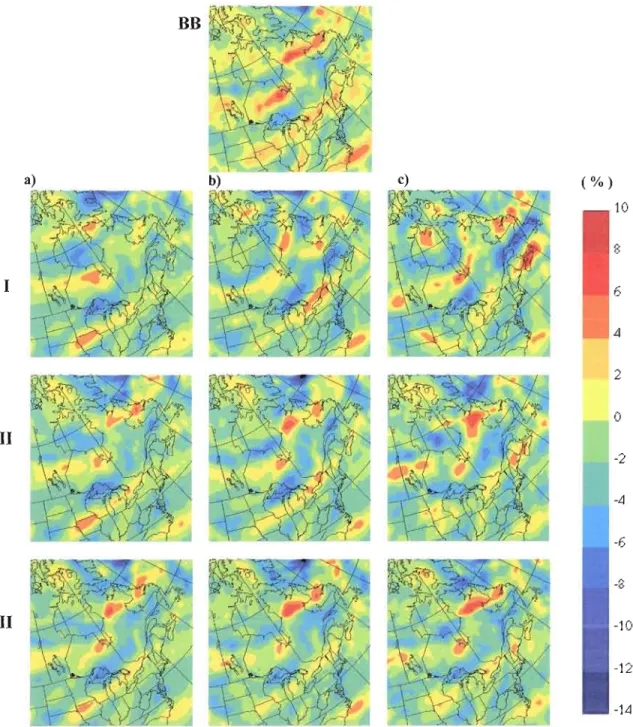
For the 700hPa rh field stationary component, the spatial correlation coefficient decreases significantly with increasing domain size for the NO SN experiment. The poorest correlation is noted for the LB 160 with a value of only 34% (Fig. 6b). With the application of SN we note an increase of correlation although the values are still around 80-83%. Ifwe look at the fields displayed on Figure 7, we see that the patterns show little resemblance with their reference. For the transient part ofthe 700hPa rh field, the correlations are much better. There
20
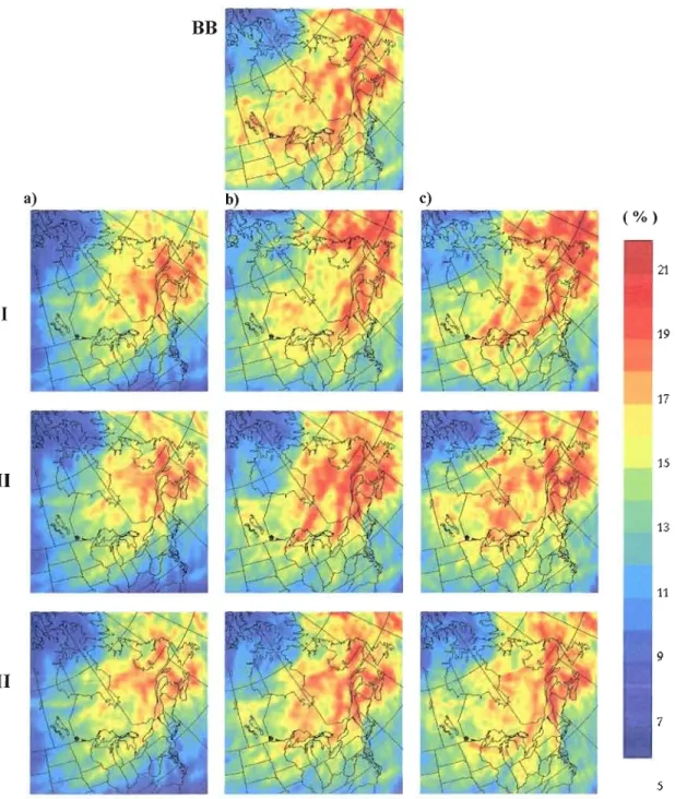
is a small but visible increase in the correlation values with increasing domain size in the NO SN experiment, and the increase is even more significant with SN; the values rise monotonically from 72.3% to 96.7% for the LB 160. The transient-eddy patterns also show high resemblance to their reference (Figure 8). For the smallest domain there is a significant presence ofthis underestimation in the inflow side of the domain which is in agreement to the results obtained by Leduc et al. (2008), and suggest the question of the spatial « spin-up » which extends from the inflow boundary.
If we now look at the stationary part of the precipitation field we can notice that there is a monotonic increase of correlation values with increased SN strength (Fig. 6c). The experiment without SN shows a decrease in correlation values with increasing domain sizes, from 62% (LB 120) to only 43% (LB 196). For the transient part of the field we can note behaviour similar to the relative humidity field, as the two are related. We can also note a spatial
«
spin-up» problem on the inflow side for the smaller domains, with a noticeable underestimation of the small-scale stationary (Fig. 9) and transient-eddy (Fig. 10) patterns in the inflow zone on the western side of the validation domain. CRCM precipitation is expected to be lower along the boundaries because vertical velocity is set to zero along the boundary; our validation domain excludes this zone however.The last field presented in this section is the 500hPa relative vorticity (rv) field. This field is useful to highlight the small-scale structure of the flow dynamics of the free atmosphere. It shows the poorest spatial correlation for its stationary part among the studied fields «17%). This might in part be a probJem reJated to the low time sampling, which interpret as stationary some eddies that are in fa ct transient; longer time averaging should produce improved correlations. SN in the experiments improves correlation for more than 50%, even with the weaker strength. Transient-eddy standard deviation of the SOOhPa rv field shows the exponential increase of the correlation values with increasing domain size for ail SN experiments, with the highest reached value close to 90%.
21
4.3
Taylor diagrams
The Taylor diagram is a way of plotting on a 2-D graph, using the law of cosine, three statistics that indicate how closely two model runs match each other. The three statistics are the relative mean square difference, the ratio of variances and the time correlation. The goal for the LB simulation is that it faIls as close as possible to the abscissa origin with a ratio of variance near 100%, a correlation of unity and vanishing mean square difference (Denis et al., 2002b). Taylor diagrams are here presented separately for large-scale (Figure II) and smaIl-scale (Figure 12) transient-eddy components of the following simulated field: pcp, temp, rh and rv. We will present the results for three LBs' domains (120, 160 and 196) and for the three SN strengths.
For the transient-eddy large-scale components (Fig. 11), we note a significant improvement in temporal correlation (R') with the increase of SN strength, as expected from the application of SN, and the correlation coefficients then become almost insensitive to domain size. Without SN, however, the correlation coefficients drop with increasing domain size, showing the weaker control exerted by the LBC. The large-scale variance ratios are close to unity for all domain sizes and for ail fields, except precipitation that is amplitude deficient on small domains due to spatial spin-up as discussed earlier.
Figure 12 presents the corresponding statistics for the transient-eddy small-scale component. For nearly all fields, we note sorne degree of underestimation of the transient eddy variance, which is more pronounced with smail domain sizes. The variance deficiency is most severe on small domain sizes, but the variance gradually asymptotes toward unity on the largest LB domain. This is particularly the case for precipitation that is more dominated by fine-scale features. We can also note a tendency for variance deficiency to increase with height, from the 700hPa rh field and even stronger for the 500hPa rv field; this is probably due to the fact that stronger winds at high altitudes require larger domain size for the complete development of the small-scale features. A domain size even larger than 196x196 grid points would be needed to test this hypothesis. The time correlation values are fairly modest and insensitive to domain size, but they tend to increase with SN strength, despite the
22
fact that SN does not directly affect the small scales; we speculate that small scales are somewhat preconditioned by large scales, which are improved by the application of SN.
23
5. Conclusion
The objective of this study is to examine the downscaling ability of a one-way nested CRCM by analyzing its sensitivity to domain size and large-scale driving technique. To address these issues, a perfect-model approach, nicknamed 'Big-Brother Experiment' was developed in a following way. A high-resolution large-domain simulation (Big Brother, BB) over a 250x250 grid-point domain is run for the months of January and February 1990. BB fields are used as a reference and filtered by removing small-scales in order to simulate the low-resolution present in the global models. The applied filter retained ail length scales longer than 2160km and removed those shorter than 1080km. Next, simulations were performed by the same model but over a small domain located inside the BB domain; these are called the Little Brothers (LB). Filtered BB fields provide the nesting data for the LB simulations. Different strengths of large-scale spectral nudging (SN) are applied to the large scales of horizontal wind; the main difference between the standard nesting approach and the SN is that large scales are not only imposed at the lateral boundaries but also forced within the regional domain. Finally, comparison of the LB with BB over a common zone informs us of the LB ability to regenerate the scales that were filtered and/or absent from the initial and lateral boundary conditions. Leduc et al. (2008) who studied the impact of different domain sizes on CRCM simulations used this approach. Here we have extended their study by further expanding domain sizes and applying SN.
Results have been presented for the time-average (stationary) and the transient-eddy components of the different fields and their small-scale features. The spatial correlation for total fields has shown little sensitivity to domain size, but a tendency for increase with stronger SN. For the smalJ-scale components, there is a decrease of spatial correlation with increasing domain size for the SN-free experiment; but for experiments with SN, we note an increase in correlation with increasing SN strength and domain size. The analysis has shown that this increase in correlation was present despite the fact that SN has been applied solely to the large-scale part of the horizontal wind components. Generally, LB patterns correlate better with BB for the smaller domains if no SN is applied; while with SN, LBs correlate better with BB for the larger domains.
24
In our results, we have noted sorne systematic underestimation in small-scale transient-eddy variance, particularly for precipitation as weil as for the relative humidity field near in the inflow zone of the domain. Knowing that these two fields are related lead us to assumption of the possible existence of the "spatial spin-up", which is defined as a characteristic distance from the lateral boundaries needed for a sufficient development of the small-scale features that are absent in the LBe. This spatial spin-up influence is also visible in the 500hPa rv field, which shows the poorest transient-eddy variance, possibly as a result of the insufficient development of the small scales due to the stronger winds in the troposphere and remoteness from surface forcing; t his field also shows the poorest correlation, which could be related to the low time sampling. Our study was based on one mon th statistics, which limits the strength for sorne of our conclusions; more definite conclusions could be obtained with longer time averaging in sorne forthcoming studies.
Our results have shown that the application of SN prevents regional model's solution to deviate from the driving fields and producing inconsistencies. The usage of perfect prognosis approach allowed us to visualize these differences by comparing runs that use the classic downscaling approach with SN driving runs. It also shows that SN technique leaves freedom to the CRCM to produce small-scale features. In summary, it allows us to use large domains to ensure the full development of small scales that are absent in the driving condition, while guarding the solution from going astray due to the development of intermittent divergence of solution in phase space (von Storch et al., 2000).
25
Acknowledgments
This research was done as a part of the Masters project within the Canadian Network for Regional Climate Modelling and Diagnostics (CRCMD), funded by the Canadian Foundation for Climate and Atmospheric Sciences (CFCAS). We wou Id also like to thank Mourad Labassi, Najet Labassi and Abderrahim KhaJed for maintaining a user-friendly local computing facility.
BIBLIOGRAPHIE
Alexandru A., R. de Elia., R. Laprise, L. Separovic and S. Biner, 2009: Sensitivity Study of
Regional Climate Model Simulation to Large-Scale Nudging Parameters. Monthly
Weather Review, Vol. 137, DOl 10.1 175/2008MWR2620. 1
Antic, S., R. Laprise, B. Denis, and R. de Elia, 2003: Testing the Downscaling Ability of a
One-Way Nested Regional Climate Model in regions of complex topography. C/im.
Dyn. 23,473-493.
Bechtold, P., E. Bazile, F. Guichard, P. Mascart, and E. Richard, 2001: A mass flux
convection scheme for regional and global models. Quarterly Journal of the Royal
Meteorological Society, 127. 869-886.
Biner, S., D. Caya, R. Laprise, and L. Spacek, 2000: Nesting of RCMs by imposing large
scales. Research Activities in Atmospheric and Oceanic Modelling, WMO/TD-987,
Rep. 30, H. Richie, Ed., WMO, 7.3-7.4.
Caya, D. and R. Laprise, 1999: A semi-implicit semi-Lagrangian regional climate model:
The Canadian RCM. Monthly Weather Review, 127,341-362.
Davies, H.
c.,
1976: A lateral boundary formulation for multi-level prediction models.QuarterlyJournal ofthe Royal Meteorological Society, 102: 405-418.
Denis, B., J. Côté, and R. Laprise, 2002a: Spectral decomposition of two-dimensional atrnospheric fields on limited-area domains using the discrete cosine transform (DCT).
Monthly Weather Review, 130, 1812-1829.
- ' R. Laprise, D. Caya, 1. and Côté, 2002b: Downscaling ability of a one-way nested
regional climate mode!: The Big-Brother Experiment. C/imate Dynamics, 18: 627-646.
Dickinson, R. E., R. M. Errico, F. Giorgi, and G. T. Bates, 1989: A regional climate model
for the Western United States. C/imate Change, 15,383-422.
Gal-Chen, T., and R. C. J. Somervilie, 1975: On the Use of a Coordinate Transformation for
the Solution of the Navier-Stokes Equations. Journal of Computational Physics, 17,
27
Giorgi, F., 1990: Simulation of regional climate L1sing a limited area model nested In ageneral circulation mode!. Journal ofClimate, 3, 941-963.
_ _, and L. O. Meams, 1999: Introduction to special section: Regional climate modelling revisited. Journal ofGeophysical Research, 104,6335-6352.
Jones R. G., 1. M. Murphy, and M.Noguer, 1995: Simulation of climate change over Europe using a nested regional-climate model. I:assessment of control climate, including sensitivity to location of lateral boundaries. . Quarterly Journal of the Royal Meteorological Society,121: 1413-1449
Kain, J. S. M. and 1. M. Fritsch, 1990: A one-dimensional entrainingldetraining plume model and its implication in convective parameterization. Journal of the Atmospheric Sciences, 47,2784-2802.
Laprise, R. D. Caya, M. Giguère, G. Bergeron, H. Côté, J.-P. Blanchet, G. J. Boer, and N. A. McFariane, 1998: Climate and c1imate change in western Canada as simulated by the Canadian Regional Climate Model. Atmosphere-Ocean, 36, 119-167.
_ _, 2008: Regional climate modelling. Journal of Computational Physics, Special issue on 'Predicting weather, climate and extreme events', 227,3641-3666.
Leduc, M., and R. Laprise, 2008: Regional climate model sensitivity to domain size. Climate Dynamics, 32, 833-854, doi: 10.1007/s00382-008-0400-z.
Miguez-Macho, G., G. L. Stenchikov, and A. Robock, 2004: Spectral nudging to eliminate the effects of domain position and geometry in regional climate model simulations. Journal ofGeophysical Research, 109, D13104, doi: 10.1 029/2003JD004495.
Plummer, D. A., D. Caya, H. Côté, A. Frigon, S. Biner, M. Giguère, D. Paquin, R. Harvey, de Elia, 2006: Climate and climate change over North America as simulated by the Canadian RCM. Journal ofClimate, 19,3112-3132.
Robert, A., and E. Yakimiw, 1986: Identification and elimination of an inflow boundary computational solution in limited area model integrations. Atmosphere-Ocean, 24, 369 385.
Taylor, K. E., 2001: Summarizing multiple aspects of mode! performance In a single
28
von Storch, H., H. Langenberg, and F. Feser, 2000: A spectral nudging technique for
dynamical downscaling purposes. Monthly Weather Review, 124, 529-547.
_ _, H., E. Zorita and U. Cubasch, 1993: Downscaling of global climate change estimates
to regional scales: An application to Iberian rainfall in wintertime. 1. Climate 6, J 161
1171.
Waldron, K. M., J. Peagle, and J. D. Horel, 1996: Sensitivity of a spectrally filtered and
nudged limited area model to outer model options. Monthly Weather Review, 124, 529
547.
Yakimiw, E., and Robert, 1990: Validation experiments for a nested grid-point regional
30
Figure 1 Schematics of the Big-Brother (BB) experimental protocol a The BB high-resolution simulation with the area of interest (dashed line) b The BB solution after using the low-pass filter c The Little-Brother (LB) high-resolution simulation.
31
Figure 2 The computational domains of the Big Brother (BB: 196xJ96 grid points) and the Little
Brothers (LBI to LBS) having respectively 196x196, J60xJ60, J40x140, 120xl2ü and IOOxlOO grid points. The climate statistics are verified through the QC area (dashed) of 86x86 grid points.
32
(a) (b) (c) (d) ,0<)'"
Il(l ...~. '" ro,.
70 60 60 so so '" '" JO ".,
...• '" '7", '00Il.
'20 ,JO".
'so 160".
,ro '00 200 '1", 110".
,JO'''' ISO W, '00
,.,
200 • • d • •'"
00,.
,....
'"'"
so..
'" '" " .,.,
... ; '100,..,
Il.
".
'"
,
..
100"'"
,.., '100Il.
".
'''',.,
'so '''' ,,. '00 '00 200 . . ;-..
"'~'"
,.
,.
'" '" so so..
'" '" .. "'"
.
'100 110 '00
...
'so 160 '00 'SO 200 '100Il.
,JO 'SO '70 '00 '00""
".
'''' '''' ''''""
'00 "".
... Il(l 00..
'" 50 so..
'" "'. " '" '" 'l",Il.
,'"
,..
.00 ,,. '00 200 '?oo 0" ,,. '''' """"
'''' '''' ''''Figure 3 Spatial correlation of LB with BB for the stationary (Jeft side column) and transient-eddy standard deviation (right side column), as a function of LB domain size and SN strength: a 925hPa temperature b 700hPa relative humidity c precipitation d 500hPa relative vorticity.
33
BB
(mm/day) c) 7.0 65 6.0 1 55 5.0 45 4.0 II 3.5 3.0 25 2.0 15 III 1.0 0.5 0.0Figure 4 Stationary component of the precipitation rate field for the LBs a 120 b 160 and c 196 for the different experiments with 1 no SN II 0-5% SN and III 5% SN.
34
BB b) (mm/day) 13.0 1 12.0 11.0 10.0 9.0II
80 Î.O 6.0 5.0 4.0III
3.0 2.0 1.0 0.0Figure 5 Transient componeot of the precipitation rate field for the LBs a 120 b 160 and c 196 for the
35 (a) (b) (c) (d) "" 100 ·i··· 00 00 70 60 60 60 60
..
'" ... no sn » ---+-0-5% sn ··-5%sn '" 10 100 110 '''' 13" "" 1,. '''' 170 100 100 200 '100 110''''
1» l''' 150 160 170 '00 100 200 100 100 90· 90 ... 00 70 111 ...--.. ... ~.. 60 00 50 '" '"..
... ~ '" " '100 120 l''' 150 '60 170 100 100 200 '100 '10 120 150 160 '70 100 100 200 '" """"
"" 100 '00 00 00 oo~ 60 ..,... 60 '" ~.-.; ." >J >J 20 10 • '00 110 120 1» 150 '70 100 '00 200 '100 '10 120 1>J '60 100 100 100 200 '''' "" '00 100 00 00 00 '" 60'"
...,.. '" <O . ." >J '" 20 '" '100 110 1» ,." 160 '00 "" '00 '00 "" '''' '100 110 '50 '''' 170 100 '00 200""
""Figure 6 Spatial correlation of LB with BB for the small-scale stationary (left side column) and transient-eddy standard deviation (right side column), as a function of LB domain size and SN strength: a 925hPa temperature b 700hPa relative humidity c precipitation d 500hPa relative vorticity.
36
BB
a) (% ) 10 8 1 6 4 L '"' 0II
-2 -4 -6 (-. -6III
-10 -12 -14Figure 7 Small-scale stationary component of the 700hPa relative humidity field for the LBs a 120 b 160 and c 196 for the different experiments with 1 no SN Il 0-5% SN and III 5% SN.
37
BB
(% ) 1 :<1 19 17 II 1.5 13 11III
9 7 .5Figure 8 Small-scale transient component of the 700hPa relative humidity field for the LBs a 120 b 160 and c 196 for the different experiments with 1 no SN Il 0-5% SN and III 5% SN
38
BB
Figure 9 Small-scale stationary component of the precipitation field for the LBs a 120 b 160 and c 196 for the different experiments with 1 no SN Il 0-5% SN and III 5% SN.
39
BB
(mm/day) 10.0 1 9.0 8.0 7.0II
6.0 5.0 4.0 3.0 III 0.0 figure 10 Small-scaJe tTansient component of the precipitation field for the LBs a 120 b J60 and c 196 for the different experiments with 1 no SN 11 0-5% SN and [II 5% SN.40
a) b) 1')0 5D 100 00 0' .... .c ~ " 50~ 50 .~"
01-""
/o~ 25~ la o 1 5 la 75 50 100 (rmsd/sig"" )' c) d) 151 100 f .' 50·~"
la a , 5 la 25 50 100 la o 1 5 10 25 50 100 (rmSd/sig.. )' (rmSd/S'g., )' 120 NO SN 160 NO SN • 196 NO SN .. 120 SN 0-5% .. 160 SN 0-5% .. 196 SN 0-5% • 120SN5% • 160 SN 5% • 1965N5%Figure Il Taylor diagrams for the transient-eddy large-scale component of a precipitation rate, b
925hPa temperature, c 700hPa relative humidity and d SOOhPa relative vorticity fields, for different experiments.
41
a) b) 100 100 Jl - 50t
50 -~ ... ... o o 1 ~ la 25 :'0 100 10 o 1 5 10 25 50 100 (rmsd/sigo • )~ (r'l'1sd/sig.., )~ c) d) N...
-il ~ 50 ïii'"
50 ïii'"
... ... -" -" 0' 0' ?5~ 25~ 10 0 1 5 la 25 50 100 (rmsd/sig", )'•
120 NO SN•
160 NO SN•
196NOSN•
120 SN 0-5%•
160 SN 0-5%•
196 SN 0-5%•
120 SN 5%•
160 SN 5%•
1965N5%Figure 12 Taylor diagrams for the transient-eddy small-scale component of a precipitation rate, b 925hPa temperature, c 700hPa relative humidity and d 500hPa relative vorticity fields, for different experiments.