Solute transport modelling at the groundwater body scale: Nitrate trends assessment in the Geer basin (Belgium)

Texte intégral

(1)Université de Liège Faculté des Sciences Appliquées Département ArGEnCo Architecture, Géologie, Environnement et constructions. Secteur GEO³ Géotechnologies, Hydrogéologie, Prospection Géophysique. Solute transport modelling at the groundwater body scale: Nitrate trends assessment in the Geer basin (Belgium) Thèse de doctorat présentée par Philippe ORBAN en vue de l’obtention du grade de Docteur en Sciences de l’Ingénieur. Soutenue devant le jury composé de : R. CHARLIER, Université de Liège (Belgique) – Président A. DASSARGUES, Université de Liège (Belgique) – Promoteur S. BROUYERE, Université de Liège – Co-promoteur E. DELHEZ, Université de Liège (Belgique) M. PIROTTON, Université de Liège (Belgique) V. HALLET, Facultés Universitaires Notre-Dame de la Paix, Namur (Belgique) R. THERRIEN, Université Laval (Canada) J.-M. LEMIEUX Eidgenössische Technische Hochschule Zürich (Suisse) J. BARTH, GeoZentrum Nordbayern, Erlangen-Nürnberg (Allemagne). Novembre 2008.

(2)

(3) Abstract. ABSTRACT Water resources management is now recognized as a multidisciplinary task that has to be performed in an integrated way, within the natural boundaries of the hydrological basin or of the aquifers. Policy makers and water managers express a need to have tools able at this regional scale to help in the management of the water resources. Until now, few methodologies and tools were available to assess and model the fate of diffuse contaminants in groundwater at the regional scale. In this context, the objective of this research was to develop a pragmatic tool to assess and to model groundwater flow and solute transport at the regional scale. A general methodology including the acquisition and the management of data and a new flexible numerical approach was developed. This numerical approach called Hybrid Finite Element Mixing Cell (HFEMC) was implemented in the SUFT3D simulator developed by the Hydrogeology Group of the University of Liège. A first application of this methodology was performed on the Geer basin. The chalk aquifer of the Geer basin is an important resource of groundwater for the city of Liège and its suburbs. The quality of this groundwater resource is threatened by diffuse nitrate contamination mostly resulting from agricultural practices. New field investigations were performed in the basin to better understand the spatial distribution of the nitrate contamination. Samples were taken for environmental tracers (tritium, CFC’s and SF6) analysis. The spatial distribution of environmental tracers concentrations is in concordance with the spatial distribution of nitrates. This allows proposing a coherent interpretative schema of the groundwater flow and solute transport at the regional scale. These new data and the results of a statistical nitrate trend analysis were used to calibrate the groundwater model developed with the HFEMC approach. This groundwater flow and solute transport model was used to forecast the evolution of nitrate concentrations in groundwater under a realistic scenario of nitrate input for the period 2008-2058. According to the modelling results, upward nitrate trends observed in the basin will not be reversed for 2015 as prescribed by the EU Water Framework Directive.. 1.

(4) Abstract The regional scale groundwater solute transport model was subsequently used to compute nitrate concentrations in groundwater under different scenarios of nitrate input to feed a socioeconomic analysis performed by BRGM. These computed concentrations were used to assess the benefit, for the users, linked to the reduction of contamination resulting from the changes in nitrate input. These benefits were compared to the costs associated to the implementation of the considered agri-environmental schemes that allow reducing the nitrate input to groundwater.. 2.

(5) Résumé. RESUME La gestion des ressources en eaux souterraines est actuellement reconnue comme une tâche multidisciplinaire devant être réalisée, de manière intégrée, au sein des frontières naturelles des bassins hydrologiques ou des aquifères. Les politiciens et gestionnaires des ressources en eaux requièrent des outils capables, à cette échelle, d’aide à la gestion des ressources en eaux. A ce jour, peu de méthodologies et d’outils sont disponibles pour évaluer et modéliser le devenir de pollutions diffuses dans les eaux souterraines à l’échelle régionale. Dans ce contexte, l’objectif de cette recherche est de développer un outil pragmatique pour évaluer et modéliser les écoulements et le transport de solutés dans les eaux souterraines à l’échelle régionale. Une approche générale a été développée qui inclut l’acquisition, le traitement de données et une nouvelle approche numérique flexible. Cette approche, appelée « Hybrid Finite Element Mixing Cell » (HFEMC), a été implémentée dans le code SUFT3D développé par le Groupe d’Hydrogéologie de l’Université de Liège. Une première application de cette méthodologie a été réalisée pour le bassin du Geer (480 Km2). L’aquifère crayeux de ce bassin est une ressource importante en eaux souterraines pour la ville de Liège et ses faubourgs. La qualité de cette eau souterraine est menacée par une contamination diffuse en nitrate résultant principalement des pratiques agricoles. De nouvelles investigations de terrain ont été réalisées dans le bassin afin de mieux comprendre la distribution spatiale de la pollution en nitrate. Des échantillons ont été prélevés pour analyse des concentrations en traceurs environnementaux (tritium, CFCs et SF6). La distribution spatiale des concentrations en traceurs environnementaux est en concordance avec la distribution spatiale des nitrates. Cela permet de proposer un schéma cohérent d’interprétation des écoulements d’eaux souterraines et de transport de solutés à l’échelle de l’aquifère. Ces nouvelles données ainsi que les résultats d’une étude statistique des tendances des nitrates ont été utilisés pour calibrer le modèle eau souterraine développé à l’aide de l’approche HFEMC. Ce modèle d’écoulement des eaux souterraines et de transport de soluté a été employé pour prédire l’évolution, pour la période 2008-2058, des concentrations en nitrate dans les eaux souterraines pour un scénario réaliste d’apport de nitrate. Au regard des résultats de modélisation, les tendances à la hausse observées dans le bassin ne seront pas. 3.

(6) Résumé inversées pour 2015 comme requis par la Directive Cadre sur l’Eau de la Commission Européenne. Le modèle de transport de soluté dans les eaux souterraines à l’échelle régionale a été utilisé pour calculer les concentrations en nitrate dans les eaux souterraines pour différents scénarios d’apport en nitrate afin d’alimenter une analyse socio-économique réalisée par le BRGM. Ces concentrations calculées ont été utilisées afin d’évaluer les bénéfices, pour les utilisateurs, liés à la réduction de la contamination résultant des changements dans l’input nitrate. Ces bénéfices ont été comparés aux coûts associés à l’implémentation des mesures agroenvironnementales qui permettent de réduire l’input nitrate vers les eaux souterraines... 4.

(7) Acknowledgments. ACKNOWLEDGMENTS At the end of my Master study, when Professor Dassargues asked me to work in his team first as a PhD student and later as an assistant, I never thought to finalise a PhD thesis. During seven years, I have been confronted to various tasks, sometimes very different of my PhD thesis works. Nevertheless, this manuscript is the proof that this research has succeeded. This study is integrated with the works developed by the Hydrogeology Group of the University of Liège for years now as well in the domain of regional scale modelling as in the domain of the study of the hydrogeology of the Geer basin. This thesis was supervised by Alain Dassargues and Serge Brouyère. First of all, I would like to thank them for supporting me and for their guidance during these years. I’m also grateful for the anticipating reading of the work they have done, as well as for proposals and suggestions to improve its quality. I would also thank Alain Dassargues for giving me the opportunity to work with him as an assistant. He always trusted me during these years both for pedagogical tasks and for research works. It is a chance and a pleasure to work with Serge Brouyère. Thank you Serge, you introduced me to research and encouraged me to go further in my works. I would like to thank Robert Charlier, Michel Pirotton, Eric Delhez, Vincent Hallet, René Therrien, Jean-Michel Lemieux and Johannnes Barth who accepted to devote a piece of their time to read this manuscript and to be members of this jury. The Hydrogeology Group is really a pleasant working environment thanks to the people there. Thanks to all my colleagues Jordi, Ingrid, Horatiu, Marie, Cristina, Nicolas, Julie G., Laurent P., Laurent T., Julie C., Angaman, Gaëlle, Tanguy, Jean, David, Pierre ad Fred for all these good times, for their help and their interesting hydrogeological or non-hydrogeological discussions. I would like particularly to thank Jordi and Ingrid. Thank you Ingrid for supporting me during all these years and for your sound advices as well concerning database or mapping techniques. And thank you Jordi for all these good times we have shared in our office, along the Mediterranean Sea or in a yellow caravan. This last year of work has been, for some aspect, difficult but you have always been there for an advice or talk.. 5.

(8) Acknowledgments Thank to Bernard Belot for the chemical analysis of major ions and to Professor Malozewski and his team for the tritium analysis. Thanks are also due to Annick Anceau and the team of the Earth Science library for helping me in my research of unobtainable papers. A particular thanks to Cécile Hérivaux from the BRGM team for our fruitful collaboration regarding the socio-economic study performed on the Geer basin in the framework of the AquaTerra project. Many thanks to Martine, Nadia and Christiane the secretary staff who are always present and available. When developing model at the regional scale, lots of data have to be collected. I would like to thank the team of the CILE, SWDE and VMW companies and the team of the DGRNE for their warm welcomes, the data they have provided and their enthusiasm regarding my work. Thanks to the University of Liège for giving me the opportunity through its funding to performed this work. Many thanks to the Administration of the Walloon Region for funding parts of this work through the PIRENE project or the environmental tracer surveys. Conceptual and numerical developments of the HFEMC method have also been performed in the framework of the Interuniversity Attraction Pole TIMOTHY (IAP Research Project P6/13) funded by the Belgian Federal Science Policy Office (BELSPO) and the European Integrated Project AquaTerra (GOCE 505428) funded by the Community’s Sixth Framework Programme.. Finally, I am very grateful to all my family for continuously supporting all along my studies. During these seven years, I have had the happiness to marry you Delphine and then to welcome Chloé and Nathan who have extended our family. Thanks to you for your help and your patience.. 6.

(9) Knowledge dissemination. KNOWLEDGE DISSEMINATION List of publications •. Barth, J. A. C., P. Grathwohl, H. J. Fowler, A. Bellin, M. H. Gerzabek, G. J. Lair, D. Barcelo, M. Petrovic, A. Navarro, P. Négrel, E. Petelet-Giraud, D. Darmendrail, H. Rijnaarts, A. Langenhoff, J. de Weert, A. Slob, B. M. van der Zaan, J. Gerritse, E. Frank, A. Gutierrez, R. Kretzschmar, T. Gocht, D. Steidle, F. Garrido, K. C. Jones, S. Meijer, C. Moeckel, A. Marsman, G. Klaver, T. Vogel, C. Bürger, O. Kolditz, H. P. Broers, N. Baran, J. Joziasse, W. Von Tümpling, P. Van Gaans, C. Merly, A. Chapman, S. Brouyère, J. Batlle Aguilar, Ph. Orban, N. Tas and H. Smidt (2008). "Mobility, turnover and storage of pollutants in soils, sediments and waters: achievements and results of the EU project AquaTerra. A review." Agronomy for sustainable development 28. DOI: 10.1051/agro.2007060.. •. Barth, J. A. C., E. Kalbus, C. Schmidt, M. Bayer-Raich, F. Reinstorf, M. Schirmer, D. Thiéry, I. G. Dubus, A. Gutierrez, N. Baran, C. Mouvet, E. Petelet-Giraud, P. Négrel, O. Banton, J. Batlle Aguilar, S. Brouyère, P. Goderniaux, Ph. Orban, J. C. Rozemeijer, A. Visser, M. F. P. Bierkens, B. Van der Grift, H. P. Broers, A. Marsman, G. Klaver, J. Slobodnik and P. Grathwohl (2007). "Selected groundwater studies of EU project AquaTerra leading to large-scale basin considerations." Water Practice & Technology 2(3). DOI: 10.2166/WPT.2007062.. •. Batlle-Aguilar, J., Ph. Orban, A. Dassargues and S. Brouyère (2007). "Identification of groundwater quality trends in a chalk aquifer threatened by intensive agriculture in Belgium." Hydrogeology Journal 15: 1615-1627.. •. Brouyère, S., Ph. Orban, S. Wildemeersch, J. Couturier, N. Gardin and A. Dassargues. "The hybrid finite element mixing cell method: a new flexible method for modelling mine water problems." Mine Water and the Environment: In press.. •. Hérivaux, C., Ph. Orban, J. Batlle-Aguilar, P. Goderniaux and S. Brouyère. "Socioeconomic analysis integrating soil-water system modelling for the Geer catchment (Meuse, Walloon region) - diffuse nitrate pollution in groundwater." Manuscript in preparation.. •. Orban, Ph., S. Brouyère, J. Couturier, P. Goderniaux, J. Batlle-Aguilar and A. Dassargues. "Modelling nitrate trends in groundwater at the regional scale using the HFEMC approach: Application to the chalk aquifer of the Geer basin (Belgium)." Manuscript in preparation for submission to the Journal of Contaminant Hydrology.. •. Orban, Ph., C. Popescu, I. Ruthy and S. Brouyère (2004). "Database and general modelling concepts for groundwater modelling in the Squash project." Hidrotehnica 49(9-10): 51-57.. •. Visser, A., M. F. P. Bierkens, I. G. Dubus, J.-L. Pinault, N. Surdyk, D. Guyonnet, J. Batlle-Aguilar, S. Brouyère, P. Goderniaux, Ph. Orban, M. Korcz, J. Bronder, J. Dlugosz and M. Odrzywolek. "Comparison of methods for the detection and extrapolation of trends in groundwater quality." Manuscript in preparation.. 7.

(10) Knowledge dissemination. Conference proceedings •. Batlle-Aguilar, J., Ph. Orban, A. Dassargues and S. Brouyère (2006). Identification of groundwater quality trends in a chalky aquifer threatened by intensive agriculture. International Association for Mathematical Geology, XIth Congress, Liège (Belgium).. •. Batlle-Aguilar, J., Ph. Orban, A. Dassargues and S. Brouyère (2007). Identification of groundwater quality trends in a chalky aquifer threatened by intensive agriculture. Diffuse inputs into the groundwater: Monitoring - Modelling - Management, Graz (Austria).. •. Brouyère, S., Ph. Orban, S. Wildemeersch, J. Couturier, N. Gardin and A. Dassargues (2008). The Hybrid Finite Element Mixing Cell method: a new flexible method for modelling mine water problems. Mine Water and the Environment: 10th International MineWater Association Congress, Karlovy Vary (Czech Republic).. •. Orban, Ph., J. Batlle-Aguilar, A. Dassargues and S. Brouyère (2006). Large-scale groundwater flow and transport modeling: Methodology and application to the Geer basin, Belgium. International Association for Mathematical Geology, XIth Congress, Liège (Belgium).. •. Orban, Ph., S. Brouyère, H. Corbeanu and A. Dassargues (2005). Large-scale groundwater flow and transport modelling: methodology and application to the Meuse Basin, Belgium. Bringing Groundwater Quality Research to the Watershed Scale, 4th International Groundwater Quality conference, IAHS, Waterloo, Canada.. Scientific report PIRENE project •. Brouyère, S., H. Corbeanu, M. Dachy, N. Gardin, Ph. Orban and A. Dassargues (2004). Projet de recherche PIRENE: Rapport final, DGRNE: 105.. •. Brouyère, S., Ph. Orban, H. Corbeanu and A. Dassargues (2003). Projet de recherche PIRENE: 3ème Rapport annuel DGRNE: 77.. •. Brouyère, S., Ph. Orban, A. Dassargues and A. Monjoie (2001). Projet de recherche PIRENE: 1er Rapport annuel DGRNE: 43.. •. Brouyère, S., Ph. Orban, A. Dassargues and A. Monjoie (2002). Projet de recherche PIRENE: 2ème Rapport annuel, DGRNE: 50.. 8.

(11) Knowledge dissemination AquaTerra project •. Broers, H. P., A. Visser, M. F. P. Bierkens, I. G. Dubus, J.-L. Pinault, N. Surdyk, D. Guyonnet, J. Batlle-Aguilar, S. Brouyère, P. Goderniaux, Ph. Orban, M. Korcz, J. Bronder, J. Dlugosz and M. Odrzywolek (2008). Draft overview paper on trend analysis in groundwater summarizing the main results of TREND2 in relation to the new Groundwater Directive. Deliverable T2.12, AquaTerra (Integrated Project FP6 no. 505428): 46.. •. Broers, H. P., A. Visser, I. G. Dubus, N. Baran, X. Morvan, M. Normand, A. Gutiérrez, C. Mouvet, J. Batlle Aguilar, S. Brouyère, Ph. Orban, S. Dautrebande, C. Sohier, M. Korcz, J. Bronder, J. Dlugosz and M. Odrzywolek (2005). Report with documentation of reconstructed land use around test sites. Deliverable T2.2, AquaTerra (Integrated Project FP6 no. 505428): 64.. •. Broers, H. P., A. Visser, R. Heerdink, B. Van der Grift, N. Surdyk, I. G. Dubus, N. Amaoui, Ph. Orban, J. Batlle-Aguilar, P. Goderniaux and S. Brouyère (2008). Report which describes the physically determinstic determination and extrapolation of time trends at selected test locations in Dutch part of the Meuse Basin, the Brévilles catchment and the Geer catchment. Deliverable T2.10, AquaTerra (Integrated Project FP6 no. 505428): 47.. •. Broers, H. P., A. Visser, R. Heerdink, B. Van der Grift, N. Surdyk, I. G. Dubus, A. Gutierrez, Ph. Orban and S. Brouyère (2007). Report with results of groundwater flow and reactive transport modelling at selected test locations in Dutch part of the Meuse basin, the Brévilles catchment and the Geer catchment. Deliverable T2.8, AquaTerra (Integrated Project FP6 no. 505428): 26.. •. Broers, H. P., A. Visser, R. Heerdink, B. Van der Grift, N. Surdyk, I. G. Dubus, A. Gutierrez, Ph. Orban and S. Brouyère (2007). Short report describing the progress of the groundwater flow and reactive transport modelling and elucidating interactions with COMPUTE and HYDRO and FLUX workpackages. Deliverable T2.7, AquaTerra (Integrated Project FP6 no. 505428): 35.. •. Broers, H. P., A. Visser, J.-L. Pinault, D. Guyonnet, I. G. Dubus, N. Baran, A. Gutierrez, C. Mouvet, J. Batlle-Aguilar, Ph. Orban and S. Brouyère (2005). Report on extrapolated time trends at test sites, Deliverable T2.4, AquaTerra (Integrated Project FP6 no. 505428): 81.. •. Broers, H. P., A. Visser, B. Van der Grift, I. G. Dubus, Guttierrez, C. Mouvet, N. Baran, Ph. Orban, J. Batlle-Aguilar and S. Brouyère (2006). Input data sets and short report describing the subsoil input data for groundwater and reactive transport modelling at test locations in Dutch part of the Meuse basin, the Brévilles catchment and the Geer catchment. Deliverable T2.5, AquaTerra (Integrated Project FP6 no. 505428): 23.. •. Dubus, I. G., J.-L. Pinault, N. Surdyk, D. Guyonnet, H. P. Broers, A. Visser, Ph. Orban, J. Batlle-Aguilar, P. Goderniaux and S. Brouyère (2008). Report with comparison of statistical and physically deterministic methods of trend assessment and. 9.

(12) Knowledge dissemination extrapolation in terms of data requirements, costs and accuracy. Deliverable T2.11, AquaTerra (Integrated Project FP6 no. 505428): 33. •. Hérivaux, C., Ph. Orban, J. Batlle-Aguilar, S. Brouyère and P. Goderniaux (2008). Socio-economic analysis integrating soil-water system modelling for the Geer catchment (Meuse, Walloon region) - diffuse nitrate pollution in groundwater. Deliverable I3.8, AquaTerra (Integrated Project FP6 no. 505428): 45.. •. Orban, Ph., J. Batlle-Aguilar, P. Goderniaux, A. Dassargues and S. Brouyère (2006). Description of hydrogeological conditions in the Geer sub-catchment and synthesis of available data for groundwater modelling. Deliverable R3.16, AquaTerra (Integrated Project FP6 no 505428): 20.. •. Orban, Ph. and S. Brouyère (2006). Groundwater flow and transport delivered for groundwater quality trend forecasting by TREND T2. Deliverable R3.18, AquaTerra (Integrated Project FP6 no 505428): 20.. Synclin’Eau Project •. Lorenzini, G., Ph. Orban, S. Brouyère and A. Dassargues (2008). Note méthodologique relative à la modélisation hydrogéologiques des masses d'eau souterraine RWM011, RWM012 et RWM021 (aspects quantitatifs et qualitatifs) Synclin'Eau. Convention RW et SPGE - Aquapôle: 26.. 10.

(13) Table of contents. TABLE OF CONTENTS Acknowledgments…………………………………………………………………………….. 5 Knowledge dissemination……………………………………………………………………...7 List of the main symbols……………………………………………………………………...15 List of the main acronyms………………………………………………………………….…17 1. INTRODUCTION.......................................................................................................... 19 1.1 1.2 1.3. 2. Context of the research............................................................................................. 21 The PIRENE and AquaTerra projects...................................................................... 22 Objectives of the research ........................................................................................ 23. REVIEW OF THE LITERATURE.............................................................................. 25 2.1 2.2. Representative Elementary Volume......................................................................... 27 Migration of solutes in groundwater ........................................................................ 27. 2.2.1 2.2.2 2.2.3 2.2.4 2.2.5. 2.3. Advection .................................................................................................................... 28 Hydrodynamic dispersion ........................................................................................... 31 Degradation ................................................................................................................. 33 Retardation and trapping ............................................................................................. 33 Solute transport equations ........................................................................................... 36. Existing approaches for modelling solute transport in groundwater at the regional scale………………………………………………………………………………...36. 2.3.1 2.3.1.1 2.3.1.2 2.3.2 2.3.3 2.3.3.1 2.3.3.2 2.3.4. 2.4 2.5 2.6 2.7 3. Transfer function models ............................................................................................ 36 Non-parametric transfer functions ......................................................................... 38 Transfer functions based on empirical or physical mathematical models.............. 38 Compartment models .................................................................................................. 43 Advection-dispersion models applied at the regional scale ........................................ 44 Parametrisation ...................................................................................................... 45 Numerical solution to the advection-dispersion equation ...................................... 46 Comparisons between the approaches of the transfer function type and the spatiallydistributed models ....................................................................................................... 48. Nitrates in groundwater............................................................................................ 50 Environmental tracers .............................................................................................. 52 Quality trend assessment in groundwater................................................................. 55 References to chapter 2 ............................................................................................ 58. THE HYBRID FINITE ELEMENT MIXING CELL APPROACH ........................ 69 3.1 3.2 3.3. The need for regional scale groundwater model ...................................................... 71 Specificities of regional scale groundwater modelling ............................................ 71 General methodology ............................................................................................... 73. 3.3.1 Data management and processing ............................................................................... 73 3.3.2 The Hybrid Finite Element Mixing Cell approach...................................................... 74 3.3.2.1 Concepts.................................................................................................................. 74 3.3.2.2 Adapted version of the SUFT3D code: Hybrid Finite Element Mixing Cell (HFEMC) method ................................................................................................... 78 3.3.3 Development of interfaces .......................................................................................... 84 3.3.3.1 Cutting the mesh into subdomains .......................................................................... 84 3.3.3.2 Definition of river boundary conditions.................................................................. 86. 11.

(14) Table of contents 3.3.3.3. 3.4. Creation of the input files for the SUFT3D............................................................. 87. Test of the HFEMC approach implemented in the SUFT3D code .......................... 88. 3.4.1 Validation of the flow equations implemented in the SUFT3D.................................. 88 3.4.1.1 Comparison of the linear reservoir solution and an analytical solution ................ 88 3.4.1.2 Comparison with an analytical solution for combination of a linear reservoir and a traditional approach in a column ........................................................................... 90 3.4.1.3 Comparison with an analytical solution for combination of a linear reservoir and a traditional approach in a 3D model ....................................................................... 91 3.4.2 Validation of the implementation of the transport equations in the SUFT3D............. 93 3.4.2.1 Comparison of the mixing cell solution of the SUFT3D and a semi-analytical solution 93 3.4.2.2 Transport from a point source in a uniform two-dimensional flow field ................ 96 3.4.2.3 Comparison of mixing cell and advection dispersion solutions in a saturated column 98 3.4.2.4 Comparison of mixing cell and advection dispersion solutions in a 2D problem ……………………………………………………………………………. 100 3.4.2.5 Example MIM from van Genuchten (1976) .......................................................... 101 3.4.3 Conclusions of the tests............................................................................................. 103. 3.5 4. References to chapter 3 .......................................................................................... 104. CASE STUDY: THE GEER BASIN .......................................................................... 107 4.1 4.2. Introduction ............................................................................................................ 109 Description of the Geer basin................................................................................. 110. 4.2.1 Geographical and geomorphologic context............................................................... 110 4.2.2 Geological context..................................................................................................... 111 4.2.3 Hydrogeological context ........................................................................................... 113 4.2.3.1 Data on groundwater abstraction......................................................................... 113 4.2.3.2 Piezometry ............................................................................................................ 114 4.2.3.3 Time evolution of the piezometry .......................................................................... 115 4.2.3.4 Limit of the hydrogeological basin ....................................................................... 117 4.2.3.5 Hydrogeological water budget ............................................................................. 118 4.2.3.6 Hydrodynamics of the chalk aquifer ..................................................................... 119 4.2.3.7 Hydrodispersive properties................................................................................... 120 4.2.3.8 Data on the unsaturated zone ............................................................................... 122 4.2.3.9 Hydrogeochemistry ............................................................................................... 123. 4.3. Nitrates in the Geer basin ....................................................................................... 123. 4.3.1 4.3.2 4.3.3 4.3.3.1 4.3.3.2 4.3.4. 4.4. Characterisation of nitrate pressure on groundwater................................................. 123 Spatial variations in nitrate concentrations in the Geer basin ................................... 127 Time evolution of the nitrate contamination ............................................................. 128 Periodic variations in nitrate concentrations ....................................................... 128 Long-term time evolution of the nitrate contamination ........................................ 129 Discussion on nitrate contamination ......................................................................... 132. Survey on environmental tracers............................................................................ 133. 4.4.1 Materials and methods .............................................................................................. 134 4.4.1.1 Sampling network.................................................................................................. 134 4.4.1.2 Sampling procedures ............................................................................................ 135 4.4.1.3 Analysis procedure................................................................................................ 138 4.4.2 Results and interpretation.......................................................................................... 139 4.4.2.1 Tritium in groundwater......................................................................................... 139 4.4.2.2 Tritium in surface water........................................................................................ 146 4.4.2.3 CFC’s and SF6 in groundwater ............................................................................ 148. 12.

(15) Table of contents 4.4.3 4.4.4. 4.5. Interpretation of the tritium data ............................................................................... 151 Discussion and conclusions on the environmental tracer survey .............................. 153. Groundwater model of the Geer basin ................................................................... 154. 4.5.1 Conceptual model for the Geer basin ........................................................................ 154 4.5.1.1 Boundaries of the model ....................................................................................... 154 4.5.1.2 Discretisation........................................................................................................ 155 4.5.1.3 Parameterisation of the model.............................................................................. 156 4.5.1.4 Boundary conditions ............................................................................................. 157 4.5.1.5 Stresses.................................................................................................................. 158 4.5.1.6 Mathematical approach to solve the groundwater flow and solute transport problem ................................................................................................................. 159 4.5.1.7 Steady state vs transient modelling....................................................................... 160 4.5.2 Calibration of the groundwater flow model .............................................................. 161 4.5.3 Calibration of the groundwater solute transport model............................................. 167 4.5.3.1 Calibration of the groundwater transport model using the results of the tritium survey .................................................................................................................... 167 4.5.3.2 Calibration of the groundwater transport model using the time evolution of nitrate concentrations....................................................................................................... 173 4.5.4 Nitrate concentration forecasting .............................................................................. 178 4.5.5 Sensitivity analysis.................................................................................................... 182 4.5.5.1 Sensitivity to the variations of effective porosity .................................................. 182 4.5.5.2 Sensitivity to the variations of the transfer coefficient between mobile and immobile water α .................................................................................................................. 183 4.5.5.3 Sensitivity to the variations of the porosity of immobile water θim ....................... 183 4.5.5.4 Sensitivity to the variations of the coefficient αHG ................................................ 183 4.5.5.5 Sensitivity to the distribution of the nitrate input.................................................. 190 4.5.6 Discussion of modelling results ................................................................................ 193. 4.6 4.6.1 4.6.2 4.6.3. 4.7 5. Socio-economic analysis ........................................................................................ 194 Selection of cost-effective programmes of measures................................................ 195 Benefits related to the improvement of groundwater quality .................................... 197 Cost-benefit analysis of the selected programmes of measures ................................ 198. References to chapter 4 .......................................................................................... 199. CONCLUSIONS AND PERSPECTIVES.................................................................. 203 5.1 5.2 5.3 5.4 5.5. Main research outcomes......................................................................................... 205 Assessment of groundwater solute transport at the regional scale......................... 205 Modelling of groundwater solute transport at large scale ...................................... 206 Advances in management of the aquifer of the Geer basin.................................... 206 Perspectives............................................................................................................ 207. Annex………………………………………………………………………………………..209. 13.

(16) Table of contents. 14.

(17) List of symbols. LIST OF THE MAIN SYMBOLS Symbol. Cr D D. Definition Exchange area Surface area of the linear reservoir Surface area of the linear reservoir i Mean saturated thickness of the aquifer Sen’s slope estimator Solute concentration Solute concentration associated to source Average concentration Solute concentration associated to the flux between cells i and j Solute concentration in the immobile water Solute concentration in the mobile water Sorbed concentration on the subsurface solids Temporal evolution of the concentration at the entry of the system Temporal evolution of the concentration at the outlet of the system Courant number Mean annual river discharge Mechanical dispersion. Dh. Hydrodynamic dispersion. Dm E fc. Diffusion coefficient Mean annual true evapotranspiration Advective flux. [L2T-1] [L] [ML-2T-1]. fD. Hydrodispersive flux Generalised specific storage coefficient Transfer function Impulse response Pressure potential Water level in reservoir I or water level at node i Mean water level in the linear reservoir Drainage level of the linear reservoir Infiltration rate Hydraulic conductivity Distribution coefficient Hydraulic conductivity of the river sediments Losses Length of the segment of river Mean annual precipitation Dispersion parameter Peclet number Volumetric flux. [ML-2T-1] [L-1]. Α ΑLR ΑLR,i b b C C’ C. Cij Cim Cm C sorb Cin(t) Cout(t). F F(t) g(τ) h Hi H LR Href. Ι K Kd Kr L L P PD Pe q. 15. Dimension [L2] [L2] [L2] [L] [ML-3T-1] [ML-3] [ML-3] [ML-3] [ML-3] [ML-3] [ML-3] [MM-1]. [-] [L] [L2T-1] [L2T-1]. [L] [L] [L] [L] [L] [LT-1] [L3M-1] [LT-1] [L] [L] [L] [-] [-] [T-1].

(18) List of symbols. qnj Q Qi,j Qi Qn GW Qriv r R SLR SLR,i t t T T T* v vD Veff, res Vi w W X(t) Y(t) z. α αL αT α i,j αSD,i-SD,j or αinterface αLR αr ∆t ∆S η λ. θ θim θm. Flux from cell n to cell j Source and sink term Flow rates exchanged between cells i and j Source and sink term in reservoir i Source term in cell n Flux echanged between the river and the groundwater Correlation coefficient Retardation factor Storage of the linear reservoir Storage of the linear reservoir i Time Average time Mean transit time Mann-Kendall estimator Apparent mean transit time Advective velocity. [L3T-1] [L3T-1] [L3T-1] [L3T-1] [L3T-1] [L3T-1] [-] [-] [-] [-] [T] [T] [T] [-] [T] [LT-1]. Darcy flux Effective mixing volume of the reservoir Control volume associated to node i Width of the river Sink term Input function or solicitation of the system Output function or response of the system Gravity potential First-order transfer coefficient between mobile and immobile water Longitudinal dispersivity Transversal dispersivity First order exchange coefficient between reservoirs i and j First order exchange coefficient between subdomains i and j First order exchange coefficient of the linear reservoir Conductance coefficient of the river Time step Variation in groundwater storage Mixing efficiency First order linear degradation coefficient Total porosity Porosity of immobile water Effective porosity or porosity of mobile water. [LT-1] [L3] [L3] [L] [L3T-1]. 16. [L] [T-1] [L] [L] [L2T-1] [T-1] [L2T-1] [L2T-1] [T] [L] [-] [T-1] [-] [-] [-].

(19) List of acronyms. LIST OF THE MAIN ACRONYMS Acronym a.s.l. BRGM CEA CFC CILE CVFE DGRNE DOC EPIC EU GIS GMS HFEMC MODFLOW MT3DMS PIRENE REV RMSE RTD SGB SPGE SUFT3D SUPG SWDE TU TVD VMW WFD WHO. Definition Above sea level Bureau de Recherches Géologiques et Minières (France) Cost-Effectiveness analysis Chlorofluorocarbons Compagnie Intercommunale Liégeoise des Eaux Control Volume Finite Element Division Générale des Ressources Naturelles et de l’Environnement (Administration of the Walloon region) Dissolved Organic Carbon Erosion Productivity Impact Calculator European Union Geographical Information System Groundwater Modeling System Hybrid Finite Element Mixing Cell Modular finite difference groundwater flow model Modular three-dimensional multi-species transport model Programme Intégré de REcherche ENvironnement-Eau Representative Elementary Volume Root Mean Squared Error Research and Technological Development Service Géologique de Belgique (Belgian Geological Survey) Société Publique de Gestion de l’Eau Saturated Unsaturated Flow and Transport in 3 Dimension Streamline Upwind Petrov-Galerkin Société Wallonne des Eaux Tritium Unit Total Variation Diminishing Vlaamse Maatschappij voor Watervoorziening Water Framework Directive World Health Organisation. 17.

(20) List of acronyms. 18.

(21) Chapter 1. Introduction. 1 INTRODUCTION. 19.

(22) Chapter 1. Introduction. 20.

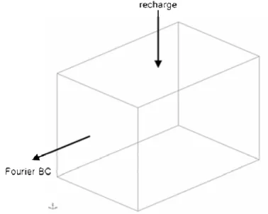
(23) Chapter 1. Introduction. 1.1 Context of the research Interest of end-users and policy makers for understanding and managing groundwater systems at the regional scale has increased for years. It appears clearly that water can not be managed internally within administrative local, regional or national boundaries but rather taking into account the physical boundaries of hydrological systems, such as hydrogeological limits for groundwater. This concern has been translated in the European Water Framework Directive (2000/60/EC) that states that water has to be managed at the scale of the Hydrographic District. This Directive introduces also the concept of “groundwater body” as the basic unit for groundwater management. The Directive states that a “good quantitative and qualitative status” has to be achieved for the year 2015. Moreover, upward trends of anthropogenic pollution have to be identified and reversed. Modelling tools simulating groundwater processes at the groundwater body scale are useful tools to help managers to implement the Directive. Such models can be used to improve the understanding of the functioning of groundwater systems and for predictions about the state of the system under defined pressures such as for example, climate changes and/or diffuse pollutions, among which nitrate has been identified as one of the most problematic and widespread diffuse contaminants of groundwater. Efforts are thus needed to develop regional scale groundwater models to assess with reliability the impact of land-use and related pollution on groundwater or to define appropriate long term management scenarios assessing the costs of such scenarios. At regional scale, groundwater models of different complexity, ranging from black-box models to physically-based and spatially-distributed models, have been used in various hydrogeological conditions. Black-box models, such as transfer functions, have been applied for example to model groundwater in large scale hydrological models, to model karstic systems, in particular for the interpretation of isotopic data. Their concepts are simple and attractive because they require relatively few data. The main drawbacks are however that modelling results are not spatially-distributed and their predictive capability is questionable, due to the semi-empirical nature of process descriptions. On the contrary, due to a more advanced description of ongoing processes, physically-based distributed models are expected to have better predictive capabilities than black-box models. However, because such models require more data, they are generally applied in case studies that are better characterised from. 21.

(24) Chapter 1. Introduction a hydrogeological point of view, for which the distribution of groundwater levels or solute concentrations in the groundwater systems are needed. The Hydrogeology Group of the University of Liège develops, for years now, regional groundwater models that were mainly focused until the beginning of this century on groundwater flow modelling. To face problems caused by the development of large scale groundwater model, a new flexible modelling approach, the Hybrid Finite-Element MixingCell method (HFEMC), has been developed in the framework of this thesis by the Hydrogeology Group of the University of Liège. This approach has been used in the framework of the research projects PIRENE and AquaTerra.. 1.2 The PIRENE and AquaTerra projects This research has been performed in the scope of two projects, the PIRENE and the AquaTerra projects which both aim to provide tools for integrated water management at the basin scale. In 2001, the Government of the Walloon Region (Belgium) initiated the PIRENE project to develop tools for integrated water quantity/quality management in the Walloon region. As a partner of this project, the Hydrogeology Group of the University of Liège had to develop a physically based, transient groundwater flow and transport model for the Walloon part of the Meuse Basin (approximately 18.000 km²). A methodology (the Hybrid Finite Element Mixing Cell Approach) and a numerical code grouping together different approaches (non-distributed or distributed mixing cells, advection-dispersion equation…) and allowing the transition from a simplified approach to a deterministic model were developed. This new methodology was tested on the Walloon part of the Meuse basin for which a groundwater flow model was developed. AquaTerra is an integrated project of the 6th EU RTD Framework Program grouping together scientists from 45 European (including Swiss and Serbian) organisations. It aims to provide a better understanding of the river-sediments-soil-groundwater system as a whole by identifying relevant processes, quantifying the associated parameters and developing numerical models to identify adverse trends in soil functioning, water quantity and quality. In this project, the Geer basin was used as a case study to test tools for groundwater trends analysis and to compare regional scale modelling approaches developed among other by the Hydrogeology Group of the University of Liège. 22.

(25) Chapter 1. Introduction. 1.3 Objectives of the research The two main objectives of this work are: •. to develop a general methodology for groundwater flow and solute transport assessment and modelling at the regional scale, in the framework of the European Water Framework Directive;. •. to perform, as a first test, an application of this methodology to assess and predict spatially-distributed nitrate trends in the Geer basin.. To reach the first objective of this research, a new flexible modelling approach, the Hybrid Finite Element Mixing Cell approach (HFEMC) has been developed. This approach allows combining in a single model, and in a fully integrated way, different mathematical approaches of various complexities for groundwater modelling in complex and large scale environments. This method has been implemented in the groundwater flow and solute transport numerical code SUFT3D. To reach the second objective, new field surveys, consisting in groundwater sampling for environmental tracer analysis, were performed to better understand the spatial distribution of the nitrate contamination before modelling. This document is structured as follow: In the second chapter, existing regional approaches to model groundwater are reviewed with their main advantages and drawbacks highlighted. Information about nitrate, environmental tracers and statistical trend analysis are also provided. The third chapter presents the HFEMC approach and the basic concepts underlying its implementation in the SUFT3D simulator. Synthetic tests developed to validate the approach and the implementation are exposed. In the fourth chapter, the Geer basin case study is presented. Main results of previous studies are synthesised. A recent study focusing on the link between nitrate contamination and the age of groundwater is also presented. Main results are presented and explanations concerning the spatial distribution of the nitrate contamination are proposed. The groundwater model developed for nitrate trends prediction is presented. Results of this model are discussed. A. 23.

(26) Chapter 1. Introduction socio-economic study of the impact of the nitrate contamination in the Geer basin in which the results of the model have been used is described as an example of use of regional scale groundwater model. Chapter 5 summarises the main conclusions of this work and presents future perspectives.. 24.

(27) Chapter 2. Review of the literature. 2 REVIEW OF THE LITERATURE. 25.

(28) Chapter 2. Review of the literature. 26.

(29) Chapter 2. Review of the literature. 2.1 Representative Elementary Volume The development of hydrogeologic models is based on a continuum assumption (Bear 1972; Eaton 2006 among others), flow and transport are considered on a volumetric averaged basis at a macroscopic scale assumed to be equivalent to an ideal porous media. The parameters governing flow and transport equations are defined at a scale larger than that of the microscopic pores. The minimum volume over which the governing equations of flow and transport apply is commonly referred to as a Representative Elementary Volume (REV) (de Marsily 1986; Bear and Verruijt 1987). The dimensions of such a REV are defined according the purpose of the investigation, but it must be of a size range within which values of parameters are statistically significant, more or less constant, continuous and large enough for parameters to be quantified experimentally. Representative Elementary Volumes used for groundwater flow problems are generally larger than those that should be used for the transport problem. Heterogeneities that are generally averaged in the flow problems have much more impacts when considering the solute transport problem (de Marsily et al. 2005).. 2.2 Migration of solutes in groundwater In the framework of this thesis, contaminants that will be considered are solutes only, defined here as a substance present in the water phase at a concentration below the solubility constant of that product in water. Pollutants present as a pure product or in a gaseous phase will not be considered in this study. Moreover, the considered solute is assumed to be at a concentration low enough to have a negligible impact on the density and viscosity of water. Processes considered in hydrogeology to model the transport of dissolved contaminants are (1) advection, (2) dispersion, (3) degradation and (4) retardation and trapping.. 27.

(30) Chapter 2. Review of the literature. 2.2.1 Advection Advection is the mechanism carrying contaminants in the porous media at the mean effective velocity of groundwater. The advective flux can be expressed by: f c = C v = C v D / θ m = −C K ∇h / θ m. (2.1). where f c is the advective flux [ML-2T-1]; C is the volumic concentration of contaminant [ML-3]; v is the mean velocity of solute migration, often called advective velocity or effective velocity [LT-1]; v D is the Darcy flux [LT-1]; θ m is the effective porosity, the proportion of the media accessible to the groundwater flow [-]; K is the hydraulic conductivity [LT-1]; h is the pressure potential [L]. The evaluation of the advective component of the solute transport requires determining the value of the hydraulic conductivity and of the effective porosity of the medium at the appropriate scale. Numerous authors have highlighted the scale dependence of the hydraulic conductivity values (Clauser 1992; Neuman 1994; Sánchez-Vila et al. 1995; Sánchez-Vila et al. 1996 among others). For example, Clauser (1992) synthesised values of permeability measured at different scales ranging from laboratory data to packer tests, Lugeon tests and calibration of models in crystalline rocks (Figure 2.1). An increase in average permeability of around three orders of magnitude from the laboratory to the borehole scale is clearly observable. Such an increase is not as well observable when going from the borehole to the regional scale. Permeabilities and thus hydraulic conductivities tend to increase with the characteristic scale of their measurement.. 28.

(31) Chapter 2. Review of the literature. Figure 2.1. Permeability of crystalline rocks and characteristic scale of measurements: bar marks the maximum permeability range when several individual values are reported; stars represent single values (from Clauser 1992). Renard (1996) proposed a synthesis of terminology used to define the scale of work in hydrogeology and the types of measurement used at these different scales. As shown in Figure 2.2, pumping tests which are one of the main tools used to determine hydraulic conductivities in subsurface hydrogeology are generally representative at a scale of maximum several hundreds of meters. Value of hydraulic conductivities determined by pumping tests can thus be considered as representative of REV of such a size.. Figure 2.2. Different scales and measurement techniques for studying porous media (modified from Renard 1996). 29.

(32) Chapter 2. Review of the literature The amplitude and physical meaning attributed to the effective porosity are function of the size of the REV. For example, in fractured media, if a REV of the size of the fracture is considered, a very high value for the porosity and the hydraulic conductivity will be obtained in the fissures. On the contrary if the fissures are not represented explicitly but assumed to be integrated in the properties of a REV of bigger size, the effective porosity will be smaller. The hydraulic conductivity obtained for this REV will also be smaller as it integrates the permeability of the fissures but also of the matrix. Hallet (1998) proposed the notion of REV porosity as being the mean effective porosity for the considered REV in fractured media. Brouyère (2001) noticed that values of the effective porosity deduced from tracer tests performed at Hermalle-sous-Argenteau in the alluvial aquifer of the Meuse river (Belgium) seem to increase slightly with the tracing distance and the modal travel time of tracers in the underground. Guimerà and Carrera (2000) synthesised data from different tracer tests in different fractured media (Figure 2.3). They noticed a significant correlation between peak arrival times and porosity values deduced from the interpretation of tracer tests. They assume that the portion of voids actually accessed by the tracer increases with time as a result of tracer diffusion into both the rock matrix and stagnant groundwater.. Figure 2.3. Travel time and apparent thickness porosity values for peak concentration arrival times (from Guimerà and Carrera 2000). 30.

(33) Chapter 2. Review of the literature. 2.2.2 Hydrodynamic dispersion Hydrodynamic dispersion results from the spreading of solutes around the mean advective position, caused by a combination of two processes (Figure 2.4): •. mechanical dispersion due to the distribution of the velocity around the mean value defined on the REV, fluctuations in space of the streamlines around the mean direction of flow and mainly heterogeneity not taken into account in the REV;. •. diffusion contaminant from zones of high concentrations to zones of lower concentrations.. The hydrodispersive flux can be expressed, with a Fickian law by:. f D = Dh ∇C. (2.2). where f D is the hydrodispersive flux [ML-2T-1]; C is the volumic concentration of contaminant [ML-3]; Dh is the tensor of hydrodynamic dispersion [L2T-1] that is equal to:. Dh = Dm I + D. (2.3). where Dm is the diffusion coefficient in the porous media [L2T-1]; I is the unity tensor; D is the tensor of mechanical dispersion [L2T-1]. If the axes are chosen in such a way that the x axis coincides with the direction of the average velocity (Frenet referential), the tensor D can be expressed by:. ⎡α L v ⎢ D=⎢ 0 ⎢⎣ 0. 0. αT v 0. 0 ⎤ ⎥ 0 ⎥ α T v ⎥⎦. (2.4). where α L and α T are respectively the longitudinal and lateral dispersivity coefficients [L], v is the magnitude of the velocity vector [LT-1].. 31.

(34) Chapter 2. Review of the literature. Figure 2.4. Spreading due to mechanical dispersion (a, b) and molecular diffusion (c) (Bear and Verruijt 1987).. It is also well known that dispersivity coefficients are scale dependant. For example, Gelhar et al (1992) synthesised dispersivity values obtained at different test sites. Data indicate a systematic increase of the longitudinal dispersivity with observation scale (Figure 2.5).. Figure 2.5. Longitudinal dispersivity versus scale of observation identified by type of observation and type of aquifer. The data are from 59 field sites characterized by widely differing geologic materials (Gelhar et al. 1992).. 32.

(35) Chapter 2. Review of the literature. 2.2.3 Degradation Chemical, biochemical or physical processes that produce the disappearance of the solute (and eventually producing other derived solute compounds) are grouped together under the notion of degradation. The simplest way to consider degradation is to take it into account through an equation of radioactive decay: ∂C = −λ C ∂t. (2.5). where λ is the first-order linear degradation coefficient [T-1].. 2.2.4 Retardation and trapping Retardation effects can be divided into two major categories (Brouyère 2001): •. chemical retardation, including all physico-chemical reactions between the solute and the porous medium;. •. physical retardation or dual-porosity effects.. Sorption group together different processes such as adsorption-desorption, absorption and cation exchange, that are dependant of the physico-chemical nature of the solute. It refers to mass transfer processes between the contaminants dissolved in groundwater and the contaminant sorbed on the porous media. It is often assumed that equilibrium conditions exist between the aqueous phase and the solid phase concentrations and that the sorption reaction is fast enough in comparison to the velocity of groundwater to be treated numerically as instantaneous. Different types of equilibrium controlled sorption isotherms are proposed in the literature (linear, Freundlich and Langmuir isotherms). The simplest relation expresses a linear sorption isotherm, which considers that the sorbed concentration C sorb is directly proportional to the solute concentration: C sorb = K d C. (2.6). where K d is the distribution coefficient [L³M-1]. Physical retardation processes affect all the solutes transported in the porous medium. Physical retardation mainly depends on the heterogeneity of the aquifer, solutes being trapped in less permeable parts of the aquifer (micropores, silty and clayey lenses, dead-end pores…). 33.

(36) Chapter 2. Review of the literature The dual-porosity concept, introduced by Coats and Smith (1964) following the failure of the advection-dispersion model to represent solute transport in heterogeneous media, considers two domains of porosity respectively mobile and immobile (or much less mobile). In chalk aquifers, immobile water is assumed to represent groundwater in the matrix, while the mobile water is associated to groundwater present in the fissures (Biver 1993; Hallet 1998; Brouyère 2006). Advection and dispersion take place only in the mobile zone, while chemical retardation can occur in both zones, although not necessary at the same rate. Diffusion is generally considered as the main process controlling the transfer of solutes from one zone to the other one. Mass conservation equation applied to the immobile domains can be expressed using a first order coefficient by:. θ im. ∂C im = α (C m −C im ) − λθ im C im ∂t. (2.7). where α is the first-order transfer coefficient between mobile and immobile water [T-1]; θ im is the immobile porosity [-]; θ m is the effective mobile porosity [-]; C m and C im are respectively the solute concentration in the mobile and immobile water [ML-3]; λ is the firstorder linear degradation coefficient [T-1]. Brouyère (2001) analysed the parameters obtained by the interpretation, considering interaction between mobile and immobile water, of different tracer tests performed in the aquifer of the alluvial plain of the Meuse river at Hermalle-sous-Argenteau. He noticed that an increase in the tracing distance, the modal transit time of the tracer and the modal effective porosity do not seem to affect the interpreted values of immobile porosity. On the contrary, he found that the transfer coefficient between the mobile and immobile water is clearly affected by scale and temporal effects. It decreases as a function of the tracing distance and of the transfer modal transit time and increases as a function of the modal effective velocity (Figure 2.6).. 34.

(37) Chapter 2. Review of the literature. Figure 2.6. Evolution of the transfer coefficient as a function of the tracing distance, the modal transit time and the modal effective velocity (modified from Brouyère 2001).. 35.

(38) Chapter 2. Review of the literature. 2.2.5 Solute transport equations Regrouping the different processes described here above, the solute transport equation can be written:. θm. ∂C m = −∇.(v D C m ) + ∇.(θ m D h ∇C m ) − λ θ m C m − α (C m − C im ) + q (C ′ − C m ) ∂t. (2.8). where θ m is the effective mobile porosity [-]; C m and C im are respectively the solute concentration in the mobile and immobile water [ML-3]; t is the time [T]; v D is the Darcy’s flux [LT-1]; Dh is the hydrodynamic dispersion [L2T-1]; λ is the linear degradation coefficient [T-1]; q are the volumetric fluxes associated to the source and sink [T-1]; C ′ is the concentration associated to these sources [ML-3].. 2.3 Existing approaches for modelling solute transport in groundwater at the regional scale Solute transport in groundwater is generally conceptualised using the different processes described in the previous section. At the regional scale, the acquisition of the relevant data and the development of solute transport models in groundwater remains a challenge. Generally speaking, existing conceptual and mathematical approaches used to model contaminant transport at large scale can be grouped into three main categories: transfer function approaches, compartment models and models relying on advanced solution of the advection-dispersion equation, in function of the way the different processes are taken into account or represented.. 2.3.1 Transfer function models Transfer function models, sometimes referred to as “black-box” or “lumped parameters” models, are usually used for the interpretation and correlation of datasets at the entry and outlet of the underground system (e.g. recharge and discharge zones). Transfer functions can be obtained through deconvolution of available time series when the structure and the functioning of the system are unknown. They can also be expressed as more or less elaborated parametric mathematical equations (e.g. Jury et al. 1982a; Amin and Campana 1996; Skaggs et al. 1998; Stewart and Loague 1999). Such approaches are relatively simple and they require. 36.

(39) Chapter 2. Review of the literature a limited number of parameters to be assessed. However, they provide a relatively low accuracy and because these models rely on integral mass balance formulations relating mass flux and concentrations at the system entry and output, the detailed spatial distribution and time evolution of concentrations within the underground system remain unknown. Such approaches have been mostly applied to isotopic and environmental tracer data (e.g. Duffy and Gelhar 1986; Ritzi et al. 1991; Maloszewski and Zuber 1996). This type of model can be expressed mathematically by the following convolution product: Y (t ) = F (t ) ∗ X (t ). (2.9). where X (t ) is the input function or the solicitation of the system; Y (t ) is the output function or the response of the system; F (t ) is the transfer function or impulse response. Transfer function approaches proposed in the literature differ essentially one from another by the way of representing and computing the transfer function F (t ) . Applied to solute transport through aquifers, Equation (2.9) becomes: ∞. C out (t ) = ∫ C in (t − τ )g (τ )dτ. (2.10). 0. where C out (t ) is the temporal evolution of concentration at the outlet of the aquifer system; C in (t ) is the temporal evolution at the entry of the aquifer system; τ is the time of entrance. of the solute in the system and t − τ the transit time; g (τ ) is the impulse response of the system whom the mathematical formulation depends on the mathematical model considered to represent the behaviour of solute moving in the system. If degradation is considered, Equation (2.10) becomes: ∞. C out (t ) = ∫ C in (t − τ ) g (τ ) exp(− λτ ) dτ. (2.11). 0. where λ is the degradation rate of the tracer and g (τ ) is the impulse response of the system.. 37.

(40) Chapter 2. Review of the literature 2.3.1.1 Non-parametric transfer functions. A non-parametric transfer function is not explicitly described by a function or a mathematical model. It is obtained by deconvolution of the system response Y (t ) by the solicitation X (t ) applied to the system. Long time series of data at the entry and outlet of the system are thus required to establish the transfer function F (t ) for that system. This form of the transfer function is static and the system is assumed to be perfectly linear and invariant. Skaggs et al. (1998) proposed an algorithm for the deconvolution that allow determining the nonparametric transfer function for 1D solute transfer across soil based on concentrations measured at the entry and outlet of the soil column. They concluded that one of the limits of such formulations is the impossibility to generalise the result to, for example, other soil thicknesses. 2.3.1.2 Transfer functions based on empirical or physical mathematical models. Such transfer functions are based on more or less complex mathematical equations, including a few parameters used to adjust the model from measurements of the stresses and responses of the system. Such transfer functions require time series of data long enough to adjust the parameters. Due to the large set of mathematical functions that are available, it is theoretically possible to consider non-linear or time-variant systems. Jury (1982b) proposed a log-normal function to represent the distribution of transit times (indeed the transfer function) of solutes through soils. The transfer function can also be based on a physical model, for example an analytical solution of the advection-dispersion equation that allows the evaluation of the distribution of transit times in the medium (Jury and Roth 1990; Roth and Jury 1993). Stewart and Loague (1999) proposed a generalization of the works of Jury (1982b) at large scale by introducing the notion of type transfer functions. The advantages of such approaches are mainly their simplicity and the limited number of required parameters. Their main drawback is the low precision that they provide and, above all, the fact that such models give information on the concentrations and mass fluxes at the outlet of the system but not on the spatial distribution of the concentrations inside the system. For example, the application of a transfer function aiming to represent the transit of a contaminant from agriculture to the river network, through the underground, allows estimating the mass flux associated to groundwater discharge but does not give information on the spatial distribution of the contaminant inside the aquifer.. 38.

(41) Chapter 2. Review of the literature In most cases, the transfer functions are characterised by one or two unknown parameters determined solving the inverse problem. Different codes have been developed to solve such inverse problems selecting different kinds of transfer functions, e.g. FLOWPC (Maloszewski and Zuber 1996), TRACER (Bayari 2002), LUMPED (Ozyurt and Bayari 2003). Different authors have proposed syntheses of the main existing models and applications generally based on the use of these models for the interpretation of isotopic or environmental tracer data (Maloszewski and Zuber 1982; Duffy and Gelhar 1985; Duffy and Gelhar 1986; Ritzi et al. 1991; Maloszewski and Zuber 1996; Maloszewski et al. 2004 among others). A summary of most common mathematical models used in transfer functions is presented hereafter. 2.3.1.2.1 Perfect mixing model. The perfect mixing model relies on the assumption of perfect mixing of solutes within the considered reservoir. This implies that any solute entering the system is instantaneously and completely mixed with the entire volume of groundwater and solute already present in the aquifer reservoir. The concentration at the outlet of the system is assumed to be equal to the mean concentration within the reservoir. Knowing the concentration at the outlet of the system, it is theoretically possible to know the mean concentration within the aquifer. The transfer function representing perfect mixing can be mathematically expressed by:. g (τ ) =. 1 ⎛ τ⎞ exp⎜ − ⎟ T ⎝ T⎠. (2.12). where g (τ ) is a function of the distribution of the transit time in the aquifer; T is the mean. transit time of water in the underground. In regards to the mathematical formulation of the function representing the model, it is often also called exponential model. This model is, for example, applicable when the groundwater sampling induces a mixing of groundwater with different travel times (Figure 2.7).. 39.

(42) Chapter 2. Review of the literature. Figure 2.7. Situation for which the mixing model is applicable (modified from Maloszewski and Zuber 1982). 2.3.1.2.2 Piston-flow model The piston-flow model assumes that solutes move from the entry to the outlet of the system by a purely advective process, introducing simply a delay corresponding to the travel time within the aquifer. This model assumes thus that the solute travel time between the entry and the outlet of the system is equal for all the stream lines and that mechanisms of dispersion and molecular diffusion are negligible. Mathematically, the transfer function representing pistonflow can be expressed by: g (τ ) = δ (τ − T ). (2.13). where g (τ ) is a function of the distribution of the travel times in the aquifer; T is the mean transit time of water in the underground. The piston-flow model is, for example applicable, neglecting the dispersion in the case of a confined aquifer with a recharge zone limited in space and located far away from the pumping wells (Figure 2.8).. Figure 2.8. Situation for which the piston-flow model is applicable (modified from Maloszewski and Zuber 1982). 40.

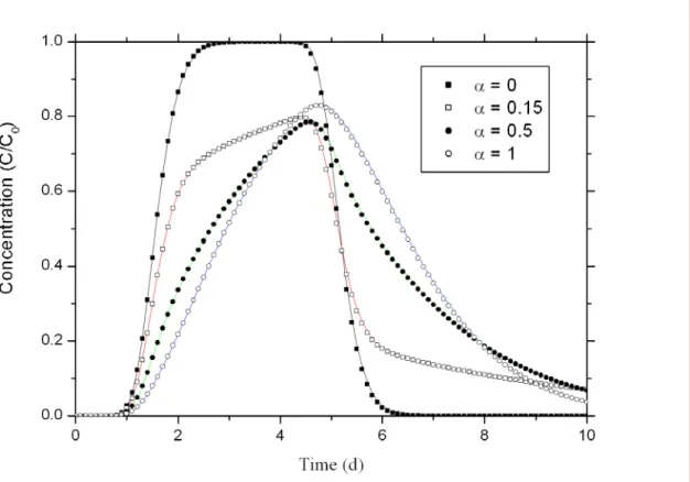
(43) Chapter 2. Review of the literature. 2.3.1.2.3 Dispersion model The dispersion model links concentrations at the entry and the outlet of the system by a transfer function based on a simplified analytical one-dimensional solution of the advectiondispersion equation. Mathematically, the transfer function representing the dispersion model can be expressed by:. g (τ ) =. 1. ⎛ (1 − τ T )2 ⎞ ⎟ exp⎜⎜ − ⎟ P T τ 4 τ D ⎝ ⎠ 1. 4π PD τ. T. (2.14). where PD is the dispersion parameter reflecting the relative importance of the dispersion processes to the advection processes. This parameter is the inverse of the Peclet number which is the ratio between advection and dispersion and which is defined for a flow parallel to the direction x by:. Pe =. v x ∆x ∆x = Dx αL. (2.15). Where Pe is the Peclet number [-]; v x is the advective velocity in the x direction [LT-1]; ∆x is the cell dimension in the x direction [L]; D x is the xx component of the dispersion tensor [L2T-1]; α L is the longitudinal dispersivity [L]. This model is applicable when dispersion process can not be neglected. Maloszewski (1994) showed that, for dual-porosity media, the dispersion model is usable when the travel time T is larger than 2-3 years. However, the application of the dispersion model to dual-porosity media yields to determine an apparent mean travel time T * instead of the real travel time of groundwater T. This apparent mean travel time T * can be expressed by: ⎛ θ + θ im T * = ⎜⎜ m ⎝ θm. ⎞ ⎟⎟ T = RT ⎠. (2.16). where T* is the apparent mean travel time of groundwater [T]; θ m is the effective mobile porosity [-]; θ im is the immobile water porosity [-] ; T is the real mean travel time [T] and R is the retardation factor resulting from the diffusion of tracer into stagnant water [-].. 41.

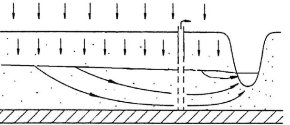
(44) Chapter 2. Review of the literature 2.3.1.2.4 Combined models In the models mentioned here above, only one fitting parameter is generally considered. To model real cases, it is often necessary to have a greater flexibility for the calibration of the transfer functions with observed time series of concentrations. Several authors have thus proposed more elaborated models based on the combination of simple models. Amin and Campana (1996) proposed a general model from which, by fixing in a appropriate way the parameters, it is possible to infer most of the models cited here above, as well as several combinations of these models. One generalisation of the approaches presented here above is the example of the combined exponential – piston-flow model. This model includes a parameter called mixing efficiency that allows for the continuity from the piston-flow model (corresponding to a mixing efficiency equal to zero) to the exponential model (corresponding to perfect mixing with a mixing efficiency of 1). Mathematically, the transfer function representing the combined exponential – piston-flow model can be expressed by:. ⎞ ⎛ ητ exp⎜ − + η − 1⎟ T ⎝ T ⎠ g (τ ) = 0 g (τ ) =. η. for τ > (η − 1)T / η. (2.17). for τ ≤ (η − 1)T / η. (2.18). where η is the mixing efficiency. This model is, conceptually, applicable to unconfined aquifers with a thick unsaturated zone (Figure 2.9). The piston flow component of the combined model allows representing solute transport in the unsaturated zone and the exponential component transport in the saturated one.. 42.