The climate induced variation of the continental biosphere: A model simulation of the last glacial maximum

GEOPHYSICAL RF.,SEARCH

LETTERS, VOL. 19, NO. 9, PAGES 89%900, MAY 4, 1992

THE CLIMATE INDUCED VARIATION OF THE CONTINENTAL BIOSPHERE ' A MODEL SIMULATION OF THE LAST GLACIAL MAXIMUM

P. Friedlingstein•,a, C. Delire 2, J.F. Mtiller a and J.C. G•rard 2

Abstract. A simplified three-dimensional global climate model was

used

to simulate

the

surface

temperature

and

precipitation

distributions

for

the

Last

Glacial

Maximum

(LGM), 18 000 years

ago.

These

fields

were

applied

to a bioclimatic

scheme

wict•

parameterizes

the

distri-

bution

of eight

vegetation

types

as a function

of biotemperature

and

annual

precipitation.

The model

predicts

a decrease,

for LGM com-

pared

to

present,

in lorested

area

balanced

by

an

increase

in desert

and

of vegetation

based

on palcodata.

However,

the

estimated

biospheric

carbon content (phytomass and soil carbon) at LGM is less reduced than in the reconstructed one. Possible reasons for this discrepancy are discussed.

Introduction

Analysis

of air bubbles

in ice cores

has

clearly

established

that

the atmospheric

concentration

of carbon

dioxide

during

the Last

the

preindustrial

(interglacial)

level. A larger

content

of carbon

in

the terrestrial biosphere during glacial periods could be a possible cause of this low atmospheric CO2 concentration. Transfer of carbon

from

the

biosphere

to the atmosphere

could

thus

explain

the

rise

in

atmospheric

CO,.,

concentration

between

LGM and

the

preindustrial

Using

a general

circulation

model

and

a bioclimatic

scheme,

Pren-

tice

and

Fung

(1990)

estimated

that

the amount

of carbon

in the

veg-

interglacial.

They

found

that

200 Gt of carbon

were

stored

by veg-

This

additional

carbon

pool

at LGM has

almost

e•actly

counterbal-

the

present

land

area.

They

concluded

that

carbon

transfer

between

the

biosphere

and

the atmosphere

should

not

have

been

a dominant

factor

in the

large

atmospheric

CO,•

level

change

between

glacial

and

interglacial

events.

In contrast,

Adams

et al. (1990),

basing

their

estimates

on palynological,

pedo!ogical

and

sedimentological

data,

been smaller by more than 1000 Gt of carbon at LGM than during the Holocene, corresponding to a doubling in the terrestrial carbon content from LGM to present interglacial. This result has important implications on the ability of the ocean to store the large amounts of carbon that may have been transfered to the atmosphere-biosphere system since the LGM. The contrast between the two sets of results

was

already

present

in the reconstruction

they

made

of the

vegetation

vegetation

types

having

a low carbon

storage

per unit area,

such

as

they are currently. Moist climate types (with high carbon storage)

were

almost

absent

from

the large

areas

which

they

occupy

today.

In

contrast,

following

the

simulation

made

by Prentice

and

Fung

(1990),

the

driest

vegetation

types

would

have

covered

a smaller

area

than

today.

The

aim

of this

study

is to simulate

the

climate

and

the

distribution

of vegetation

types

at LGM and

to compare

it to the

reconstruction

• Universit•

Libre

de Bruxelles,

2 Institut

d'Astrophysique-

Universit•

de Liege, :• Institut d'AGronomie Spatiale - Bruxel!es

Copyright

1992

by the American

Geophysical

Union.

Paper

number

92GL00546

0094-85 34/92/92GL-005 4 6503,00

made

by Adams

et al. Discrepancies

between

this

work

and

that

of

The atmospheric

model

and the bioclimatic

scheme

climate

model

developed

by Sellers

(1983,

1985).

Description

of this

model and discussion of its ability to reproduce the present climate

can

be found

in the

original

papers.

Most

of the

major

features

of the

sea

level

pressure

and

temperature

fields

are

quite

well

simulated.

As

some

discrepancies

with

the observed

field. For

present

conditions,

it yields

a global

average

sea

level

temperature

of 289.6

K and

total

An empirical

model

of the

biosphere

has

been

developed.

It pre-

dicks

the

global

distribution

of the

vegetation

types

and

the

main

car-

bon

pools

and

fluxes

from

two

climatic

variables:

the

annual

precipi-

tation

and

the

biotemperature

(the

biotemperature

is the

mean

annual

temperature

(in øC)

considering

only

positive

monthly

temperatures).

Starting

from

the

World

Ecosystem

Database

of Olson

et al. (1985)

which

includes

52 ecosystems

on a 0.5øx 0.5

ø resolution

grid,

we de-

fine

eight

broad

vegetation

types

(numbers

in parenthesis

refer

to Ol-

son's

classification):

perennial

ice (17,69-71),

desert

and

semi-desert

(49-51),

tundra

(53,63),

coniferous

forest

(20-23,57,60-62),

deciduous

forest

(24-26,

46,48,56),

grassland

and

shrubland

(4042,47,52,59,64),

seasonal

tropical

forest

(27,28,32,43)

and

evergreen

tropical

forest

(29,33).

Present-day

5øx 5* annual

precipitation

and

biotemperature

of precipitation

(Shea,

1986)

and

surface

temperature

(Trenberth

et

al., 1988).

The relationship

between

the spatial

distribution

of each

vegetation

type

and

the two climatic

variables

was

then

determined

empirically.

Each

vegetation

type

is allowed

to exist

within

a defined

domain

of precipitation

and

biotemperature

(Table

1). The

vegetation

distribution

predicted

by this

bioclimatic

scheme,

for present-day

pre-

cipitation

and

temperature

fields,

agree

with Olson's

database.

The

compared

with the data,

particularly

in mountainous

regions.

Net

primary

productivity

(NPP),

phytomass

and

soil

organic

carbon

pool

fied

by expressing

NPP

as the minimum

value

of two functions,

the

first

depending

on mean

annual

precipitation

and

latitude,

the second

NPP = min

with

f/3•

= 69.1875xBT

if BT < 8 øC

•

err)) if BT > 8 øC

fe

= 1125.x(1.

- exp(-6.64x10-ax

P)) in the tropics

BT = P = NPP =

biotemperature expressed in øC

annual precipitation expressed in mm/y

net primary

production

expressed

in gC/m2/y.

The parameters

were

adjusted

to fit the global

NPP distribution

given

by Fung

et aI. (1983). The global

annual

NPP predicted

by

carbon in herbaceous and woody biomass in the different vegetation

types

derived

from

Goudriaan

et al. (1984). Values

adopted

are

study

(1982)

which

relates

this

variable

to biotemperature

and

annual

898

Fricdlingstein

et al.' Continental

Biosphere

at LGM

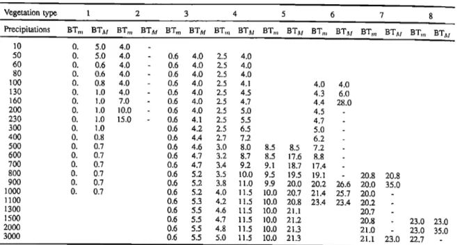
Table

1. Minimum

biotemperature

(BTm)

and

maximum

biotemperature

(BTam)

(in

øC)

for

different

annual

precipitation

levels

(in

mm/yr) allowing the existence of each vegetation type (refer to Table 2, Column 1).

Vegetation

type

1

2

3

4

5

6

7

8

Precipitations

_{BTm BTM BTm BT.sl BTm BT.4• BTm BT:u BT,, BT•u BT,, BT.w BTm BT:xj BT,n BT,w}

10 o. 5.0 4.0 - 50 o. 5.0 4.0 - 0.6 4.0 2.5 4.0 60 o. 0.6 4.0 - 0.6 4.0 2.5 4.0 80 0. 0.6 4.0 - 0.6 4.0 2.5 4.0 100 0. 0.8 4.0 - 0.6 4.0 2.5 4.1 130 0. 1.0 4.0 - 0.6 4.0 2.5 4.5 160 0. 1.0 7.0 - 0.6 4.0 2.5 4.7 200 0. 1.0 10.0 - 0.6 4.0 2.5 5.0 230 0. 1.0 15.0 - 0.6 4.1 2.5 5.5 300 0. 1.0 0.6 4.2 2.5 6.5 400 0. 0.8 0.6 4.4 2.7 7.2 500 0. 0.7 0.6 4.6 3.0 8.0 600 0. 0.7 0.6 4.7 3.2 8.7 700 0. 0.7 0.6 4.7 3.4 9.2 800 0. 0.7 0.6 5.2 3.5 10.0 900 0. 0.7 0.6 5.2 3.8 11.0 1000 0. 0.7 0.6 5.2 4.0 11.5 1100 0.6 5.3 4.2 11.5 ! 300 0.6 5.5 4.6 11.5 1500 0.6 5.5 4.7 ! 1.5 2000 0.6 5.5 4.8 11.5 3000 0.6 5.5 5.0 11.5 4.0 4.0 4.3 6.0 4.4 28.0 4.5 4.7 - 5.0 - 6.2 - 8.5 8.5 7.2 - 8.5 17.6 8.8 9.1 18.7 17.4 9.5 !9.5 19.1 9.9 20.0 20.2 26.6 10.0 20.7 21.4 25.7 10.0 20.8 23.4 23.4 10.0 21.1 10.0 21.2 10.0 2!.3 10.0 21.3 20.8 20.8 20.0 35.0 20.0 - 20.2 - 20.7 - 20.8 - 23.0 23.0 21.0 - 23.0 35.0 21.1 23.0 22.7 -

Glacial climate simulation

In order to simulate the climate of the Earth during the Last Glacial

Maximum, 18000 years ago, some input parameters and boundary conditions of the model were changed. The orbital parameters were

taken from Berger (1978). The atmospheric CO• concentration was decreased to 200 ppm, in agreement with the CO-., measurements from

the Vostok ice core (Bamola et al., 1987). Coastlines were modified

assuming a sea level drop of 130 m (Climap, 1976). Sea ice and snow cover were taken from Climap for February and August. Their annual

cycle was approximated by a sine function with February and August

values taken as extrema. The model was run to steady state for the

present day and the LGM conditions. The difference between the

simulated temperature field for the present and for the LGM was then added to the observed temperature field above mentioned. The same was done for the precipitation field. In this way, the simulated climate change was rooted in the observed climatology and the effect of the systematic errors of the model was minimized. In this simulation, the

global temperature and precipitation rates at LGM were decreased by

3.13 K and

0.35 mm/day

respectively.

The land

temperature

dropped

Africa and Australia.

The modeled

temperature

and precipitation

fields were then used to calculate the biotemperature and annual precipitation distributions. These two fields, simulated at a 10øx 10 o resolution, were linearly interpolated on a 5øx 5 ø grid and applied to the bioclimatic scheme described before.

Simulated glacial biosphere

Global maps of the simulated distribution o1' vegetation are pre-

sented in Figure 1. Following this simulation, the boreal vegetation types were shifted towards lower latitudes with tundra occupying ar-

eas presently covered by coniferous, and to a lesser extent, deciduous

forests. This is basically a result of the reduced temperatures over these regions. Lower precipitation rates 18 kyr years ago in Australia and Sahel explain why deserts were more extensive and grasslands and shrublands less extensive. Decreased precipitation was also responsi- ble for the reduction in seasonal tropical forests which are replaced

by grasslands and shrublands in Southern Africa. However, seasonal

tropical forests expanded on lands that are immersed today in South East Asia and Oceania. Evergreen tropical forests were almost absent from the equatorial regions where they are to be found now. As ev- ergreen tropical forests have high NPP, the reduction in their size has a strong negative effect on the total living phytomass at glacial time (Column 5, Table 2). Total living phytomass is also strongly depen-

dent on the redistribution of coniferous forest and tundra, since the

latter is much less carbon-productive than the former. On the other hand, additional phytomass (about 120 GtC) was present due to the

Table

2. Comparison

of the

extent

(in 10

'• km'2)and

carbon

content

(in GtC)

of the

terrestrial

biosphere

for present

naLural

and

LGM

conditions (Antarctica excluded).

Vegetation type Area Phytomass Soil carbon

Present LG M Present LG M Present LG M

1 Perennial ice 3 23 0 0 0 0

2 Desert and semidesert 16 24 1 I 31 34

3 Tundra 10 21 25 34 124 236

4 Coniferous forest 24 12 236 91 307 159

5 Deciduous forest 16 14 237 204 163 144

6 Grassland and shrubland 36 34 30 27 240 239

7 Seasonal tropical forest 20 25 225 276 236 312

8 Evergreen tropical forest 11 ' 6 147 64 196 103

Friedlingstein

et al. ß Continental

Biosphere

at LGM

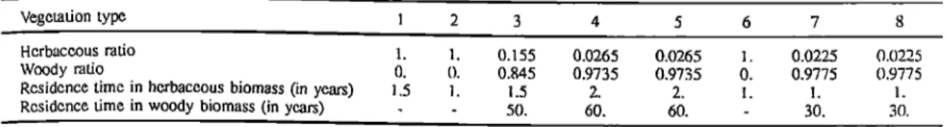
Table

3. Fractions

of herbaceous

and

woody

biomass

and

mean

residence

time

by

vegetation

type

(numbers

refer

to Table

2, Column

1).

Vegetation type 1 2 3 4 5 6 7 8

Herbaceous ratio 1.

Woody ratio 0.

Residence time in herbaceous biomass (in years) 1,5 Residence time in woody biomass (in years) -

1. 0.155 0.0265 0.0265 1. 0.0225 0.0225

0. 0.845 0.9735 0.9735 0. 0.9775 (1.9775

1. 1.5 2. 2. 1. 1. 1. - 50. 60. 60. - 30. 30.

larger

land

area

resulting

from tl•½

lower

sea

level. Altogether,

the

phytomass

accumulated

by the vegetation

at LGM was

23 % lower

before

does

not present

a significant

difference

between

the present

Discussion and conclusions

An interesting comparison is possible with the reconstruction by Adams et al. (1990). The general trends between the two approaches agree, showing an increase at LGM in the areas covered by low veg-

etation types and deserts at the expense of forests. The Adams et al. results are more drastic than those in our study: they estimated

a relative change of -52 %, +20 % and +98 %, with Antarctica, (

to compare with -20 %, +20 % and +136 % in the present study,

without Antarctica) for areas covered by forest, low vegetation types and deserts (Antarctica included), respectively. Due to this important shift from high to low carbon content vegetation types, the amount of terrestrial carbon at LGM is significantly smaller in their study. They estimated a total decrease of 1071 GtC (if wetlands and peat- lands are not considered), whereas we modeled a smaller drop of 300 GtC (Figure 2). Reasons for this diff'erence may probably be found in the simulated LGM climate, especially the precipitation field. Con- sistently with other atmospheric models (Rind, t987), the simplified model used here seems to overestimate the amount of water available for vegetation. Particularly, precipitation rates seem to be too high in

intra-tropical regions to curt off the forested areas as in the Adams's

study. To test this assumption, the annual precipitation field at LGM,

-60 90

-30 •---

- 60 - 180

Fig.

1. (a). Simulated

present

day

distribution

of vegetation

types:

perennial

ice [i], warm

desert

[w], grassland

and

shrubland

[g], tundra

[t],

900 Friedlingstein et al.' Continental Biosphere at LGM

ooo[ (b)

1000

::• phytomass

fJ•

soil

carbon

Fig. 2. Living phytomass and soil carbon content for prcscnt day

and LGM conditions: (a) this work, (b) Adams ctal. (1990) (without wetlands and peatlands).

estimated from January and July distributions simulated by the NCAR

CCM0 (Kutzbach and Guctter, 1986), was applied to the bioclimatic scheme. The resulting distribution of vegetation is similar to the one obtained with the simplified GCM, except for the equatorial regions where the presence of evergreen tropical forest as extensive as today

is simulated. This can be explained by the CCM0's steep gradient

of the precipitation field between the tropics and the equator, allow- ing large tropical deserts neighbouring important moist climate types around the equator. Excessive precipitation rates may also account

for the slightly larger carbon pool at LGM than today as estimated by

Prentice and Fung (1990).

Another limitation of both our and Prentice and Fung's study

results from the assumption that the bioclimatic scheme developed

for present climate remains valid for LGM conditions, i.e. the

hypothesis that precipitation and biotemperature are the dominant factors in tile vegetation "struggle for !il'e". Low atmospheric CO,_, content could further reduce the phytomass in a non negligible way. The productivity of the biosphere and hence the phytomass and the soil carbon at the LGM would be reduced by a factor of about two if the parameterization of the Osnabrfick model (Esser, 1987) was

used to take into account the "dcfertilization" CO._, effect. Moreover, the bioclimatic scheme assumes that the vegetation distribution is in

equilibrium with climate. Since the last glaciation lasted more than 10000 years, this equilibrium wits probably reached. But this may not

be the case when considering faster climate changes. Studies of the

vegetation distribution of the next century require a dynamical model

of vegetation including, among other factors, the role of soils.

Our results, i.e. a low biospheric carbon content at LGM, combined with the low atmospheric CO._, concentrati9n, suggest that the oceans should have played an important role in the carbon storage during the glacial to interglacial transitions, as also revealed by deep-sea core

analysis (Shackleton, 1983).

Acknowledgments. We thank Pr. W. Sellers Ibr his help in the use of the simplified Global Climate Model and P. Bchling for pro-

viding outputs of the NCAR CCM0 runs I'or LGM conditions. Useful discussions with, G. Brasscur, D. Erickson, H. Faurc, B. Holland and

R. Keeling are gratefully acknowledged. The authors are grateful

to the Belgian Institute for Encouragement of Industrial and Agri-

cultural Scientific Research (IRSIA) (PF and CD) and the Belgian

Fund for Scientific Research (FNRS) (JFM and JCG) for financial

support. Part of this work was supported by the Belgian National Im- pulse Programmes "Global Change." and "Information Technologies

- Supcrcomputing" of tile Belgian State - Prime Minister's Service Science Policy Office.

References

Adams, J.M., H. Faure, L. Faure-Denard, J.M. McGlade and F.I. Woodward, Increase in terrestrial carbon storage from the Last Glacial Maximum to the present, Nature, 348, 711-714, 1990. Bamola, J.M., D. Raynaud, Y.F. Korotkevich antl C. Lorius, Vost0k

ice

core

provides

160

000

years

record

of atmospheric

CO.,,

Nature, 329, 408-414, 1987.

Berger,

A., Long-tcm-•

variations

of daily insolation

and

quaternary

climate changes, J. Atmos. Sci., 35, 2362-2367, 1978.

Climap project members, The surface of tile ice-age Earth, Science, 191, 1131-1137, 1976.

Esser, G., Sensitivity o1' global carbon pools and 11uxes to human and

potential climatic impacts, ?kllus, 39 B, 245-260, 1987. Fung, I., K. Prentice, E. Matthews, J. Lerner and G. Russel, Three

dimensional model study of atmospheric CO2 response to sea-

sonal exchanges with the terrestrial biosphere. J. Geephys. Res., 88, 1281-1294, 1983.

Goudriaan, J. and P. Ketncr, A simulation study l'or the global carbon

cycle including man's impact on the biosphere, Clim. Change, 6, 167-192, 1984.

Kutzbach, J.E. and P.J. Guettcr, The influcnce of changing orbital parameters and surface boundary conditions on climate simula-

tions for the past 18 000 years, J. Atmos. Sci., 43, 1726-1759,

1986.

Lieth, H., Modeling the primary productivity of the world, in Primary

productivity of the biosphere, edited by Lieth, H., and R.H. Whittaker, pp. 237-263, Springer-Verlag, New York, 1975. Olson, J.S., J.A. Watts and L.J. Allison, Major world ecosystem com-

plexes ra.nked by carbon in live vegetation. A data base. ORNL-5862, Oak Ridge National L.aboratory, Oak Ridge, Tenn, 164 pp., 1985.

Post, W.M., W.R. Emanuel, P.J. Zinke and A.G. Stangenberger, Soil

carbon pools and world life zones, Nature, 298, 156-159, 1982.

Prentice K. and Fung I., The sensitivi.ty of terrestrial carbon storage to climate change, Nature, 346, 48-51, 1990.

Rind, D., Components of the ice age circulation, J. Geephys. Res., 92, 4241-4281, 1987.

Sellers, W., A quasi three dimensional climate model, J. Clim. Appl. Meteorel., 22, 1557-1574, 1983.

Sellers, W., The effect of a solar perturbation on a global climate

model, J. Clim. Appl. Meteorel., 24, 770-77.6, 1985.

Shackleton N.J., M.A. Hall, J. Line and Cang Shuxi, Carbon isotope data in core V19-30 confirm reduced carbon dioxide concen- tration in the ice age atmosphere, Nature, 306, 319-322, 1983. Shea, D.J., Climatological atlas: 1950-1979, NCAR Technical Note,

NCAR/TN-269 +STR, 1986.

Trenberth, K.E. and J.G. Olson, ECMWF global analyses 1979-1986:

Circulation Statistics and Data Evaluation, NCAR Technical

Note, NCAR/TN-300+STR, 1988.

P. Friedlingstein

and

J.F.

Mti!ler,

Institut

d',Adronomie

Spattale,

3,

C. Delire and J.C. G6rard, Institut d'Astrophysique, Universit0, de

Liege, 5, avenue de Cointe B-4000 Lib•ge- Belgium.

(received ß January 20, 1992;

revised' March 4, 1992;