Proceedings of the Summer Program 2012
Statistical inverse analysis and stochastic
modeling of transition
By O. Marxen†, G. Serino†, F. Pinna†,
P. Constantine, C. Gorle
A N DG. Iaccarino
A computational method is introduced to infer statistical information on boundary-layer perturbations upstream of laminar-turbulent transition in a supersonic boundary layer. The method uses the intermittency function as a basis, which specifies the amount of time a flow is turbulent at a given streamwise location. The methods yields a joint probability density function for amplitude and frequency of boundary-layer perturbations upstream of transition. It relies on linear stability theory to link the probability density function with the intermittency. In order to infer parameters governing the function, we perform a statistical inverse analysis using the Markov chain Monte Carlo method. The approach is applied to a synthetic test case and to experimental data.
1. Introduction
The knowledge of the location of laminar to turbulent transition is essential for nu-merous engineering applications. For a hypersonic vehicle, an accurate prediction of the transition location may allow to precisely define the dimensions of the vehicle’s thermal protection system. Transition does not only affect the performance of an atmospheric re-entry vehicle, it also plays a key role in the safety of the vehicle and its payload. The development of credible engineering models for the prediction of laminar-turbulent transition is therefore an important task.
The transition location depends on a large number of parameters and is, consequently, difficult to predict. In particular, perturbations in the boundary layer upstream of tran-sition are known to affect the trantran-sition process. Except in studies performed within a carefully controlled laboratory environment, transition is a highly random process due to its strong sensitivity to these perturbations. Instead of trying to determine fixed values of the most important governing parameters, in particular those relating to boundary-layer perturbations, we should characterize them in a statistical way in order to account for the stochastic nature of transition.
The laminar-turbulent transition process may be divided into three stages: receptivity, linear disturbance evolution and nonlinear breakdown to turbulence. Most transition modeling approaches are deterministic and rely on empirical data (Langtry & Menter 2009), but they do not capture the stochastic nature of the physical processes active during these stages. Only the nonlinear breakdown stage, including the formation of turbulent spots, has been modeled in a probabilistic way (Vinod & Govindarajan 2004; Pˇecnik et al. 2011).
† Aeronautics and Aerospace Department, von Karman Institute for Fluid Dynamics, Chauss´ee de Waterloo, 72, B-1640 Rhode-St-Gen`ese, Belgium
1.1. Controlled transition
Investigations with explicitly forced, controlled perturbations (Marxen et al. 2010) at low levels of freesteam turbulence are useful to advance our understanding of mechanisms involved in the laminar-turbulent transition process. These studies consider the so-called controlled deterministic transition. Laboratory experiments with such forcing have been successfully reproduced by means of numerical simulation (Mayer et al. 2011). However, an approach in which transition is caused by a limited number of forced deterministic perturbations may not be representative of the operating conditions of a vehicle. Using random forcing to introduce the disturbances responsible for transition is thus a logical alternative to account for the non-deterministic nature of transition (Marxen & Iaccarino 2009). The corresponding process, controlled random transition, is essentially the same as the controlled deterministic transition, except that the forcing is not deterministic: in both controlled random and controlled deterministic transition, the flow field is inten-tionally forced with one or multiple characteristic perturbations.
1.2. Natural transition
In many engineering applications, intentional forcing of boundary-layer perturbations is entirely absent. Yet, in these applications the flow will still transition to turbulence, and this situation is commonly called natural transition. At least in environments with low disturbance levels representative of free flight in the atmosphere, controlled and natural transition share a central feature: the transition process is typically governed by the convective amplification of high-frequency boundary-layer disturbances. Unlike for controlled transition, a commonly accepted way to numerically treat natural transition has not yet emerged.
One way to compute natural transition is to apply the numerical approach used for controlled random transition, but with the controlled forcing adapted to the operating conditions of interest. Specifically, all the disturbances naturally present in the flow field should result from the random forcing. An example for such a computation is given by Jacobs & Durbin (2001), who use the continuous modes of the Orr-Sommerfeld and Squire equations. In order to represent freestream turbulence, they have chosen an amplitude distribution for these modes which corresponds to homogeneous isotropic turbulence, with uniformly distributed random phase angles.
Such an approach requires a good a priori statistical characterization of the natural disturbance spectrum upstream of the transition location, i.e., a statistical description of frequencies, wave lengths, amplitudes and relative phase differences. Unfortunately, boundary-layer perturbations are difficult to measure and are usually not sufficiently well characterized experimentally. On the other hand, the region of laminar-turbulent transition is often fairly well documented in the form of skin-friction coefficients or heat transfer at the wall. Our objective is to evaluate whether a statistical inverse analysis, using, for example, measured heat-transfer coefficients as a basis, offers the possibility to provide a characterization of relevant disturbance spectra upstream of the transition zone.
1.3. Transition modeling and linear stability theory
The numerical methods used in the references cited in sections 1.1 and 1.2 are compu-tationally too expensive for transition modeling in practice. Simplified methods able to link boundary-layer perturbations upstream with transition downstream are therefore required. Today’s state-of-the-art transition models provide a deterministic, fixed
tran-sition location. Two commonly used classes of methods are correlation-based methods and the eN-method.
Correlation-based methods (Reda 2002) rely on an averaging of empirical data and may provide a confidence interval based on the root-mean-square value of the averaged data. Relevant parameters require tuning in order to match available experimental data. For example, Serino et al. (2012b) applied a two-equation transition model in their computa-tion based on the Reynolds-averaged Navier-Stokes equacomputa-tions and varied the freesteam turbulence level until the transition onset location matched the experimental one.
Linear stability theory (LST) for compressible boundary layers (Mack 1969) is a fairly accurate way to capture the stage of linear disturbance evolution by computing the local growth rate of boundary layer perturbations. It is based on the linearized Navier-Stokes equations together with a parallel-flow assumption. The eN-method, which has been
applied to supersonic boundary layers by Malik (1989), considers the integrally most amplified disturbance from LST to yield the transition onset location. Typical N -factors at transition onset (Malik 2003) lie in the range of 5 − 10.
Both the receptivity and the nonlinear stages are only indirectly considered in the eN
-method by choosing a so-called critical value for N : this value, Ncrit, hence collectively
represents the physical mechanisms active in the receptivity and nonlinear stages. In setups with a high level of freesteam turbulence or significant surface roughness, the level of boundary layer perturbations at the end of the receptivity stage is expected to be high. This is reflected by choosing a small Ncrit. Regarding the nonlinear stage, the
standard eN-method assumes that transition is caused by the linear disturbance which
is integrally most amplified and reaches the critical N -factor first, independent of the underlying amplification mechanism.
2. Method
In the following, we consider the self-similar boundary layer developing in the stream-wise direction x on a sharp cone or on a flat plate at supersonic Mach numbers.
2.1. Forward problem
We assume that laminar-turbulent transition is caused by perturbations in the boundary layer upstream of the transition location. These perturbations often occur in the form of wave packets. In order to better characterize them, a signal g measured somewhere inside the boundary layer at the streamwise location x0can be decomposed into J Fourier
modes with frequency F , amplitude A0 and phase φ, respectively (here, g can be, for
example, a velocity component, temperature, or pressure): g(t) =
J
X
j=1
Aj0sin(2πFjt − φj) . (2.1)
The signal possesses a random character, i.e. g(t) is a random function, since every measured signal containing one or more wave packets will be slightly different. Below, we consider only a single wave (and neglect phases φ):
b(t) = A0sin(2πF t) . (2.2)
Both F and A0 are random variables so that we can define a joint probability density
smaller or equal to Ac. Below we assume for simplicity a multivariate Gaussian
distribu-tion with mean (µA0, µF), variance (σA0, σF) and covariance λ.
Downstream of x0, the amplitude of the wave grows due to a linear instability of
the boundary layer. LST can be used to compute the amplitude further downstream A(x > x0) as a function of the perturbation frequency F . LST yields local amplification
rates αi(x, F ) and here we relate the amplitude A(x) to the initial amplitude A0 as
follows:
A = A0×
Z x
x0
max(−αi(˜x, F ), 0) d˜x ≡ CLST(x, F ) × A0. (2.3)
Furthermore, we assume that transition to turbulence occurs at the streamwise location xT where the amplitude exceeds a critical value A(xT) = Acrit. Hence, the probability
of having turbulent flow at a given x is defined as follows: pT(x) = Z F Z A0 p(A(x, A0, F ) > Acrit) dA0dF . (2.4)
The probability pT is not measurable experimentally in the transition region. It is more
convenient to describe the state of the flow in this region by the intermittency factor γ. This factor specifies the normalized fraction of time for which the flow is turbulent at a given streamwise location. For γ = 0 the flow is fully laminar and for γ = 1 it is fully turbulent. We assume that at a given moment in time, transition at the streamwise location xT causes a steep rise in the wall heat flux Qw and associated instantaneous
Stanton number:
St∗
= Qw/(ρ∞U∞(h0− hw)) , (2.5)
where h0 and hw are the total enthalpy and the enthalpy at the wall. We assume that
the instantaneous Stanton number may possess two different values: St∗
= Stlaminar for x < xT; St ∗
= Stturbulent for x ≥ xT. (2.6)
Then, γ can be computed from time-averaged measurements of the heat flux and corre-sponding Stanton number (St = St∗):
γ(x) = (St(x) − Stlaminar)/(Stturbulent− Stlaminar) . (2.7)
For very long times during which several wave packets have passed the transition re-gion, the intermittency can be assumed to be equal to the probability of the flow to be turbulent, i.e. pT(x) = γ(x).
In summary, our forward model serves to connect the measure of boundary-layer per-turbations, the joint probability P DF (A0, F ), with the probability of transition pT or
intermittency γ, with LST lying at the core of the model. 2.1.1. Full model
Evaluating the integral in Eq. (2.4) requires computing P DF (A, F ) through a change of variables from A0 to A:
P DF (A, F ) = P DF (A0, F ) × dA0/dA = P DF (A0, F )/CLST. (2.8)
Then, integration yields the probability of the flow to be turbulent: pT = 1 − Z F Z ∞ Acrit P DF (A, F ) dAdF = γ . (2.9)
2.1.2. Simplified model
The forward problem can be simplified by assuming a single constant (deterministic) A0so that the input probability density function is a function of frequency only: P DF (F )
at x0. Again, a Gaussian distribution with mean µF and variance σF is assumed. In this
case, instead of using the amplitude A, we use the N -factor as in the eN-method. It is
expressed as an amplitude ratio:
N (x, F ) = ln (A(x, F )/A0) . (2.10)
Analogously, we replace the critical amplitude Acritby a critical N -factor:
Ncrit= ln (Acrit/A0) . (2.11)
For a fixed x = x∗
, the transfer function N = N (x∗
, F ) is invertible for the interval N ∈ [0, Nmax], and hence the P DF (N ) can be computed as:
J(F, N ) = dF/dN, P DF (N ) = J(F, N ) × P DF (F ) . (2.12) Integrating along N up to Ncrit yields:
pT = 1 −
Z Ncrit 0
P DF ( ˜N ) d ˜N = γ . (2.13) First results obtained using this simplified model can be found in Serino et al. (2012a).
2.2. Inverse problem and Bayes’ rule
The forward problem described above can be regarded as a computational model f (s) that takes D input parameters s = (s1, . . . , sD) and produces a K-vector of derived outputs
m = (g1(f (s), r), . . . , gK(f (s), r)) with auxiliary parameters r = (r1, . . . , rN). Solving for
m given s is called the forward problem, while inferring s given the measurements of m is denoted as the inverse problem.
2.2.1. Definition of input and output quantities
Below we will consider two different test cases, for which corresponding results are given in sections 3.1 and 3.2, respectively. For the first test case, the full model (section 2.1.1) is applied, with the two input parameters s1 = µF and s2 = µA0, which characterize P DF (A0, F ). Auxiliary parameters are σF, σA0, λ, Acrit and those defining the test case given in Table 1. We consider as outputs the intermittency γ at select locations x1, . . . , xK
and hence m = (γ1, . . . , γk, . . . , γK) with γk = γ(xk).
For the second test case, the simplified model (section 2.1.2) is applied, with the two in-put parameters s1= µFand s2= σF. Auxiliary parameters r are given in Table 3. Again,
we consider as outputs γ at select locations x1, . . . , xK and hence m = (γ1, . . . , γK).
2.2.2. Inference
Due to measurement uncertainties, the input quantity s can only be characterized by its statistics, namely the probability p(s). The solution of the forward problem hence yields a probability p(m). In the inverse problem, the measurements of m are noisy, i.e. the input to the statistical inverse problem is m + η, where η quantifies the noise.
In the inverse problem, we start with given noisy measurements m + η and seek the input parameters s using our computational model f (s). The inverse problem is solved by Bayesian inversion: instead of calculating s, we compute a probability of s given m, p(s|m), which is the so-called posterior density.
Re∞ P r∞ M∞ cp/cv Twall/T∞ x0
105
0.7 3.0 1.4 2.93 10.0 Table 1.Simulation parameters for case 1.
Bayes’ theorem states that the conditional probability of the parameters s given the measurements m is equal to the product of the probability of the measurements m given the parameters s, times the ratio between the probabilities of the parameters s and the measurements m:
p(s|m) = p(m|s) × p(s)
p(m) ∝ p(m|s) × p(s) . (2.14)
In this equation, p(s) is the prior probability density which is related to the information on the input parameters and p(m|s) is the likelihood probability which relates the mea-surements to the input parameters. Finally, p(m) is simply a normalizing constant that ensures that the product of the likelihood and the prior is a probability density function, which integrates to one.
Several methods are available to infer the posterior probability density, for instance the Markov Chain Monte Carlo (MCMC) method or the Kalman filtering method (Tarantola 2005). The first includes algorithms for sampling from probability distributions based on building a Markov chain that has the desired distribution as its equilibrium distribution. The state of the chain after a large number of steps is then used as a sample of the desired distribution. The quality of the sample improves as a function of the number of steps. For the current application, the MCMC method has been implemented and used to compute p(s|m) with a Metropolis-Hastings algorithm (Hastings 1970). For simplicity, we assume a Gaussian distribution for p(s). The effect of this assumption will be assessed in future work.
3. Results
Two different test cases have been considered. The first one is based on synthetic data (case 1) while the second uses actual measurements (case 2).
3.1. Case 1: Synthetic test case of boundary-layer transition on a flat plate at Mach 3 For this test case, the forward problem was solved first to generate the outputs m = (γ1. . . γK), which were used in the inference procedure. Freestream data for this test
case are given in Table 1. For this case, we are interested in the mean values of the amplitude µA0 and the frequency µF of the P DF (A0, F ) at the location of transition onset x0. If the P DF (A0, F ) is known at this location, a corresponding P DF can be
easily computed also further upstream using linear stability theory. The downstream location is represented by the Reynolds number Rx = px/Lref× Re∞, where x has
been non-dimensionalized by the reference length Lref.
For a certain choice of our input parameters (labelled ‘exact’ in Table 2) an intermit-tency curve has been computed. Random noise has then been added to the intermitintermit-tency, before it has been used as an input to the inverse method. This noise follows a normal distribution for which the variance increases linearly from 5% at Rx = 1000 to 10%
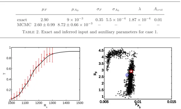
µF µA0 σF σA0 λ Acrit exact 2.90 9 × 10⁻³ 0.35 5.5 × 10⁻⁴ 1.87 × 10⁻⁴ 0.01 MCMC 2.60 ± 0.99 8.72 ± 0.66 × 10⁻³ − − − −
Table 2.Exact and inferred input and auxiliary parameters for case 1.
10000 1100 1200 1300 1400 1500 0.2 0.4 0.6 0.8 1 R x γ 0.005 0.01 0.015 1 1.5 2 2.5 3 3.5 4 4.5 µA 0 µ F 0.005 0.01 0.015 1 1.5 2 2.5 3 3.5 4 4.5 µA 0 µ F 0.005 0.01 0.015 1 1.5 2 2.5 3 3.5 4 4.5 µA 0 µ F 0.005 0.01 0.015 1 1.5 2 2.5 3 3.5 4 4.5 µA 0 µ F 0.005 0.01 0.015 1 1.5 2 2.5 3 3.5 4 4.5 µA 0 µ F 0.005 0.01 0.015 1 1.5 2 2.5 3 3.5 4 4.5 µA 0 µ F 0.005 0.01 0.015 1 1.5 2 2.5 3 3.5 4 4.5 µA 0 µ F 0.005 0.01 0.015 1 1.5 2 2.5 3 3.5 4 4.5 µA 0 µ F 0.005 0.01 0.015 1 1.5 2 2.5 3 3.5 4 4.5 µA 0 µ F 0.005 0.01 0.015 1 1.5 2 2.5 3 3.5 4 4.5 µA 0 µ F 0.005 0.01 0.015 1 1.5 2 2.5 3 3.5 4 4.5 µA 0 µ F 0.005 0.01 0.015 1 1.5 2 2.5 3 3.5 4 4.5 µA 0 µ F 0.005 0.01 0.015 1 1.5 2 2.5 3 3.5 4 4.5 µA 0 µ F 0.005 0.01 0.015 1 1.5 2 2.5 3 3.5 4 4.5 µA 0 µ F 0.005 0.01 0.015 1 1.5 2 2.5 3 3.5 4 4.5 µA 0 µ F 0.005 0.01 0.015 1 1.5 2 2.5 3 3.5 4 4.5 µA 0 µ F 0.005 0.01 0.015 1 1.5 2 2.5 3 3.5 4 4.5 µA 0 µ F 0.005 0.01 0.015 1 1.5 2 2.5 3 3.5 4 4.5 µA 0 µ F
Figure 1.Results for case 1. Left: ”measured” intermittency (symbols) including noise (error bars) and inferred mean intermittency (−) obtained from a solution of the inverse problem. Right: samples of inferred input parameters computed during the MCMC procedure (×), to-gether with the exact solution (⋆) and the mean from MCMC (square).
MCMC procedure is given in Table 2 (labelled ‘MCMC’) and visualized in Figure 1(right). A large variance can be observed for µF, while it is much smaller for µA0. This observa-tion suggests that the intermittency curve is more sensitive with respect to variaobserva-tion in amplitude A0.
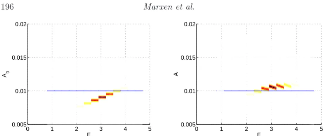
In order to illustrate the process, probability density functions of the exact solution are visualized in Figure 2. At the onset of transition (Rx = 1000), the corresponding
probability density function P DF (A0, F ) possesses appreciable values only below the
critical amplitude (Figure 2, left). In contrast, at the end of transition, almost all of these values lie above the critical amplitude, indicating that laminar-turbulent transition is complete and the flow fully turbulent (Figure 2, right).
3.2. Case 2: VKI-H3 run for a 7◦
sharp cone
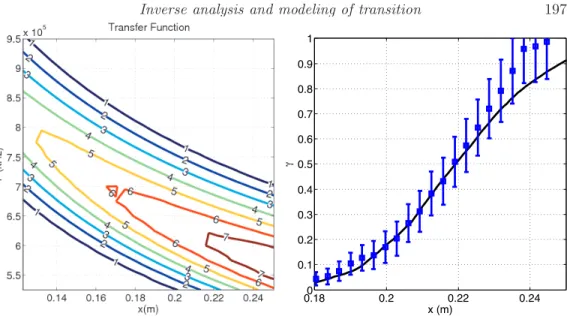
The inverse solution procedure has been applied to a test case for which measurements have been performed at the von Karman Institute for Fluid Dynamics. The transfer function N (x, F ) for this case has been computed using the LST code VESTA, which was developed at the VKI (Pinna et al. 2010; Pinna 2012). It is depicted in Figure 3 (left) for the conditions listed in Table 3. The surface N (x, F ) is discretized into 11 frequencies in the interval F ∈ [300, 800] kHz with equal spacing.
Measured heat-flux data on a 7◦
sharp cone at Mach 6 are used to compute the inter-mittency distribution, γ = γ(x), within the transition region (Eq. (2.7)). Measurement uncertainties are assumed to increase linearly from 0.1% up to 15% within the transition region as indicated by the error bars in Figure 3 (right).
The probability pT resulting from the inverse analysis with Ncrit = 5 is depicted in
0 1 2 3 4 5 0.005 0.01 0.015 0.02 F A0 0 1 2 3 4 5 0.005 0.01 0.015 0.02 F A
Figure 2. Test case 1. Left: Probability density function P DF (A0, F ) at transition onset
Rx = 1000 or x0 = 10.0. Right: Probability density function P DF (A, F ) at the end of the
transition zone Rx= 1400 or x = 19.6. The horizontal (blue) line marks the critical amplitude
Acrit. The P DF vanishes outside of the colored part.
P∞[Pa] T∞[K] ρ∞[kg/m 3
] U∞[m/s] Re∞[1/m] Twall[K]
1640.41 59.875 0.09529 931.45 2.28E+07 294.73
Table 3.Free stream conditions (subscript ∞) for case 2: VKI-H3 Mach 6 air.
and Geweke’s test (Geweke 1992) has been used to verify stochastic convergence. The parameters resulting from the inference are mean µF = 508 kHz and variance σF = 29
kHz, with a standard deviation of 10 kHz and 6 kHz, respectively. The solution matches γ derived from experimental data almost perfectly in the first part of the transition region, that is, between 0 < γ < 0.5. In the part further downstream, larger differences between experimental data and the intermittency obtained with the inverse method are visible. These differences are likely due to deficiencies of the forward model. For instance, nonlinear effects, such as the merging and growing of turbulent spots, are not captured in our LST-based model. Moreover, local LST neglects the non-parallel character of growing boundary layers. Finally, we included only two-dimensional perturbations in our analysis.
4. Conclusions
A new method has been introduced that can be applied to infer disturbance spectra at a location upstream of laminar-turbulent transition using measured intermittency curves. In the forward model, intermittency curves are computed for a given disturbance spec-trum, using linear stability theory at the core of the model. The inverse method applies a statistical analysis using the Markov chain Monte Carlo technique. The inverse method has been illustrated using a synthetic test case and has been applied to experimentally measured data. The inference procedure yields two parameters used to define a joint probability function of perturbation frequency and amplitude upstream of the transition location.
For both test cases, good agreement was found between the given noisy intermittency curve and the curve resulting from inferred spectra. This suggests that the forward model
0.180 0.2 0.22 0.24 0.1 0.2 0.3 0.4 0.5 0.6 0.7 0.8 0.9 1 x (m) γ
Figure 3.Results for case 2 with conditions specified in Table 3. Left: Contours of the N -factor. Right: Converged probability pT = γ from inverse analysis with Ncrit= 5 (line), together with
the mean intermittency inferred from experimental data (symbols) including measurement error (erro bars), which was used as an input.
is able to represent the intermittency curve sufficiently well. For the synthetic test case, it was found that the intermittency curve is more sensitive with respect to variation in the parameter governing the amplitude than with respect to the variation in the parameter related to the frequency. The relative accuracy in the inference procedure was therefore higher for the parameter related to the amplitude.
It should be noted that our method only yields frequencies equal to and lower than the one predicted by the standard eN-method, since perturbations at higher frequencies
may not induce turbulence further downstream of the onset of transition, as they will decay downstream of the location of nominal transition onset.
For the case with measured data, measured disturbance spectra are available in addi-tion to intermittency data. These data will be processed and then used in future work for a comparison with the results of our inverse analysis. We expect that the results can be improved by using a higher-fidelity forward model. Moreover, the present method relies on a number of assumptions, including the shape of the joint PDF for frequency and amplitude, as well as the kind and number of parameters that are inferred. The effect of these assumptions should carefully be assessed in the future.
REFERENCES
Geweke, J.1992 Evaluating the accuracy of sampling-based approaches to the calcu-lation of posterior moments. In Bayesian statistics, pp. 169–193. Oxford University Press, Oxford, U.K.
Hastings, W. K. 1970 Monte carlo sampling methods using markov chains and their applications. Biometrika 57 (1), 97–109.
Jacobs, R. G. & Durbin, P. A.2001 Simulations of bypass transition. J. Fluid Mech. 428, 185–212.
Unstructured Parallelized Computational Fluid Dynamics Codes. AIAA J. 47 (12), 2894–2906.
Mack, L. M. 1969 Boundary layer stability theory. Tech. Rep. JPL-900-277-REV-A; NASA-CR-131501. Jet Propulsion Laboratory, NASA.
Malik, M. R.1989 Prediction and control of transition in supersonic and hypersonic boundary layers. AIAA J. 27 (11), 1487–1493.
Malik, M. R.2003 Hypersonic flight transition data analysis using parabolized stability equations with chemistry effects. J. Spacecraft Rockets 40 (3), 332–344.
Marxen, O. & Iaccarino, G.2009 Transitional and turbulent high-speed boundary-layers on surfaces with distributed roughness. AIAA Paper 2009–171 pp. 1–13. Marxen, O., Iaccarino, G. & Shaqfeh, E. 2010 Disturbance evolution in a Mach
4.8 boundary layer with two-dimensional roughness-induced separation and shock.
J. Fluid Mech. 648, 435–469.
Mayer, C. S. J., Wernz, S. & Fasel, H. F. 2011 Numerical investigation of the nonlinear transition regime in a mach 2 boundary layer. J. Fluid Mech. 668, 113– 149.
Pinna, F.2012 Numerical study of stability of flows from low to high mach number. PhD thesis, Universit´a di Roma ‘La Sapienza’, von Karman Institute for Fluid Dynamics. Pinna, F., Bensassi, K., Rambaud, P., Chazot, O., Lani, A. & Marxen, O. 2010 Development of an integrated methodology for the post-flight analysis of the transition payload for the EXPERT mission. In Proceedings of the 2010 Summer
Program, pp. 423–432. Center for Turbulence Research, Stanford University. Pˇecnik, R., Witteveen, J. A. S. & Iaccarino, G. 2011 Uncertainty
quantifica-tion for laminar-turbulent transiquantifica-tion predicquantifica-tion in rans turbomachinery applicaquantifica-tions.
AIAA Paper 2011–0660 pp. 1–14.
Reda, D. C.2002 Review and synthesis of roughness-dominated transition correlations for reentry applications. J. Spacecraft Rockets 39 (2), 161–167.
Serino, G., Marxen, O., Pinna, F., Rambaud, P. & Magin, T. 2012a Transi-tion predicTransi-tion for oblique breakdown in supersonic boundary layers with uncertain disturbance spectrum. AIAA 2012–2973 pp. 1–11.
Serino, G., Pinna, F. & Rambaud, P.2012b Numerical computations of hypersonic boundary layer roughness induced transition on a flat plate. AIAA 2012–0568 pp. 1–16.
Tarantola, A.2005 Inverse problem theory and methods for model parameters
estima-tion. SIAM: Society for Industrial and Applied Mathematics.
Vinod, N. & Govindarajan, R. 2004 Pattern of breakdown of laminar flow into turbulent spots. Phys. Rev. Lett. 93 (11), 114501.