Social Security, Ageing and Economic Integration

Social Security, Ageing and Economic Integration

∗

Lionel Artige

CREPP

HEC - University of Li`ege

Antoine Dedry

CREPP

HEC - University of Li`ege

Pierre Pestieau

CREPP, CORE

HEC - University of Li`ege

September 25, 2012

Abstract

The purpose of this paper is to analyze the impact of economic integration when countries differ in their social security systems, more specifically in the degree of funding of their pensions, and in the flexibility in the retirement age. It then turns to the impact of ageing, namely the decline in fertility and the increase in longevity, on the welfare of these integrated countries.

Keywords: Ageing, tax competition, social security JEL Classification: H2, F42, H87

∗_{This research is financed by the Belgian Federal project BELDEBT.}

†_{Corresponding author: HEC - Universit´e de Li`ege, Economics department, Boulevard du Rectorat}

1

Introduction

It is well known that economic integration can have unpleasant implications for countries, which are relatively less indebted than others. Whether the debt we have in mind is the traditional sovereign debt or the debt that is implicit to unfunded pension schemes, allow-ing for a free capital mobility lead to an outflow from indebted countries to countries with sounder public finances. This consideration justified the Maastricht Treaty guidelines of the European Union: a deficit of less than 3% and a debt to GDP ratio not exceeding 60%. It is interesting to observe that the Maastricht Treaty was unable to touch the other less explicit forms of endebtment.

Besides endebtment, there are other national characteristics that have the same impli-cations and that have not received the same attention. One of them concerns the more or less flexibility of the retirement decision. There are a wide variety of regulations con-cerning the age of retirement across OECD countries1 and this leads to an important range in the effective age of retirement. This has some implications for saving and capital accumulation. The life cycle theory of saving is quite explicit: the later individuals retire, the less they have to save. If someone wants and is allowed to work till the end of his life he will need to save much less than someone who decides or is forced to retire at, let us say age 55, which is frequent in countries such as France or Belgium.

In this paper we are interested in the role of two features of the retirement systems in case of economic integration: whether it is funded or not and whether it implies flexible or mandatory early retirement age. Given that mandatory retirement is often associated with pay as you go (hereafter, PAYG) systems we consider what happens when two countries, one with PAYG and mandatory retirement age and one with fully funding and flexible retirement form an economic union2. We show that the question of who wins and

1_{See Fenge and Pestieau (2005).}

who loses is ambiguous, it will depend on the relative strength of those two features: the amount of unfunded pensions and the rigidity of the retirement age.

Then we turn to the question of ageing, namely the consequences of declining fertility and increasing longevity on the welfare of this economic union and of its member states. To deal with these issues, we deliberately adopt a simple two-country setting with Cobb-Douglas production and log linear utility functions. To better understand the incidence of ageing on both capital accumulation and utilities we resort to numerical examples.

2

The basic model: autarky

We use the standard overlapping generation model. An individual belonging to generation t lives two periods t and t + 1. The first one has a unitary length, while the second has a length ℓ ≤ 1, where ℓ reflects variable longevity. In the first period, the individual works and earns wt which is devoted to the first-period consumption, ct, saving st and

pension contribution τ . In the second period he works an amount of time zt+1 ≤ ℓ ≤ 1

and earns zt+1wt+1. This earning plus the proceeds of saving Rt+1st and the PAYG

pension p finances second period consumption dt+1. Working zt+1 implies a monetary

disutility v (zt+1, ℓ) where ∂v_∂ℓ < 0 reflects the idea that an increase in longevity fosters

later retirement.

Denoting by u (·) the utility function, the problem of an individual of generation t is:

max U = u (wt− τ − st) + βℓu ( wt+1zt+1+ Rt+1st+ p− v (zt+1, ℓ) ℓ ) (1)

where p = τ (1+n) and β is the time discount factor. (1+n) is the gross rate of population growth and also the number of children per individual.

The FOC’s are simply: v_z′ t+1(zt+1, ℓ) = wt+1 −u′_(c t) + βRt+1u′ ( ˜ dt+1 ) = 0 where ˜dt+1 = dt+1−v(z_ℓ t+1,ℓ).

We will use simple forms for u (·) and v(·): u (x) = ln x and v (x) = x2_{/2γℓ where}

γ ∈]0, 1] is a preference parameter. One clearly sees that the disutility of working longer is mitigated by an increase in longevity. We can now write the problem of the individual as: ln (wt− τ − st) + βℓ ln  wt+1zt+1+ Rt+1st− z2 t+1 2γℓ + p ℓ   , (2)

where p = τ (1 + n). The FOC with respect to zt+1 and st yield

zt+1 = γℓwt+1 (3) st = βℓ 1 + βℓwt− γℓw2 t+1 2Rt+1(1 + βℓ) − τ ( βℓ 1 + βℓ+ 1 + n (1 + βℓ) Rt+1 ) (4)

We now turn to the production side. We use a Cobb-Douglas production function

Yt = F (KtNt) = AKtαNt1−α (5)

where the labor force is Nt = Lt+ Lt−1zt = Lt−1(1 + n + zt). We distinguish Nt the labor

force and Lt the size of generation t. We assume that

Total population at time t is

Lt+ ℓLt−1 = Lt−1(1 + ℓ + n) .

Denoting Kt/Nt ≡ kt and Yt/Nt ≡ yt, we obtain the income per capita

yt= f (kt) = Aktα

and the factor prices

Rt = f′(kt) = Aαktα−1

wt = f (kt)− f′(kt)kt= (1− α) Akαt

Resource constraint at time t implies

f (kt) = ct+

ℓdt

1 + n + (1 + n) kt+1

while the equilibrium conditions in the labor and capital markets are respectively

Nt = Lt−1(1 + n + zt)

Kt+1 = Ltst

We can now write the dynamic equation with perfect foresight

i.e., (1 + n) kt+1+ γℓA (1− α) kα+1t+1 = βℓ 1 + βℓA(1− α)k α t − γℓk_t+11+αA2(1− α)2 2 (1 + βℓ) Aα −τ ( βℓ 1 + βℓ + (1 + n) k_t+11−α Aα (1 + βℓ) ) or 2Aα(1 + ℓβ)(1 + n)kt+1− 2ℓA2αβ(1− α)ktα+ 2τ (1 + n)kt+11−α+ (7) 2A2_{ℓγα(1 + ℓβ)(1− α)k}(1+α) t+1 + γℓA2(1− α)2k α+1 t+1 + 2Aℓατ β = 0

Differentiating totally Equation (7) taken in the steady state and assuming both stability and unicity of k∗, namely 0 < dkt+1

dkt

< 1, we show in the appendix:

dk∗ dτ∗ < 0 , dk∗ dγ < 0 , dk∗ dn < 0.

These three inequalities are standard. It is indeed well-known that a PAYG pension (τ ) depresses capital accumulation, that working longer (γ) has a negative impact on saving and that a lower fertility rate (n) increases the steady-state capital stock. However, the effect of an increase in longevity on capital accumulation is ambiguous:

dk∗

dℓ =−2Aℓ

−2_{α(1 + n)k}∗_{− 2τℓ}−2_{(1 + n)k}∗_{+ 2A}2_{αβγ(1− α)k}∗1+α_{≷ 0 (8)}

This inequality is more surprising and its ambiguity depends on the presence of a flexible age of retirement along with a PAYG system. Without pension and flexible retirement, increasing longevity unambiguously fosters capital accumulation.

It is important to note at this point that some of these results, particularly the unam-biguous comparative statics, comes from our particular specification of preferences and

technology.

3

Economic union

Let us assume that we have two countries that are identical in all respects but in the values of their preference for retirement (γ) and the degree of prefunding of their pension system. We denote these countries A and B. Country A has a PAYG pension system with mandatory retirement at the end of the first period. Country B has a fully funded pension system with flexible retirement age. Assuming that γA= 0 is a statement on the

nature of preferences. However this has the same formal implications as having any value of γ but constraining z to be equal to 0. Henceforth in this paper to mean that early retirement is mandatory, that is that people must retire at the end of the first period regardless of longevity, we posit that γ is nil. Therefore, the consumer’s preferences in country A and B are as follows:

UA = ln(wA,t− τA− sA,t) + βℓ ln ( RA,t+1sA,t+ pA ℓ ) (9) UB = ln(wB,t− sB,t) + βℓ ln ( wB,t+1zB,t+1+ RB,t+1sB,t− vB(zB,t+1, ℓ) ℓ ) (10)

As long as the two countries are autarkic, their GDP and welfare will depend on their saving. The optimal saving for country A and country B are:

sA,t = βℓ 1 + βℓwA,t− τA ( βℓ 1 + βℓ + 1 + n (1 + βℓ)RA,t+1 ) (11) sB,t = βℓ 1 + βℓwB,t− γBℓwB,t+12 2RB,t+1(1 + βℓ) (12)

for any t

RA,t= RB,t

or

kA,t= kB,t = kt

When capital markets are integrated, the difference in saving between both countries is

sB,t− sA,t= τA βℓ 1 + βℓ + τA (1 + n) Aα (1 + βℓ)k 1−α A,t+1− γBℓA2(1− α)2 2Aα (1 + βℓ) k 1+α B,t+1 (13)

Clearly, if τAis relatively higher than γB, one expects to have a higher steady-state capital

stock and a higher GDP in B than in A. The equilibrium in the integrated capital market is given by Lt(sAt + sBt) = KA,t+1+ KB,t+1 (14) or sA,t+ sB,t = 2kt+1(1 + n) + kt+1zB,t+1 (15) 2 (1 + n) kt+1+ γBℓA (1− α) kt+11+α = 2Aβℓ 1 + βℓ(1− α) k α t − γBℓA2(1− α)2 2Aα (1 + βℓ) k 1+α t+1 − τAβℓ 1 + βℓ− τA(1 + n) Aα(1 + βℓ)k 1−α t+1. (16)

From Equation (16), one obtains kt+1and then one is able to calculate the flow of capital

by: MAB = (1 + n)kA,t+1− sA,t (17) = (1 + n) kt+1− Aβℓ 1 + βℓ(1− α) k α t + τAβℓ 1 + βℓ+ τA(1 + n) Aα (1 + βℓ)k 1−α t+1 (18)

At the world level, the flows of capital between two countries must necessarily offset each other:

MAB+ MBA= 0 (19)

4

Numerical examples.

To better grasp the sensitivity of the solutions to changes in policy parameters τ and γ as well as to changes in demographic parameters, fertility n and longevity ℓ, we resort to numerical simulations. In these simulations, we use the same specification as above with: yt = Aktα where A = 50 and α = 1/3. As to preferences, β = 1. The other parameter

values are given in the tables.

We see that in autarky the steady state capital accumulation decreases with fertility, longevity, PAYG pensions and retirement flexibility. The results were already obtained analytically except for longevity, which has an ambiguous effect for a large γ.

We then turn to an economic union with perfect capital mobility between two countries, one with a PAYG and mandatory early retirement and one with flexible retirement but funded pensions. Not surprisingly the overall capital stock will be depressed by the presence of either PAYG or flexible retirement. The direction of capital flow depends on the relative importance of the PAYG scheme relative to the flexibility in the age of retirement.

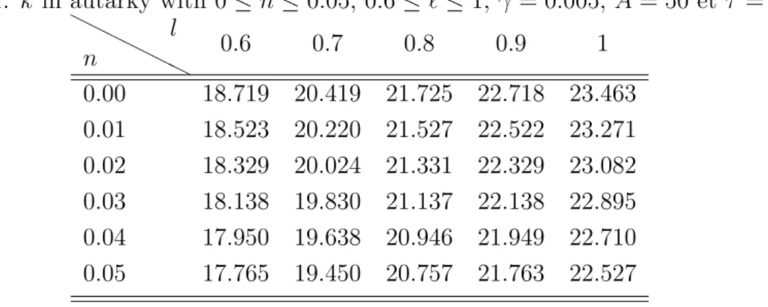
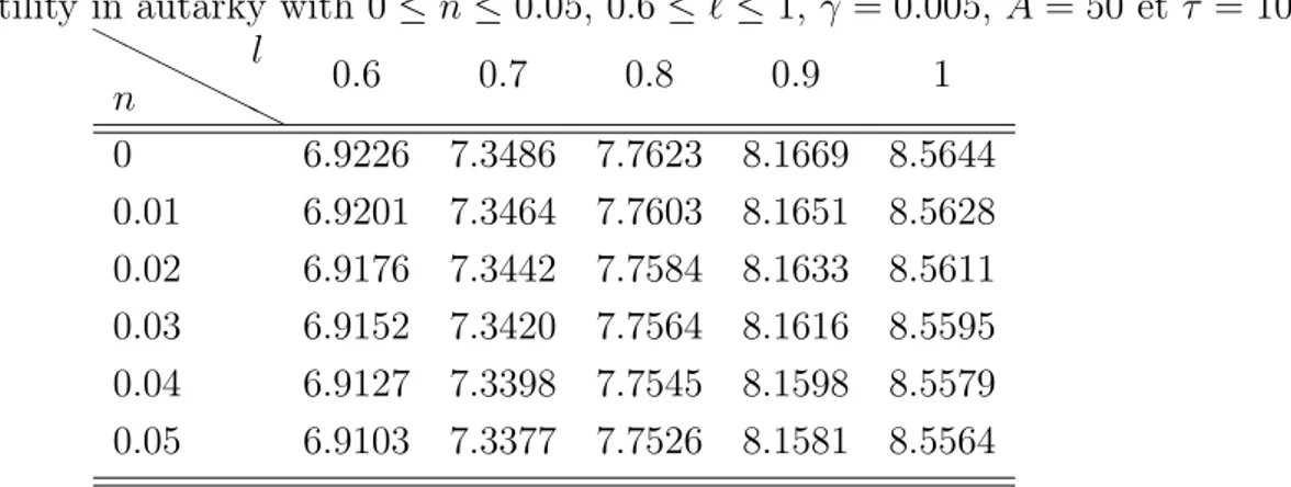
Our primary interest is the welfare of individuals. The main results are that a PAYG scheme depresses welfare in the steady state and flexible retirement has an ambiguous effect: positive impact because for a given capital stock it provides more resources to the individual and negative because it induces less saving. Table 1 indicates that, in autarky, the capital stock per capita at the steady state decreases with n and increases with ℓ. The first result was expected; not the second. Table 2 gives the level of welfare at the steady state for various values of n and ℓ. The results are the same as previously: utility decreases with n and increases with ℓ. Tables 3 and 4 deal with the case of an economic union with country A having a PAYG social security with mandatory early age of retirement and country B having a fully funded pension system with late flexible retirement. Here again k increases with ℓ and decreases with n. We have the same pattern for the utilities in the two countries except for certain values of ℓ approaching 1 when the parameter values of A and γ are high. In these cases, we have that ∂UA

∂n > 0. In other words, the country with

PAYG and mandatory retirement age sees its welfare increases when n increases. Table 1: k in autarky with 0≤ n ≤ 0.05, 0.6 ≤ ℓ ≤ 1, γ = 0.005, A = 50 et τ = 10

HH HH_HH n l 0.6 0.7 0.8 0.9 1 0.00 18.719 20.419 21.725 22.718 23.463 0.01 18.523 20.220 21.527 22.522 23.271 0.02 18.329 20.024 21.331 22.329 23.082 0.03 18.138 19.830 21.137 22.138 22.895 0.04 17.950 19.638 20.946 21.949 22.710 0.05 17.765 19.450 20.757 21.763 22.527

Table 2: Utility in autarky with 0≤ n ≤ 0.05, 0.6 ≤ ℓ ≤ 1, γ = 0.005, A = 50 et τ = 10 HH HH_HH n l 0.6 0.7 0.8 0.9 1 0 6.9226 7.3486 7.7623 8.1669 8.5644 0.01 6.9201 7.3464 7.7603 8.1651 8.5628 0.02 6.9176 7.3442 7.7584 8.1633 8.5611 0.03 6.9152 7.3420 7.7564 8.1616 8.5595 0.04 6.9127 7.3398 7.7545 8.1598 8.5579 0.05 6.9103 7.3377 7.7526 8.1581 8.5564

Table 3: k global with 0≤ n ≤ 0.05, 0.6 ≤ ℓ ≤ 1, γB = 0.005, A = 50 et τA= 10

HH HH_HH n l 0.6 0.7 0.8 0.9 1 0.00 27.393 30.263 32.603 34.503 36.036 0.01 27.076 29.929 32.261 34.155 35.686 0.02 26.764 29.602 31.923 33.813 35.342 0.03 26.458 29.279 31.591 33.475 35.003 0.04 26.157 28.962 31.264 33.143 34.669 0.05 25.862 28.650 30.942 32.816 34.340 τB = 0, γA= 0

T able 4: Utilit y in A and B in economic union with 0 ≤ n ≤ 0 .05, 0 .6 ≤ ℓ ≤ 1, τA = 10, A = 50 et γB = 0 .005 H H H H H H n l 0.6 0.7 0.8 0.9 1 0 6.9138; 7.1143 7.2998; 7.5406 7.6701; 7.9575 8.0282; 8.3673 8.3765 ; 8.7716 0.01 6.9122; 7.1113 7.2986; 7.5377 7.6694; 7.9546 8.0280; 8.3644 8.3767 ; 8.7686 0.02 6.9105; 7.1084 7.2975; 7.5348 7.6688; 7.9517 8.0278; 8.3615 8.3769 ; 8.7657 0.03 6.9089; 7.1055 7.2964; 7.5320 7.6682; 7.9489 8.0276; 8.3586 8.3771 ; 8.7628 0.04 6.9073; 7.1026 7.2953; 7.5292 7.6675; 7.9461 8.0274; 8.3558 8.3773 ; 8.7600 0.05 6.9056; 7.0998 7.2942; 7.5264 7.6669; 7.9434 8.0272; 8.3531 8.3775 ; 8.7571 τB = 0 ,γ A = 0

5

Conclusion

In this paper we have tried to evaluate the economic implications of ageing on the welfare of economic unions whose member states have different social security regimes. We have chosen a setting in which some countries have a PAYG system along with mandatory early age of retirement; as to the other members of the union, their social security is fully funded and retirement totally flexible. The interesting finding is that the latter can end up with less capital accumulation than the former. We have studied the effect of ageing on the equilibrium values of this economic union. We distinguish two factors of ageing: increasing longevity and declining fertility rate. Both factors have a stimulating effect on capital accumulation. It should be noted however that these findings are only relevant for the steady-state. Results are likely to be different in the short run dynamics. Among possible extensions, we would like to adopt more general utility and production functions and to increase the types of countries involved in the tax competition game.

References

[1] Fenge, R. and P. Pestieau (2005), Social security and Retirement, MIT Press.

[2] OECD (2011), Pensions at a Glance 2011: Retirement-income Systems in OECD and G20 Countries, OECD Publishing.

[3] EC (2008), The 2009 Ageing Report: Underlying Assumptions and Projection Method-ologies, European commission.

6

Appendix

Dividing by ℓ the accumulation rule of capital (Equation (7)), we obtain

G = 2Aα(1 + ℓβ)(1 + n)kt+1− 2ℓA2αβ(1− α)ktα+ 2τ (1 + n)k

1−α

t+1 + (20)

2A2ℓγα(1 + ℓβ)(1− α)k_t+1(1+α)+ γℓA2(1− α)2kα+1_t+1 + 2Aℓατ β = 0

we differentiate (20) with respect to ℓ, n, τ , γ, kt+1 and kt are

∂G ∂ℓ =−2Aℓ −2_{α(1 + n)k} t+1− 2τℓ−2(1 + n)k1−α+ 2A2αβγ(1− α)kt+11+α (21) ∂G ∂n = 2Aα(1 + ℓβ)kt+1+ 2τ k 1−α t+1 > 0 (22) ∂G ∂τ = 2Aℓαβ + (1 + n)k 1−α t+1 > 0 (23) ∂G ∂γ = 2A 2 ℓα(1 + ℓβ)(1− α)k1+α_t+1 + ℓA2(1− α)2k1+α_t+1 > 0 (24) ∂G ∂kt+1 = 2Aα(1 + n)(1 + ℓβ) + 2A2ℓγα(1 + ℓβ)(1− α)k_t+1α + (25) A2ℓγ(1− α)2k_t+1α + 2τ (1− α)(1 + n)k_t+1−α > 0 ∂G ∂kt =−2α2A2ℓβ(1− α)k_tα−1 < 0 (26)

Stability and unicity imply that:

0 <− ∂G ∂kt ∂G ∂kt+1 < 1 Hence : ∂G ∂kt+1 +∂G ∂kt > 0

and in the steady state where kt = kt+1 = k :

∂G ∂k > 0

From the above expressions, we clearly have the following properties at the steady state:

dk dn < 0 dk dγ < 0 dk dτ < 0 dk dℓ ≷ 0