Bénard instabilities in a binary-liquid layer evaporating into an inert gas: stability of quasi-stationary and time-dependent reference profiles

(will be inserted by the editor)

B´

enard instabilities in a binary-liquid layer

evaporating into an inert gas: stability of

quasi-stationary and time-dependent reference

profiles

Universit´e de Li`ege, Institut de Physique B5a, All´ee du 6 Aoˆut 17, B-4000 Li`ege, Belgium

2

Universit´e Libre de Bruxelles, TIPs - Fluid Physics, CP165/67, Avenue F.D. Roosevelt, 50, B-1050 Bruxelles, Belgium

Abstract. This study treats an evaporating horizontal binary-liquid layer in con-tact with the air with an imposed transfer distance. The liquid is an aqueous solution of ethanol (10 % wt). Due to evaporation, the ethanol mass fraction can change and a cooling occurs at the liquid-gas interface. This can trigger solutal and thermal Rayleigh-B´enard-Marangoni instabilities in the system, the modes of which corresponding to an undeformable interface form the subject of the present work. The decrease of the liquid-layer thickness is assumed to be slow on the diffusive time scales (stationarity). First we analyse the stability of quasi-stationary reference profiles for a model case within which the mass fraction of ethanol is assumed to be fixed at the bottom of the liquid. Then this consideration is generalized by letting the diffusive reference profile for the mass fraction in the liquid be transient (starting from a uniform state), while following the frozen-time approach for perturbations. The critical liquid thickness below which the system is stable at all times quite expectedly corresponds to the one obtained for the quasi-stationary profile. As a next step, a more realistic, zero-flux condition is used at the bottom in lieu of the fixed-concentration one. The critical thickness is found not to change much between these two cases. At larger thicknesses, the critical time at which the instability first appears proves, as can be expected, to be independent of the type of the concentration condition at the bottom. It is shown that solvent (water) evaporation plays a stabilizing role as compared to the case of a non-volatile solvent. At last, an effective approximate Pearson-like model is invoked making use in particular of the fact that the solutal Marangoni is by far the strongest as an instability mechanism here.

1 Introduction

Convective instabilities of horizontal liquid layers are associated with destabilizing vertical tem-perature or concentration gradients imposed on the system [1],[2],[3]. One speaks of a Rayleigh-B´enard or a Marangoni-Rayleigh-B´enard instability depending on whether it is due to buoyancy or surface tension variations. Depending on whether this stems from either the concentration dependence of the density and the surface tension or from their temperature dependence, we speak of so-lutal _{Rayleigh-Marangoni-B´enard instabilities or of thermal ones. An additional twist here is} that the solutal mechanisms can also act even when it is only temperature gradients that are

a

imposed from outside, this being due to the Soret effect.

For an evaporating horizontal liquid layer, vertical temperature gradients result already from an evaporation-induced cooling of the interface, be it even in the absence of externally imposed temperature differences. In the case of binary mixtures, evaporation-induced concentration gradients occur as well. This means that evaporation can indirectly destabilize the liquid layer through the thermal and solutal Rayleigh-Marangoni mechanisms. While the evaporation of one-component liquids has been studied rather thoroughly in the literature (e.g. [4], [5] [6],[7], to mention a few), fewer studies exist in what the evaporation of two-component systems into an inert gas is concerned: a theoretical study in a horizontal liquid layer involving the thermal and solutal Rayleigh and Marangoni effects and also taking into account the Soret effect [8], a theoretical study for a droplet with thermal and solutal Marangoni effects [9], a scaling analysis [10], a number of experiments reported e.g. in [11],[12], and the present paper is yet another contribution along this line.

It should be noted that the evaporation process makes the thickness of the liquid layer vary with time. The majority of works in the literature rely upon the quasi-stationary assumption in the sense that this variation is slow as compared to the diffusive time scales in the system, and such will also be the case in the present paper. This means that the thickness remains effectively constant on the relevant time scales of the problem. On the other hand, within this framework, one can speak of a quasi-stationarity in another sense: the reference profiles themselves may be either quasi-stationary (as e.g. in [8], [9]) or transient (as e.g. in [12]). In the present paper, the accent is primarily on the latter situation, even though we make a connection with the previous, quasi-stationary study [8], and the frozen-time approach is used for the perturbations.

Thus, in the previous work [8], we have analyzed the stability of a quasi-stationary reference profile in a binary-liquid layer, the quasi-stationarity being made possible thanks to a (some-what artificial) assumption of a constant mass fraction imposed at the bottom. This system turned out to be highly unstable in the water-ethanol case, with critical liquid thicknesses typ-ically about 10 nm to 1 µm, increasing with the transfer distance in the gas. Comparing the Marangoni and Rayleigh, thermal and solutal effects with one another, we have shown that the Marangoni effect is much more important than the Rayleigh effect (which is not surpris-ing in view of such small critical liquid thicknesses) and that the solutal effect is also by far more important than the thermal effect considering an initial solute (ethanol) mass fraction of 0.1. When considering an initial solute mass fraction of 0.001, the thermal effect appeared to become more important, even though the solutal one still remained the strongest. It was thus concluded that the instability mechanism is primarily of the solutal Marangoni type. Given the extremely small critical liquid layer thicknesses obtained in our analysis, we deduce that an initially well mixed binary liquid with a realistic thickness of, say, 1 mm should become unstable very shortly after its exposure to air, much before the transient diffusional boundary layers developing from the free surface have reached the bottom of the liquid. Thus, studying the instability with time-dependent reference profiles is in principle of sufficient interest. In this paper, in a more general model than in [8], we consider an actual time evolution of the concentration profile in the liquid and at the same time include a more realistic concentra-tion condiconcentra-tion at the bottom rendering such a transient consideraconcentra-tion indispensable. Yet the quasi-stationary assumption is retained in the gas phase as well as for the temperature. This represents a reasonable step forward indeed, given that the time scale for ethanol diffusion in the liquid is typically much greater than the thermal diffusion time scale and the corresponding time scales in the gas phase (Dl<< κl, κg, Dg) provided that the gas layer thickness (associated

with a transfer distance here, cf. [8]) is not too big. Dl and Dg are the diffusion coefficients,

while κland κgrepresent the thermal diffusivity in respectively the liquid and gas phases. The

subscripts l and g hereafter refer to the liquid and the gas. The essentials of the formulation are presented in more detail in [8], the main difference here being, as already mentioned, a transient mass fraction reference profile in the liquid phase and two variants of the concentra-tion condiconcentra-tion at the bottom of the liquid layer. First, in order to draw a parallel with [8], we assume thereat a fixed mass fraction. Then, the model is rendered more realistic by assuming a zero mass flux instead. As in [8], we consider a dilute solution (of ethanol in water) of which the solute (ethanol) is volatile in all cases, whereas two kinds of treatment are used in what

the volatility of the solvent (water) is concerned: it is either neglected altogether or taken into consideration. The aim of the paper is to study the instability threshold in terms of critical liquid thicknesses (below which no instability occurs at any time) and critical times (at which the instability first occurs in accordance with the frozen-time approach for thicknesses above the critical). In doing so, the degree of mutual importance of different instability mechanisms is also assessed along the lines of [8].

2 Model description

As already mentioned, the system of interest in this paper is quite similar to the one studied in [8]. So here we recall only the main assumptions and stress the differences.

A sketch of the system is presented in Fig. 1. The physical system is a horizontal binary-liquid (water-ethanol) layer of thickness dl evaporating into an inert gas from a free flat interface on

which a local phase equilibrium is assumed. The gas layer, of thickness dg, consists of a mixture

of an inert gas and the vapors of the solute (ethanol) and the solvent (water). At a distance dg

above the interface (the transfer distance in the gas) a fixed vapor concentration is assumed, which in the present paper will be taken equal to zero, as well as a fixed temperature and pressure of the environment. Air absorption in the liquid is neglected.

Fig. 1. Sketch of the system

The equations in the bulk of the liquid and gas phases and the boundary conditions except for one (see below) are the same as presented in [8]. In particular, the Boussinesq approximation is used, where the density in the liquid and gas phases linearly depends on the temperature and concentration in the buoyancy terms, while all bulk fluid properties are considered as constant at other places. The boundary conditions at the top of the gas phase are a constant normal stress, a zero shear stress, a constant fixed ambient temperature Tb (the same as at the

bottom of the liquid layer) and a fixed (here zero) mass fraction of the vapor. At the interface the following conditions are involved: the tangential stress balance including the thermal and solutal Marangoni stresses, the no-slip condition, the temperature continuity, the heat flux balance including the heat of evaporation, the mass flux conservation (total and for each of the species), the local equilibrium (Henry’s law for the solute and Raoult’s law for the solvent). At the bottom of the liquid layer we consider a constant temperature Tb (the same as at the top of

the gas layer), the no-slip condition, a zero normal velocity. As for the concentration condition at the bottom, in [8] we used

cl= cb, (1)

where cl is the solute (ethanol) mass fraction field in the liquid layer and cb is a fixed value,

whereas the present paper deals for the most part with a more realistic, zero-flux condition instead:

∂cl

∂z + ψS ∂Tl

where ψS = θD_DT ,l_l cb(1 − cb) (Soret separation parameter), with DT ,land Dlbeing respectively

the thermal diffusion coefficient and the diffusion coefficient. Tl is the liquid temperature field

non-dimensionalized by substracting Tb and dividing by a temperature scale θ. In the case of

Eq. (2), cb will refer to the initial mass fraction in the liquid layer, and thus note that Eq. (1)

will also formally serve as the initial condition in all transient-profile calculations here. For more details and a full mathematical formulation of the problem, see [8], where the values of physico-chemical properties of the water-ethanol system can also be consulted. We use Tb = 300K for

the ambient temperature and cb= 0.1 here throughout.

3 Reference profiles

In order to perform a linear stability analysis, it is necessary to know the (horizontally uniform) reference profiles of the mass fraction and the temperature in both the liquid and the gas phases. In the gas phase, as well as for the temperature in the liquid phase, these are assumed to be quasi-stationary, as already described in section 1. Thus, they are of the same form as in [8]. On the other hand, the reference mass fraction profile in the liquid, cl,ref, is transient and satisfies

∂cl,ref

∂t =

∂2

cl,ref

∂z2 , (3)

where t and z are the dimensionless time and vertical coordinate with the scales d2

l/Dl and

dl respectively (note that the time scale used in [8] was different by a factor of Lel = D_κll).

For the boundary condition at the bottom (z = 0), we use either (1) or (2) in terms of cl ≡

cl,ref, whereas (1) is taken as the initial condition in either case. The (non-linear) boundary

conditions at the interface (z = 1) are the same as in [8]. The problem for the reference profiles is numerically discretisized, using a semi-implicit finite difference method scheme. The values at the interface are found by means of a Newton-Raphson routine. In Fig. 2, examples of the reference solution are presented for the mass fraction for the case H = 11, where H ≡ (dl+ dg)/dl, considering either the fixed-concentration or zero-flux conditions at the bottom of

the liquid.

Fig. 2.Mass fraction profiles in the liquid as a function of the z-coordinate for H = 11 and cb= 0.1,

considering the fixed-concentration (left) and zero-flux (right) conditions at the bottom, and corre-sponding to t=0.00315, 0.0126, 0.0315, 0.126, 0.315 and 1.26. The dashed line represents the stationary mass fraction profile that is eventually attained in the first case

Fig. 2 shows that for small values of t, when the developing concentration boundary layer has not yet reached the bottom, the reference profiles naturally do not depend on the bottom condition, which is obviously not the case for bigger t. A stability analysis for these reference profiles is carried out in the following sections.

4 Principles of the stability analysis

With the exception of the bottom boundary condition for the mass fraction, for which we can use Eq. (2) instead of Eq. (1), the form of the problem for perturbations is here the same as in [8], even though the reference profiles themselves are of course different. Using the frozen-time approach and the normal-mode representation, we obtain for each time t an eigenvalue problem for the complex growth rates σ as function of the wavenumber k and other parameters of the problem. This eigenvalue problem is solved by using the Tau-Chebyshev decomposition method (a classical method that can be consulted in, for instance, [13]). The marginal condition is then determined by σ = 0 (here it turns out that the eigenvalues σ are all real and thus the instability monotonic). Chosen the liquids and the ambient conditions, the main control parameters we are left with are dl and dg (or, equivalently, dl and H). Other key parameters are t and k. In

the present paper, we limit ourselves to a parametric study at fixed values of H. We expect to obtain a critical value of dlbelow which all σ < 0 at all times t > 0 and for all k. On the other

hand, for dlgreater than this critical value, we expect to calculate the instants of t at which the

system passes through the marginal condition (σ = 0) at a certain k, that is the critical times. We note that should the system be stable just at a finite time interval (as can be expected here for the case with a zero mass flux at the bottom), there will formally be two critical times, one corresponding to the onset of the instability, the other to its extinction, of which it is the first one that is primarily of interest.

5 Results

5.1 Model validation for a fixed concentration at the bottom

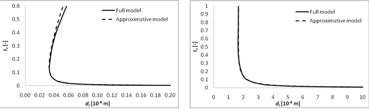
In this subsection, the stability-analysis results corresponding to the fixed-concentration con-dition at the bottom of the liquid are presented and compared with [8]. Here, as well as in the following subsection, it is assumed that it is only the solute (ethanol) that evaporates from the binary mixture. The critical time as a function of dlis represented in Fig. 3 (left) for H = 11.

It can be clearly seen that the critical value of dl corresponds to t → ∞, and thus to the

quasi-stationary reference profile the instability of which was studied in [8]. Thus, among the transient reference profiles shown in Fig. 2 (left), it is the final, quasi-stationary profile that is the most unstable. In this previous work [8], limited to the quasi-stationary case, it has been pointed out that the solutal Marangoni mechanism is the most important one at the onset of instability. At the end of this section, it will be checked whether this is still the case for the transient profiles studied in this work.

Fig. 3.Dimensionless critical time as a function of the liquid thickness comparing the quasi-stationary model [8] to the model with transient liquid mass fraction reference profiles in the case of a fixed concentration at the bottom (left) and comparing the transient-profile results in the cases of fixed-concentration and zero-flux conditions at the bottom (right), both for H = 11 and cb= 0.1

5.2 Zero flux versus fixed concentration at the bottom

The present subsection concerns the instability thresholds of the system with transient reference profiles for the liquid mass fraction. The two bottom boundary conditions for the mass fraction are compared: the fixed-concentration condition (1) and the zero-flux condition (2). The results are represented in Fig. 3 (right) for H = 11. A noteworthy feature is that the values for the critical time for the two models approach one another for large liquid thicknesses, for which the dimensionless critical time tc→ 0. This means that in the beginning of the evolution, regardless

of the bottom condition for the mass fraction, the instability threshold is the same. This can be understood by mentioning that in the beginning, the developing diffusive boundary layer of the reference profile has not yet reached the bottom of the liquid layer. Therefore, the instability threshold in terms of tc is not affected by the boundary condition for the mass fraction at the

bottom. As soon as it has reached the bottom, however, this is no longer the case. For the fixed-concentration case, the ethanol keeps being provided from the bottom, so that a quasi-stationary state is reached (cf. Fig. 2 (left)). That is why, for dl greater than its critical value

corresponding to the quasi-stationary reference profile, the system remains unstable for t → ∞ (while neglecting the evaporation-caused decrease in the liquid layer thickness on the relevant time scales, as done in the present model). In the contrary, for the zero-flux case, ethanol is not provided from the bottom, but is rather getting depleted. In this case, the system is more stable: on the one hand, the critical value of dl(below which no instability occurs) is about 15% bigger

than in the previous case (even though here one cannot help but appreciate a good quality of estimation yielded by that simpler, quasi-stationary consideration with a fixed-concentration condition at the bottom), and on the other hand, the tcversus dlcurve manifests a turning point

at the times at which the transient reference profile can be said to have reached the bottom (cf. Fig 2 (right)) meaning that the reference profile gradients can only decrease henceforth. Now the upper branch of this curve can be interpreted as the thresholds above which the system would regain stability if the reference profiles had not been perturbed by the instability that has set in at shorter times.

5.3 Effect of considering water evaporation

Water evaporation was neglected in the previous two subsections. If now it is accounted for assuming zero humidity at the top boundary of the gas layer (cf. [8]), the results change as displayed in Fig. 4 (left), where the case with a zero-flux condition at the bottom is taken up. It shows that water evaporation is a stabilizing effect, as manifested both by higher values of the critical time for instability to start for a given liquid thickness and by a larger value of the critical dl. This actually reveals a strong solutal Marangoni nature of the instability (as

will be shown later on in subsection 5.5). Indeed, while the thermal Marangoni and Rayleigh effects, augmented by water evaporation, nonetheless still remain a small contribution, the concentration inhomogeneities in the liquid get smoothened if water evaporates together with ethanol, hence a more stable system. The stabilizing effect is here remarkably of the same order of magnitude as established in [8] in the case of a fixed concentration at the bottom and a quasi-stationary reference profile.

5.4 Critical wavenumbers

Fig. 4 (right) shows the dimensionless (scale d−1

l ) critical wavenumbers kcversus the

dimension-less time for all the cases previously discussed in the present section. We observe in particular that higher values of kc (smaller sized instability patterns relative to the liquid layer thickness)

take place at small times.

5.5 The most important instability mechanism

As already mentioned, there are several mechanisms that can contribute to the numerically observed monotonic instability: solutal and thermal Marangoni and Rayleigh effects together

Fig. 4. Dimensionless critical time as a function of the liquid thickness with and without water evap-oration (left) and dimensionless critical wavenumbers as a function of the dimensionless time (right), both for H = 11 and cb= 0.1

with the corresponding Soret contributions. Interestingly enough, the ”sign” of all these effects in the liquid layer in our water-ethanol setup makes them all destabilizing and thus contributing to the monotonic instability [8]. Yet it was the solutal Marangoni one that has been found to be by far predominant in what the instability threshold is concerned in the case of a quasi-stationary reference profile with a fixed concentration at the bottom [8]. Nothing changes in this regard in the case of transient reference profiles and a zero-flux condition considered in the present paper, and the predominance of the solutal Marangoni effect is clearly illustrated in Fig. 5. All the dimensionless numbers involved are defined in a standard way [8], but here we have defined them at each t using the actual instantaneous concentration or temperature difference between the interface and the bottom within the transient reference profile.

Fig. 5.Relative importance of the solutal, thermal and Soret Marangoni and Rayleigh contributions (respectively the numbers M s∗_{, M a}∗_{, M}∗

ψ, Rs∗, Ra∗ and R∗ψ) along the marginal states in the case

of zero flux at the bottom and without (left) or with (right) water evaporation, all for H = 11 and c_{b= 0.1}

As one can observe from Fig. 5, accounting for water evaporation quite expectedly increases the role of the thermal effects, yet this is not enough to overtake the solutal Marangoni one. Note also that the very model used here (transient profiles for the concentration and yet quasi-stationary ones for the temperature) tends to artificially exaggerate the role of the thermal effects at sufficiently small times (t → 0), for in this way the temperature profile reaches the bottom formally instantaneously while the developing concentration one has not yet penetrated far below the interface.

6 Approximate model

In the present section, the approximate model developed in [8] is applied to situations involving transient profiles of interest here. Only the physical phenomena conjectured to be important enough (from the viewpoint of the instability threshold) are kept therein, and one way to justify the conjectures made is a good a posteriori agreement with the results of a full model. Apart from the physical insight, the approximate approach leads to a much less involved formulation tractable either analytically or with a lesser amount of numerical work.

First of all, given that the predominant instability mechanism is the solutal Marangoni one (cf. subsection 5.5), we neglect the Rayleigh, Soret and thermal Marangoni effects altogether. Sec-ond, as shown in [8], the typical temperature differences in our water-ethanol system prove to be small enough as to neglect the temperature dependences of the Henry coefficient of ethanol and of the saturation pressure of water. In this case, we end up with a totally isothermal for-mulation (the problem for the concentration field is decoupled from the thermal one). Third, convective effects in the gas phase are neglected for both the reference profiles and the pertur-bations, leading to purely conductive concentration fields therein, which is justified on account of small vapor concentrations in the present setup [8]; besides the dynamic viscosity of the gas is neglected versus that in the liquid. This permits an effective reduction of the two-layer problem to a one-layer formulation. In particular, the interface boundary conditions for the concentration field in the liquid can be written in a self-contained form, without invoking the corresponding variables in the gas. Thus, for the reference profile we have

∂cl,ref ∂z = ρD H − 1 cl,ref(1 − cl,ref) 1 + cl,ref(δM − 1) Ke− δDpsat1 ´ δMpdt (4) at the interface (z = 1). Here, ρ and D are respectively the gas-to-liquid ratios of the densities and diffusion coefficients. Ke, psat1 and pdt stand for respectively the Henry coefficient (of

ethanol), the saturation vapor pressure (of water) and the atmopheric pressure. δM and ´δM

represent the molar mass ratios of respectively water to ethanol and air to water, while δD

stands for the vapor diffusion coefficient ratio of water to ethanol. Eq. (4) follows from equation (98) with (100) and (101) in [8] while neglecting the Soret effect and choosing a zero humidity, both in water and in ethanol, at the top of the gas layer (ct1 = ct2 = 0). The case with

no water evaporation formally corresponds to psat1 ≡ 0. The problem for cl,ref(t, z) is thus

given by Eq. (3) with the interface boundary condition (4), the bottom (z = 0) boundary condition cl,ref = cb(fixed concentration) or ∂cl,ref/∂z = 0 (zero flux) and the initial condition

cl,ref = cb (cf. (1) and (2) while neglecting the Soret effect). Likewise, for perturbations, the

interface boundary condition can be represented as ∂Cl

∂z + BiS(k, H)Cl= 0 at z = 1, where Cl

is the complex amplitude of the concentration perturbation and BiS is the Biot number, the

expression for which can be found in equation (113) of [8] (where note that ci,ref,l≡ cl,refkz=1

and ct1 = ct2= 0 for the present paper). The bottom (z = 0) boundary conditions are obviously

either Cl= 0 (fixed concentration) or ∂Cl/∂z = 0 (zero flux). The equation for marginal (σ = 0)

perturbations has the form∂cl,ref ∂z Wl= (

∂2 ∂z2−k

2

)Cl, which can be solved (in general numerically,

especially if cl,ref(t, z) is known only numerically) with the above boundary conditions, known

the function Wl(the dimensionless complex amplitude of the vertical velocity perturbation, scale

Dl/dl). In what Wl is concerned, equation (41) of [8] becomes, when neglecting the Rayleigh

effect and considering the marginal state (σ → 0), (_∂z∂22 − k 2

)2

Wl = 0. This can be solved by

using the boundary conditions Wl = 0, ∂W_∂zl = 0 at z = 0 and Wl = 0 at z = 1. The former

two indicate a solid bottom with a no-slip condition and the latter stems from the neglection of the velocity scale of evaporation with respect to the velocity scale of the convection in the liquid (small evaporation P´eclet number [8]). The latter is the fourth principal assumption in the framework of the approximate approach. The (analytically) obtained solution for Wl (up

to one unknown constant) is then filled into the problem for Cl, the solution of which can now

be obtained.

Finally, in this scheme of things, the interface (z = 1) tangential stress balance (cf. equation (53) in [8])

∂2 ∂z2Wl+ γCdl Dlµl k2 Cl= 0. (5)

the expression for which has been simplified on account of three of the principal assumptions of the approximate approach (negligible thermal effects and gas viscosity, and Wl = 0 at the

interface), serves as the resolvability condition yielding dl = dl(t) along the marginal-stability

states. The result is compared in Fig. 6 (left) with the corresponding result of the full model, and the agreement is seen to be good indeed.

Fig. 6. The non-dimensional (left) and dimensional (right) critical times as a function of the liquid thickness, comparing the full model to the approximative model for H = 11, cb= 0.1 and the case with

water evaporation

Thus far, it was the dimensionless time (scale d2

l/Dl) that was used on diagrams. Now, if

redrawn in terms of the dimensional time, the diagram looks like Fig. 6 (right). In practical terms, the very small dimensional values of the critical time observed in Fig. 6 (right) imply that in reality the system will become unstable almost immediately. Note that the dimensional critical time grows with dlalong the lower branch. This is due to the parametric representation

at H = const, within which dg increases (and thus the evaporation rate decreases) with dl,

rendering the system more stable. On the other hand, the growing discrepancy between the models at larger dl is apparently due to a destabilizing contribution of the thermal Marangoni

effect, the role of which gets artificially exaggerated within the present full model at small dimensionless times (cf. subsection 5.5). At last, Fig. 7 shows for comparison the results for two other values of H (H = 2 and H =101). We observe that, as H increases, so does the critical dl, and besides the agreement between the two models becomes better.

Fig. 7. The non-dimensional critical times as a function of the liquid thickness for H = 2 (left) and H_{= 101 (right), cb= 0.1 and the case with water evaporation}

7 Concluding remarks

The theoretical developments of [8], including both the full and the approximate models, has been successfully extended to the case of a zero-flux condition at the bottom of the liquid layer in lieu of a fixed concentration, and to transient mass fraction reference profiles instead of just the quasi-stationary ones. Thus, more precise estimations of the instability thresholds and of the mutual importance of various instability mechanisms have been obtained, even though the estimations given by the simpler model described in [8] have been found to work rather well. A further progress in this line of studies can be achieved by adopting transient consideration for all the entities involved and not only for the concentration field in the liquid. This will permit, on the one hand, a precise evaluation of the role of the thermal effects for thicker liquid layers, and on the other hand, to consider larger gas layer thicknesses (transfer distances), which is important given the small critical liquid-layer thicknesses obtained here. At the same time, one could also get rid of the quasi-stationary approach as far as the evolution of the liquid layer thickness due to evaporation is concerned, which even though simplifying the solution for the reference profiles is not essential at all in the framework of the frozen-time approach.

The study has once again confirmed that the water-ethanol system is highly unstable by virtue of the solutal Marangoni mechanism: the critical times and liquid layer thicknesses prove to be extremely small. This result sparks interest in studying the possible natural factors capable of offsetting such a strong Marangoni instability. For instance, it would be quite of interest to see whether a small amount of impurities (e.g. insoluble surfactant) typically present in water can considerably increase the critical times and thicknesses. This is the subject of future work, for which the insight gained from the present paper opens the stage. Should a reasonable amount of impurities be capable of blocking the solutal Marangoni effect, one would expect the Rayleigh (buoyancy) effect to become the predominant instability mechanism. Last but not least, it would unquestionably be of interest to explore the nonlinear regimes of the predominant solutal Marangoni instability studied here, including the question of its possible interactions with other destabilizing mechanisms.

8 Acknowledgments

The authors gratefully acknowledge the financial support of the European Space Agency and of the Belgian Science Policy through the PRODEX-CIMEX and PRODEX-BOILING projects. This research was also partially supported by the ARCHIMEDES project funded by the “Com-munaut´e Fran¸caise de Belgique“. AR and PC have also benefited from discussions with Fr´ed´eric Doumenc and B´eatrice Guerrier during visits at the FAST laboratory in Orsay, made possi-ble thanks to the MULTIFLOW Marie Curie FP7-ITN Network of the European Union. PC gratefully acknowledges financial support of the Fonds de la Recherche Scientifique (FNRS).

References

1. H. B´enard, Ann. Chem. Phys. 23, (1901) 62-144 2. J.R.A. Pearson, J. Fluid Mech. 4, (1958) 489-500

3. C. Normand, Y. Pomeau, M. Velarde, Rev. Mod. Phys. 49, (1977) 581-624 4. O. Ozen, R. Narayanan, Phys. Fluids 16, (2004) 4644-4652

5. B. Haut, P. Colinet, J. Colloid Interface Sci. 285, (2005) 296-305

6. J. Margerit, P. Colinet, G. Lebon, C.S. Iorio, J.C. Legros, Phys. Rev. E 68 (2003) 041601 7. J. Margerit, M. Dondlinger, P.C. Dauby, J. Coll. Interf. Sc. 290 (2005) 220-230

8. H. Machrafi, A. Rednikov, P. Colinet, P.C. Dauby, J. Colloid Interface Sci. 349 (2010) 331-353 9. V.-M. Ha, C.-L. Lai, Int. J. Heat Mass Transfer 45 (2002) 5143-5158

10. P.G. de Gennes, Eur. Phys. J. E. 6 (2001) 421-424

11. G. Toussaint, H. Bodiguel, F. Doumenc, B. Guerrier, C. Allain, J. Heat Mass Transfer 51 (2008) 4228-4237

12. N. Kurenkova, K. Eckert, E. Zienicke, A. Thess, Lect. Notes Phys. 628 (2003) 403-416 13. G.J.M. Pieters, C.J. van Duijn, Eur. J. Mech. B/Fluids 25 (2006) 83-94