arX
iv:
1802.01357v1 [m
at
h-ph] 5 F
eb 201
8
Daria BULGAKOVA
Quelques aspects de la théorie des répresentations
des algèbres de Brauer murées
Some Aspects of Representation Theory
of Walled Brauer Algebras
Soutenue le 30 janvier 2020 devant le jury composé de:
M. Oleg OGIEVETSKY CPT Directeur de thèse Mme Maud DE VISSCHER CUL Rapporteuse M. Sergey KHOROSHKIN ITEP Rapporteur M. Robert COQUEREAUX CPT Examinateur
Résumé
La thèse couvre certains aspects de la théorie des représentations de l’algèbre de Brauer murée Br,sp q et son analogue quantique.
Dans ce texte, le corps est supposé être le corps C des nombres complexes. L’algèbre de Brauer murée Br,sp q est une algèbre unitaire associative définie pour tous P C. La
dimension de cette algèbre est pr ` sq!. Il s’agit d’une algèbre de diagramme engendré par des diagrammes «murés» particuliers, définis comme suit. Soit pu
r,s“ purYpus et pdr,s“ pdrYpds
deux ensembles, chacun composé de r ` s nœuds alignés horizontalement sur le plan. Les nœuds de l’ensemble pd
r,s sont placés sous les nœuds de l’ensemble pur,s et un mur vertical
sépare les premiers r nœuds pu
r ( pdr) dans la ligne supérieure (inférieure) des derniers nœuds
s pu
s (pds). Un diagramme murée d est une bijection entre l’ensemble pur,sY pdr,s et visualisé en
plaçant les segments entre les points correspondants de la manière suivante : 1. les segments reliant les nœuds entre pu
r,s et pdr,s ne traversent pas le mur (nous les
appelons lignes de propagation),
2. les segments reliant les nœuds entre pu
r,s et pur,s et entre pdr,s et pdr,s traversent le mur
(nous les appelons arcs).
Le produit de deux éléments de base d2d1 est obtenu en plaçant d1 au-dessus de d2 et en
identifiant les nœuds de la ligne supérieure de d2avec les nœuds correspondants dans la ligne
inférieure de d1. Soit ` le nombre de boucles fermées ainsi obtenues. Le produit d1d2 est
donné par ` fois le diagramme résultant avec boucles omises.
Les diagrammes murés suivants représentent les générateurs si(la ligne pointillée verticale
représente le mur): • • • • • • • • • • • • . . . . . . . . . . . . . . . . . . 1 i i` 1 r r` 1 r` s , 1§ i † r ` s, i‰ r si :“ • • • • • • • • • • • • . . . . . . . . . . . . 1 r r` 1 r` s sr :“ .
Cette algèbre peut être définie par des générateurs si, 1 § i † r `s et des rélations suivantes s2 i “ 1, i ‰ r, s2r “ sr, sisi`1si“ si`1sisi`1, i, i` 1 ‰ r, sisj “ sjsi if |i ´ j| ° 1, srsr˘1sr “ sr, srsr`1sr´1srsr´1“ srsr`1sr´1srsr`1, sr´1srsr`1sr´1sr “ sr`1srsr`1sr´1sr.
Dans le premier chapitre de la thèse, nous construisons la forme normale Br,spour l’algèbre
Br,sp q - un ensemble de monômes de base (mots) dans les générateurs si. Pour construire
l’ensemble Br,s, nous introduisons une modification “ordonnée” du fameux lemme du diamant
de Bergman [B], à savoir, nous présentons un ensemble de règles qui, étant appliquées dans un certain ordre, permet de réduire tout monôme dans les générateurs à un élément de Br,s.
On note SL
r l’ensemble des mots sous forme normale r1, 1 ´ i1s . . . rr ´ 1, r ´ 1 ´ ir´1s
avec ´1 § i1 † 1, . . . , ´1 § ir´1 † r ´ 1 pour le groupe symétrique Sr, et SRs l’ensemble
des mots sous forme normale rr ` 1 ` js´1, r` 1s . . . rr ` s ´ 1 ` j1, r` s ´ 1s avec ´1 § j1†
1, . . . ,´1 § js´1 † s ´ 1 pour Ss.
On note Dpfqr,s l’ensemble des mots
rr ` i1, r´ j1s rr ` i2, r´ j2s . . . rr ` if, r´ jfs
avec 0 § i1† i2 † . . . † if † s and r ° j1 ° j2° . . . ° jf • 0. Par convention, Dp0qr,s “ t1u.
Dans cette notation, l’ensemble Br,s se décompose comme
Br,s“ min§pr,sq
f“0
Bpfqr,s, où Bpfqr,s “ SLrDpfqr,sSRs.
Nous appliquons ensuite la forme normale pour calculer la fonction génératrice du nombre de mots avec une longueur minimale donnée. Soit ⌫` le nombre de mots de longueur ` in
Br,s et Fr,spqq “∞`⌫`q` la fonction de génération correspondante. Nous avons
Fr,spqq “ pr ` sqq! ,
où pmqq :“ 1 ` q ` q2` ¨ ¨ ¨ ` qm´1 désigne le nombre quantique m.
Soit “ p 1, 2, . . .q une partition; 1, 2, . . . sont des entiers non négatifs, 1 • 2• . . . .
Soit | | “ÿ
i•1
de lignes de boîtes justifiées à gauche contenant des 1boîtes dans la ligne supérieure, des 2
boîtes dans la deuxième ligne, etc. Une bipartition est une paire de partitions “ p L, Rq.
On note ⇤ l’ensemble de toutes les bipartitions. Pour chaque entier 0 § f § minpr, sq, nous fixons
⇤r,spfq “ t f “ p Lf, fRq P ⇤ | r ´ | Lf| “ s ´ | Rf| “ fu, et ⇤r,s “ min§pr,sq
f“0
⇤r,spfq.
Les modules simples de Br,sp q sont indexés par des éléments de l’ensemble ⇤r,s (voir
[CDDM]). Le module indexé par f est désigné par Cr,sp fq.
Nous décrivons les modules de cellule en termes d’idéaux à gauche dans Br,sp q. À savoir,
nous utilisons la forme normale pour construire une base de l’idéal annihilateur d’un vecteur particulier vf dans un module.
Soit Aa une sous-algèbre de Br,sp q générée par xs1, . . . , sa´1y. Nous avons la tour de
sous-algèbres suivante:
C “ A0 Ä A1Ä A2Ä ¨ ¨ ¨ Ä Ar`s“ Br,sp q . (0.1)
Par convention, A0» C et A1 » C. Dans le régime semi-simple, la restriction, déterminée
dans [CDDM], de tout module simple de Aa à Aa´1 est sans multiplicité. En itérant les
restrictions, une décomposition canonique d’un module simple de Br,sp q en une somme
directe d’espaces vectoriels unidimensionnels peut être obtenue. Les restrictions définissent le diagramme de Bratteli (le graphe de branchement de la tour (0.1)). Chaque chemin T remontant dans la tour depuis le module unique de A0 vers représente un vecteur de base
vT dans le module étiqueté par une paire de diagrammes .
Il s’avère que les vecteurs vT sont des vecteurs propres des éléments dits de Jucys-Murphy
(construits pour le groupe symétrique dans [Ju] et [Mu]) xj,
xjvT “ cjpT qvT , j “ 1, . . . , r ` s.
Les valeurs propres cjpT q sont liées au contenu des cellules des diagrammes de Young. La
sous-algèbre générée par les éléments x1, . . . , xr`s est une sous-algèbre commutative
maxi-male de Br,sp q appelée parfois sous-algèbre de Gelfand-Zetlin.
Une procédure de fusion donne une construction de la famille maximale d’idempotents orthogonaux minimaux par paire dans l’algèbre et, par conséquent, fournit un moyen de comprendre les bases dans les représentations irréductibles de l’algèbre Br,sp q. La procédure
de fusion (pour le groupe symétrique) trouve son origine dans le travail de Jucys [Ju], voir aussi [Ch, Na, GP]. Molev [Mo] a proposé une version simplifiée de cette construction pour le groupe symétrique impliquant des évaluations consécutives. Plus tard, les analogues de
cette procédure de fusion simplifiée ont été suggérés pour l’algèbre de Hecke, l’algèbre de Brauer, les algèbres cyclotomiques de Hecke et Brauer, les algèbres Birman Murakami -Wenzl, etc. En tant que deuxième résultat principal du premier chapitre, nous construisons la procédure de fusion pour l’algèbre de Brauer murée.
Considérons la fonction rationnelle, dans les variables u1, . . . , un, avec des valeurs dans
l’algèbre de Brauer murée Br,sp q:
r,s:“ Dr,sSr˚Ss, où Dr,s:“ π 1§i§r r`1§j§n di,jpui` ujq et Sr :“ π 1§i†j§r si,jpui´ ujq , ˚Ss:“ π r`1§i†j§n si,jpui´ ujq .
Les produits dans les définitions de Dr,s, Sr et ˚Sssont calculés dans l’ordre lexicographique
sur les paires pi, jq (c’est-à-dire, pi1, j1q précède pi2, j2q si i1† i2 ou i1 “ i2 et j1† j2).
Soit T “ p p0q, . . . , pnqq, pnq “ P ⇤
r,s, un -tableau standard décrivant un chemin
dans le diagramme de Bratteli pour l’algèbre de Brauer murée Br,sp q. Nous définissons la
fonction rationnelle dans les variables u1, . . . , un:
zT :“ n π i“1 ui´ ci ui´ "piq ˆ π 1§j†i§r or r†j†i§n pui´ ujq2 pui´ ujq2´ 1 ,
où la fonction " est définie par
"pjq “ #
0 if j § r , 1 if j ° r .
et par souci de concision, nous avons noté ci “ cipT q, i “ 1, . . . , n.
Nous fixons
Tpu1, . . . , unq :“ zT ¨ r,s .
Theorem 0.1 L’idempotent primitif ET, correspondant au standard -tableau T , est trouvé
par les évaluations consécutives
ET “ Tpu1, . . . , unq ˇ ˇu 1“c1 ˇ ˇu 2“c2. . . ˇ ˇu n“cn .
Les premières études de l’algèbre de Brauer murée Br,sp q ont été motivées par l’intérêt
pour les généralisations de la dualité de Schur-Weyl pour le groupe GL pCq. Pour P N, la dualité relie les actions mutuellement commutatives de Br,sp q et GL pCq sur le produit
tensoriel mixte Vbrb pV˚qbs de la représentation naturelle et son dual pour GL pCq. Le
super analogue de cette dualité entre l’algèbre de Brauer et la superalgèbre de Lie g`pM|Nq a été étudié dans [BS]. La deuxième partie de la thèse est consacrée à la dualité quantique de Schur-Weyl entre l’algèbre de Brauer murée quantique qBm,n et l’algèbre de Hopf Uqs`p2|1q
chaque fois que q n’est pas une racine de l’unité.
Nous étudions le produit tensoriel mixte 3bmb 3bn des représentations fondamentales
tridimensionnelles de l’algèbre de Hopf Uqs`p2|1q. L’un des principaux résultats du
deux-ième chapitre consiste à établir des formules explicites pour la décomposition des produits tensoriels de tout module de Uqs`p2|1q simple ou projectif avec les modules générateurs 3
et 3. Le centralisateur de Uqs`p2|1q sur le produit tensoriel mixte est un quotient Xm,n de
l’algèbre de Brauer murée quantique qBm,n.
En appliquant en partie les méthodes développées dans rCDs pour trouver des nombres de décomposition pour l’algèbre de Brauer murée, nous décrivons explicitement la structure des modules projectifs sur Xm,n. Les algèbres de Brauer murées quantiques forment une tour
infinie. Nous calculons les foncteurs de restriction correspondants sur des modules simples et projectifs sur Xm,n. En raison de ces résultats, nous obtenons un autre résultat important
du deuxième chapitre de la thèse consistant à décomposer le produit tensoriel mixte en un bimodule sur Xm,nb Uqs`p2|1q.
Introduction
The dissertation covers some aspects of representation theory of the walled Brauer algebra Br,sp q and its quantum analogue.
In this text the ground field is assumed to be the field C of complex numbers. The walled Brauer algebra Br,sp q is an associative unital pr ` sq!-dimensional algebra defined for
all P C. It is a diagram algebra spanned by particular ‘walled’ diagrams. This algebra can be defined in terms of generators si, 1§ i † r ` s, obeying certain relations, see Section 1.1.
In the first Chapter of the dissertation we construct the normal form Br,sfor Br,sp q – a set of
basis monomials (words) in generators si. To construct the set Br,swe introduce an ‘ordered’
modification of the so-called Bergman’s diamond lemma [B], namely, we present a set of rules which, being applied in a certain order, allows to reduce any monomial in generators to an element from Br,s. We then apply the normal form to calculate the generating function for
the numbers of words with a given minimal length.
Representation theory of the walled Brauer algebra is well understood. In [CDDM] it was shown that cell modules arising from a certain cellular algebra structure on Br,sp q are
labeled by pairs “ p L, Rq of Young diagrams. The criterion for semisimplicity of B r,sp q
was also established there.
We describe the cell modules in terms of left ideals in Br,sp q. Namely, we utilize the
normal form to construct a basis of the annihilator ideal of a particular vector vfin a module.
Let Aa be a subalgebra of Br,sp q generated by xs1, . . . , sa´1y. We have the following
tower of subalgebras:
C “ A0Ä A1Ä A2Ä ¨ ¨ ¨ Ä Ar`s “ Br,sp q . (0.1)
By convention, A0 » C and A1 » C. In the semisimple regime the restriction,
deter-mined in [CDDM], of any simple module of Aa to Aa´1 is multiplicity-free. By iterating
the restrictions, a canonical decomposition of a simple Br,sp q-module into a direct sum of
one-dimensional vector spaces can be obtained. The restrictions define the Bratteli diagram (the branching graph of the tower (0.1)). Each path T going upwards in the diagram from the unique A0-module to represents a basis vector vT in the module labeled by a pair
It turns out that the vectors vT are eigenvectors of the so-called Jucys-Murphy elements
(constructed for the symmetric group in [Ju] and [Mu]) xj,
xjvT “ cjpT qvT , j “ 1, . . . , r ` s.
The eigenvalues cjpT q are related to the contents of cells of Young diagrams. The subalgebra
generated by the elements x1, . . . , xr`sis a maximal commutative subalgebra of Br,sp q called
sometimes the Gelfand-Zetlin subalgebra.
A fusion procedure gives a construction of a maximal family of pairwise orthogonal min-imal idempotents in the algebra, and therefore, provides a way to understand bases in the irreducible representations of the algebra Br,sp q. The fusion procedure (for the symmetric
group) originates in the work of Jucys [Ju], see also the subsequent works [Ch, Na, GP]. A simplified version of this construction for the symmetric group involving the consecutive evaluations was suggested by Molev [Mo]. Later the analogues of this simplified fusion pro-cedure were suggested for the Hecke algebra, Brauer algebra, cyclotomic Hecke and Brauer algebras, Birman–Murakami–Wenzl algebras etc (see Section 1.5.2 for references). As a sec-ond main result of the first Chapter we construct the fusion procedure for the walled Brauer algebra and show that all primitive idempotents for Br,sp q can be found by evaluating a
rational function in several variables
Tpu1, . . . , ur`sqˇˇu1“c1 ˇ ˇ u2“c2. . . ˇ ˇ ur`s“cr`s,
where ci are the contents of T .
The first studies of the walled Brauer algebra Br,sp q were motivated by interest in
gen-eralizations of the Schur-Weyl duality for the group GL pCq. For P N, the duality relates mutually commuting actions of Br,sp q and GL pCq on the mixed tensor product VbrbpV˚qbs
of the natural representation and its dual for GL pCq. The super analogue of this duality between the walled Brauer algebra and the Lie superalgebra g`pM|Nq was studied in [BS]. The second part of the dissertation is devoted to the quantum Schur-Weyl duality between the quantum walled Brauer algebra qBm,n and the Hopf algebra Uqs`p2|1q whenever q is not
a root of unity.
We study the mixed tensor product 3bm b 3bn of three-dimensional fundamental rep-resentations of the Hopf algebra Uqs`p2|1q. One of the main results of the second Chapter
consists in the establishing of the explicit formulae for the decomposition of tensor products of any simple or any projective Uqs`p2|1q-module with the generating modules 3 and 3. The
centralizer of Uqs`p2|1q on the mixed tensor product is a quotient Xm,n of the quantum
walled Brauer algebra qBm,n.
By applying in part the methods developed in rCDs for finding decomposition numbers for the walled Brauer algebra, we explicitly describe the structure of projective modules
over Xm,n. The quantum walled Brauer algebras form an infinite tower. We calculate the
corresponding restriction functors on simple and projective modules over Xm,n. Due to
these results we obtain another important outcome of the second Chapter of the dissertation consisting in decomposing the mixed tensor product as a bimodule over Xm,nb Uqs`p2|1q.
The dissertation is based on works [BO, BGO, BTS].
Acknowledgements
I would like to thank my supervisor Pr. Oleg Ogievetsky and my co-authors Yegor Goncharov, Alexander Kiselev and Ilya Tipunin for the intensive and productive work together. I am grateful to Sergey Khoroshkin, Maud De Visscher, Robert Coquereaux and Valeria Shiheeva to have accepted to be in the jury of my thesis.
I would like to thank Centre de Physique Th´eorique (CPT) for hospitality and especially the director of CPT Thierry Martin.
I acknowledge the financial support for my research studies of the Excellence Initiative of Aix-Marseille University – A*MIDEX and Excellence Laboratory Archimedes LabEx, French “Investissements d’Avenir” programmes.
Contents
1 Walled Brauer algebra 6
1.1 Definition . . . 6
1.2 Normal form and reduction algorithm . . . 7
1.3 Modules over Br,sp q . . . 12 1.3.1 Diagrammatical description of Br,sp q . . . 12 1.3.2 Br,sp q-modules . . . 13 1.3.4 Annihilator ideal . . . 16 1.3.7 Gelfand-Zetlin basis . . . 20 1.4 Jucys–Murphy elements . . . 24
1.5 Orthogonal primitive idempotents . . . 26
1.5.1 Algebraic background . . . 26
1.5.2 Fusion procedure for the walled Brauer algebra . . . 27
2 Schur-Weyl duality between Uqs`p2|1q and quantum walled Brauer algebra qBm,n 39 2.1 The Hopf algebraUqs`p2|1q . . . 40
2.1.1 Definition ofUqs`p2|1q . . . 40
2.1.2 Simple Uqs`p2|1q-modules . . . 41
2.1.3 Uqs`p2|1q-action on simple modules . . . 42
2.1.4 Ext111spaces for atypical modules . . . 44
2.1.5 ProjectiveUqs`p2|1q-modules . . . 45
2.2 The mixed tensor product . . . 47
2.2.2 The centralizer ofUqs`p2|1q on the mixed tensor product . . . 50
2.3 Quantum walled Brauer algebra . . . 52
2.3.1 Definition . . . 52
2.3.3 Cell modules . . . 53
2.4 Modules over Xm,n . . . 56
2.4.2 The restriction functors . . . 63
2.5 The mixed tensor product as a bimodule . . . 69
2.5.1 Bimodule decomposition . . . 70
2.5.3 Verification . . . 73
Appendix 76 A: partial order on pBr,s . . . 76
B: multiplication by generators . . . 77
Chapter 1
Walled Brauer algebra
In the first Chapter we discuss the walled Brauer algebra Br,sp q and its representation
theory. In Section 1.2 we construct the normal form Br,s of the walled Brauer algebra
by the reduction algorithm using a modification of the Bergman’s diamond lemma [B]. In Section 1.3 we recall a diagrammatic presentation of the walled Brauer algebra and explain the constructions of the cell basis and the Gelfand-Zetlin basis in modules. We construct a basis of the annihilator ideal of a particular vector vf in a module. In Section 1.4 we recall
the construction of Jucys-Murphy elements. In Section 1.5 we prove a second result of the Chapter consisting in two fusion procedures for the walled Brauer algebra. It gives a way to construct a complete system of primitive pairwise orthogonal idempotents by consecutive evaluations of a rational function with values in the algebra.
1.1
Definition
The walled Brauer algebra Br,sp q is an associative unital pr`sq!-dimensional algebra⇤defined
for all P C. It is generated by elements si, i“ 1 . . . r ` s ´ 1, with the following defining
⇤According to [NV]: “The history of the definition of this algebra is as follows. Turaev [T] was the first
to define it by a presentation; he also pointed out to the second author that it ispr ` sq!-dimensional and
resembles the group algebra of the symmetric group. The walled Brauer algebra was independently defined in [Ko].”
relations (see, e.g., [BS, JK]) s2 i “ 1, i ‰ r, (1.1) s2 r “ sr, (1.2) sisi`1si“ si`1sisi`1, i, i` 1 ‰ r, (1.3) sisj “ sjsiif|i ´ j| ° 1, (1.4) srsr˘1sr “ sr, (1.5) srsr`1sr´1srsr´1“ srsr`1sr´1srsr`1, (1.6) sr´1srsr`1sr´1sr “ sr`1srsr`1sr´1sr. (1.7)
Note that the elements si with 1§ i † r (r † i † r ` s) generate symmetric group algebra
CSr (CSs). As a result, Br,sp q contains Br,0p q – CSr and B0,sp q – CSs as commuting
subalgebras, together generatingC rSrˆ Sss.
The algebra Br,sp q admits an anti-automorphism ◆, which acts as identity on the
gener-ators,
◆psiq “ si , ◆pdq “ d , ◆pxyq “ ◆pyq◆pxq . (1.8)
1.2
Normal form and reduction algorithm
Monomials in generators si, 1§ i † r ` s, whose lengths cannot be reduced by any
compo-sition of relations (1.1)-(1.7) will be referred to as minimal words. It may happen that an element of the algebra Br,sp q can be represented by several monomials of the same length
in view of relations (1.3), (1.4), (1.6), (1.7) which do not a↵ect monomial lengths.
In this Section we shall consider bases of the algebra Br,sp q consisting of elements which
can be represented by minimal words. By a normal form for the algebra Br,sp q we mean a
basis of Br,sp q and a unique choice of a word representing each basis element.
To construct a normal form we make use of Bergman’s diamond lemma [B]. Let pBr,s
denote the monoid freely generated by elements ˆsi, 1§ i † r ` s. Let also pBr,sxˆy denote
the monoid freely generated by elements ˆsi, 1§ i † r ` s, and a central element ˆ. For a
subset E of pBr,s we denote by Exˆy the subset of pBr,sxˆy consisting of words ˆje for e P E
and j“ 0, 1, 2, . . .
We propose a reduction system R, a set of words Br,s Ä pBr,s and an algorithm 'R :
p
Br,sxˆy Ñ Br,sxˆy transforming any given monomial to a particular reduced form. We show
that the image of Br,s under the natural map
forms a basis of the algebra Br,sp q.
Reduction system R is constituted by ordered pairs ⇢ “ pw⇢,w⇢1q of monomials w⇢ P
p
Br,s, w⇢ ‰ 1, and w1⇢ P Br,sxˆy; such a pair is written as w⇢ Ñ w1⇢ and understood as
the substitution instruction, or reduction: the instruction, applied to a word e, chooses a subword, equal to the lhs and replaces it by the rhs. A monomial is called irreducible if no reduction can be applied to it.
Reductions can be subject to ambiguities meaning that more than one instruction from R can be applicable to a given monomial. All ambiguities are analyzed in terms of the following two elementary ones [B]. If v1v2“ w⇢ and v2v3“ w⌧, where v1,v2,v3‰ 1, for some
⇢, ⌧ P R one faces an alternative of transforming v1v2v3 either into w⇢1v3 or into v1w1⌧. This
is called an overlap ambiguity of R. If v2“ w⇢ and v1v2v3“ w⌧, where v1‰ 1 or v3‰ 1, one
can transform v1v2v3either into v1w⇢1v3or into w1⌧. This is referred to as inclusion ambiguity.
An ambiguity of R is said to be resolvable when there exist reductions '1, '2 such that
'1pw1⇢v3q “ '2pv1w1⌧q in case of an overlap and '1pv1w1⇢v2q “ '2pw1⌧q in case of an inclusion.
For generators ˆsi, 1§ i † r ` s, denote the word ˆspsˆp´1. . . ˆsq P pBr,s (1§ q § p † r ` s)
byrp, qs, and set rq ´ 1, qs “ 1 by definition.
Proposition 1.2.1 Let R be the following reduction system ˆ s2 i Ñ 1, i ‰ r, (2.10) ˆ sjsˆiÑ ˆsisˆj, j´ i ° 1, (2.11) ˆ si`1ˆsi. . . ˆsi´jˆsi`1Ñ ˆsisˆi`1sˆi. . . ˆsi´j, i† r ´ 1, 0 § j † i, (2.12) ˆ siˆsi`j. . . ˆsi`1sˆiÑ ˆsi`j. . . ˆsi`1ˆsiˆsi`1, i° r, 1 § j † r ` s ´ i, (2.13) ˆ s2 r Ñ ˆˆsr, (2.14) ˆ srsˆr´1. . . ˆsr´iˆsr Ñ ˆsr´2. . . ˆsr´isˆr, 1§ i † r, (2.15) ˆ srsˆr`i. . . ˆsr`1ˆsr Ñ ˆsrsˆr`i. . . ˆsr`2, 1§ i † s, (2.16) rr ` j, r ´ isrr ` j, rs Ñ ˆsr´1rr ` j ´ 1, r ´ isrr ` j, rs, 1 § i † r, 1 § j † s, (2.17) rr, r ´ isrr ` j, r ´ is Ñ rr, r ´ isrr ` j, r ´ i ` 1sˆsr`1, 1§ i † r, 1 § j † s. (2.18) Then
(i) All ambiguities of R are resolvable.
(ii) The factor-algebra of the monoid algebraCpBr,sxˆy by the ideal generated by the elements
w⇢´ w⇢1, for ⇢ ranging through the set of instructions, and ˆ´ , is isomorphic to the walled
Brauer algebra Br,sp q.
set R0 of instructions ˆ s2i Ñ 1, i ‰ r, ˆ sjsˆiÑ ˆsiˆsj, j´ i ° 1, ˆ si`1sˆisˆi`1Ñ ˆsiˆsi`1ˆsi, i† r ´ 1, ˆ sisˆi`1sˆiÑ ˆsi`1sˆiˆsi`1, i° r, ˆ s2r Ñ ˆˆsr, ˆ srsˆr˘1sˆr Ñ ˆsr, ˆ sr`1sˆrsˆr´1sˆr`1sˆr Ñ ˆsr´1sˆrˆsr´1sˆr`1sˆr, ˆ srˆsr´1sˆr`1sˆrˆsr´1Ñ ˆsrsˆr´1ˆsr`1sˆrsˆr`1,
which is a subset R0 Ä R. It is straightforward to check that the reduction system R0
is free from inclusion ambiguities while overlap ambiguities are not resolvable unless one inductively extends R0 to the reduction system R. The latter is subject only to overlap
ambiguities as well. Resolvability of these ambiguities can be verified by a successive check considering first all ambiguities of (2.10) with (2.11)-(2.18) then all ambiguities of (2.11) with (2.12)-(2.18) etc.
The assertion (ii) follows since the instructions from R are consequences of the instruc-tions from R0.
To guarantee that a reduction system R leads to a set of irreducible words in a fi-nite number of steps, Theorem 1.2 [B] assumes the existence of a partial order † on the set of free monomials such that: i) w1 † w2 implies uw1v † uw2v for all u, v, ii) † is
compatible with R in a sense that w1⇢ † w⇢ for each instruction w⇢ Ñ w1⇢, iii) any chain
v1° v2° . . . terminates. For the system R such order does not exist. Indeed, assume that
it does. Applying the rule (2.18) to the monomial ˆsrsˆr´1sˆr`1ˆsrˆsr´1sˆrsˆr´1ˆsr`1sˆr we arrive at
ˆ
srˆsr´1sˆr`1ˆsrˆsr`1sˆrsˆr´1ˆsr`1sˆr, so we must have
ˆ
srsˆr´1sˆr`1ˆsrˆsr`1sˆrsˆr´1ˆsr`1sˆr† ˆsrsˆr´1sˆr`1ˆsrsˆr´1sˆrˆsr´1sˆr`1sˆr. (2.19)
Then, by applying (2.17) to the result, one gets the opposite relation ˆ
srsˆr´1sˆr`1ˆsrˆsr´1sˆrsˆr´1ˆsr`1sˆr† ˆsrsˆr´1sˆr`1ˆsrsˆr`1sˆrˆsr´1sˆr`1sˆr, (2.20)
which is a contradiction. This example shows that some sequences of instructions from R do not terminate so the reduction system R, directly understood, does not lead to a normal form. We shall not investigate the question about the existence of another reduction system compatible with a certain order. Instead, we will present a trick allowing to construct a well-defined algorithm 'R which uses precisely the reduction system R. Namely we will
For that purpose we split R“ R1Y R2, with R1 constituted by instructions (2.10)-(2.16) and R2– by (2.17), (2.18). For the set R1 a partial orderŸ, satisfying conditions i)-iii), on p
Br,s does exist; it is described in Appendix A. Therefore, the reduction system R1 leads to a
set of irreducible words B‹r,s and gives a well-defined algorithm 'R1 : pBr,sxˆy Ñ B‹r,sxˆy. To
describe the words from B‹r,s, we first note that instructions (2.10)-(2.13) move generators of Sr (respectively, Ss) to the left (respectively, to the right) and arrange them into a certain normal form (it is of no importance at the moment and will be specified later). With this in hand, it is a straightforward exercise to check that B‹r,s is constituted by monomials of the form
wi1,...,if
j1,...,jf “ wLrr ` i1, r´ j1s rr ` i2, r´ j2s . . . rr ` if, r´ jfs wR (2.21)
where wLP Sr and wRP Ss are in a normal form, r° i1• 0, s ° jf • 0, s ° i2, . . . , if • 1,
r° j1, . . . , jf´1 • 1 and 0 § f § minpr, sq.
Clearly, the instructions from R2 do not preserve the set B‹r,s. We specify the algorithm 'R2of applying the reductions from R2to the monomials wP B‹r,s. Assume, for a monomial
w of the form (2.21) with f • 2, that the set tj1, . . . , jfu is not strictly decreasing. Then
there exists the maximal value k “ 1 . . . f ´ 1 such that jk § jk`1. The word w contains
a subword rr, r ´ jks rr ` ik`1, r´ jks and we apply the instruction (2.18) to it, obtaining
rr, r ´ jks rr ` ik`1, r´ jk` 1s ˆsr`1. Reductions of this kind (call them ) break the structure
(2.21), pwq R B‹r,s. It is straightforward to check that w and 'R1˝ pwq P B‹r,s have the
same f , while, for the word 'R1 ˝ pwq, the maximal k1 “ 1 . . . f ´ 1 such that jk1 † jk1`1
(if exists) is less than k. Iterating this procedure, we arrive at the word which has the form (2.21) with j1 ° j2 ° . . . ° jf • 0 and thus is irreducible with respect to the union of R1
and (2.18). As soon as the ordering in j’s is achieved, we start to apply, in a similar way, the instruction (2.17) to arrive at the ordering 0§ i1† i2† . . . † if of i’s (now we look for
the minimal l“ 1 . . . f ´ 1 such that il´1• il.
Our final algorithm 'R is the composition of the algorithm 'R2 and the algorithm 'R1,
'R “ 'R2˝ 'R1.
We have established the following Proposition.
Proposition 1.2.2 The set Br,s of irreducible words with respect to the algorithm 'R
con-sists of the monomials wi1,...,if
j1,...,jf of the form (2.21) with 0 § i1 † i2 † . . . † if † s and
r° j1° j2° . . . ° jf • 0.
Lemma 1.2.3 The set Br,s contains pr ` sq! elements.
Proof. The set of monomials with a given f is in bijection with the product of the set of subsets of cardinality f in a set of cardinality r by the set of subsets of cardinality f in a
set of cardinality s, so #Br,s “ r!s! minÿpr,sq f“0 ˆ s f ˙ ˆ r f ˙ “ pr ` sq! . (2.22)
Lemma 1.2.4 The image of the set Br,s under the map (2.9) forms a basis in Br,sp q.
Proof. By construction, the images of the words from Br,s are linearly independent. The
assertion follows, since the cardinality of Br,s coincides, by Lemma 1.2.4, with the dimension
of Br,sp q.
Multiplication in Br,sp q is expressed in terms of the basis monomials v1,v2 P Br,s as
'Rpv1v2q P Br,s. Left multiplication by generators si 'Rpsivq, si,v P Br,s, is presented in
Appendix B.
Note that the Lemma 1.2.4 holds for any choice of normal forms for wLP Srand wRP Ss.
The ones we consider in this work are obtained via the reduction system R. We denote by SL
r the set of words in normal form r1, 1 ´ i1s . . . rr ´ 1, r ´ 1 ´ ir´1s with ´1 § i1 †
1, . . . ,´1 § ir´1† r ´ 1 for the symmetric group Sr, and by SRs the set of words in normal
formrr ` 1 ` js´1, r` 1s . . . rr ` s ´ 1 ` j1, r` s ´ 1s with ´1 § j1† 1, . . . , ´1 § js´1† s ´ 1
for Ss.
We denote by Dpfqr,s be the set of words
rr ` i1, r´ j1s rr ` i2, r´ j2s . . . rr ` if, r´ jfs (2.23)
with 0§ i1† i2† . . . † if † s and r ° j1° j2 ° . . . ° jf • 0. We set Dp0qr,s “ t1u.
In this notation the set Br,s decomposes as
Br,s“ min§pr,sq
f“0
Bpfqr,s, where Bpfqr,s “ SL
rDpfqr,sSRs. (2.24)
Let ⌫`be the number of words of length ` in Br,sand Fr,spqq “
∞
`⌫`q`the corresponding
generating function. Lemma 1.2.5 We have
Fr,spqq “ pr ` sqq! , (2.25)
Proof. The generating function for the numbers of words of given length Fr,spqq for Br,s
has the factorized form
Fr,spqq “ Frpqq ˜Fr,spqq Fspqq , (2.26)
where Frpqq (respectively, Fspqq) are generating functions for SLr (respectively, SRs), while
˜
Fr,spqq is a generating function forîfDpfqr,s. The length of the word (2.23) is f`
∞
aia`∞bjb
so the generating function ˜Fr,spqq is easily found using, e.g., Theorem 6.1 in [KC],
˜ Fr,spqq “ ÿ f qf2 ˆ r f ˙ q ˆ s f ˙ q “ ˆ r` s r ˙ q
by the q-Vandermonde identity. Here ˆ a` b b ˙ q :“ pa`bqq!
aq!bq! is the q-binomial coefficient,
aq! :“ 1q2q. . . aq. The rest follows.
Abusing notation we will denote by the symbol Br,s the image of the set Br,s in the
algebra Br,sp q. As well, we will denote the word spsp´1. . . sq by the symbol rp, qs.
Remark. It appears that the normal form (2.24) is also appropriate for the q-deformed walled Brauer algebra qBr,s. In [KM] the basis of qBr,s analogous to (2.24) was introduced
for a specific value of and generalized to all values in [H].
1.3
Modules over B
r,sp q
1.3.1
Diagrammatical description of B
r,sp q
Aside from the definition of Br,sp q as a factor-algebra of pBr,s, there is also a convenient
graphical presentation for a basis of Br,sp q in terms of the so-called walled diagrams, which
are defined as follows. Let pu
r,s “ pur Y pus and pdr,s “ pdr Y pds be two sets, each consisting of
r` s nodes aligned horizontally on the plane. The nodes in the set pd
r,s are placed under
the nodes in the set pu
r,s and a vertical wall separates the first r nodes pur (pdr) in the upper
(lower) row from the last s nodes pu
s (pds). A walled diagram d is a bijection between the
set pu
r,sY pdr,s and visualised by placing the edges between the corresponding points in the
following way:
1. edges connecting nodes between pu
r,sand pdr,s do not cross the wall (we call them
prop-agating lines),
2. edges connecting nodes between pu
r,s and pur,s and between pdr,s and pdr,s cross the wall
Let be a complex parameter. As a vector space, the walled Brauer algebra Br,sp q is
identified with theC-linear span of the walled diagrams. The product of two basis elements d2d1 is obtained by placing d1 above d2 and identifying the nodes of the top row of d2 with
the corresponding nodes in the bottom row of d1. Let ` be the number of closed loops so
obtained. The product d1d2 is given by ` times the resulting diagram with loops omitted.
The following walled diagrams represent the generators si (the vertical dotted line
rep-resents the wall):
• • • • • • • • • • • • . . . . . . . . . . . . . . . . . . 1 i i` 1 r r` 1 r` s , 1§ i † r ` s, i‰ r si:“ • • • • • • • • • • • • . . . . . . . . . . . . 1 r r` 1 r` s sr:“ . (3.27)
1.3.2
B
r,sp q-modules
Modules over Br,sp q, induced from simple modules over C rSrˆ Sss Ä Br,sp q, are referred
to as cell modules [CDDM]. In this section we describe the cell modules in terms of left ideals in Br,sp q. Namely we calculate the annihilator ideal of a particular vector in a module.
Let “ p 1, 2, . . .q be a partition; 1, 2, . . . are non-negative integers, 1• 2 • . . . .
Let | | “ÿ
i•1
i. To each partition we associate its Young diagram – a left-justified array
of rows of boxes containing 1 boxes in the top row, 2 boxes in the second row, etc. A
bipartition is a pair of partitions “ p L, Rq. We denote by ⇤ the set of all bipartitions.
For each integer 0§ f § minpr, sq, we set
⇤r,spfq “ t f “ p Lf, fRq P ⇤ | r ´ | Lf| “ s ´ | Rf| “ fu, and ⇤r,s “ min§pr,sq
f“0
⇤r,spfq.
(3.28) Simple Br,sp q-modules are indexed by elements of the set ⇤r,s(see [CDDM]). The module
indexed by f is denoted by Cr,sp fq.
Standard tableaux tL
f (respectively, tRf) of the shape Lf (respectively, Rf) parameterize
basis vectors ˇˇtL f ↵ (respectively, ˇˇtR f ↵
) of the Specht module Sp L
over Sr´f (respectively, Ss´f). Choose subsets l1 “ ta11, . . . , a1fu Ä t1, . . . , ru and l “ ta1, . . . , afu Ä tr ` 1, . . . , r ` su and an isomorphism l1 Ñ l between them. There is a basis
of the module Cr,sp fq with the basis vectors
ˇ
ˇl1 Ñ l, tL f, tRf
↵
. (3.29)
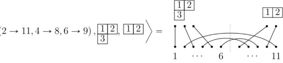
Vectors (3.29) admit a graphical presentation in terms of the so-called ‘partial one-row’ diagrams [CDDM], see Fig. 1.1.
ˇ ˇ ˇ ˇp2 Ñ 11, 4 Ñ 8, 6 Ñ 9q , 1 23 , 1 2 F “ • • • • • • • • • • • • • • • • 1 . . . 6 . . . 11 1 2 3 1 2
Figure 1.1: an example of a vector for B6,5p q.
Extending the terminology for the walled diagrams, we call lines, starting at tableaux, ‘propagating lines’ of the partial one-row diagram; other lines will of course be called ‘arcs’. We shall define the action of the algebra Br,sp q on the vector space Cr,sp fq. To this end,
it is sufficient to define the action of a walled diagram d from Br,sp q on a partial one-row
diagram vf with f arcs. Place d under vf and identify the nodes of vf with the corresponding
nodes in the top row of d. This is not necessarily a partial one-row diagram: two propagating lines might start to form an arc. In this case the result of action is zero. Otherwise, let ` be the number of closed loops obtained after the above identification. Omitting the loops we obtain some one-row diagram ¯vf. The diagram ¯vf may also contain intersections of
propagating lines. We numerate the propagating lines of vf by 1, . . . r´ f on the left of
the wall and by 1, . . . s´ f on the right. Let ⇡L and ⇡Rbe permutations of 1, . . . r´ f and
1, . . . s´ f respectively such that the application of ⇡L⇡R to the propagating lines’ ends of
vf gives ¯vf. The result of the action of d on vf is the combination of the partial one-row
diagrams obtained from ¯vf by forgetting the intersections of propagating lines and writing
out the result of the action ⇡L
ˇ ˇtL f ↵ and ⇡R ˇ ˇtR f ↵
on the vectors of the modules Sp L fq and
Sp R fq.
Consider the following vector in the module Cr,sp fq
vf “
ˇ
ˇpr Ñ r ` 1, r ´ 1 Ñ r ` 2, . . . , r ´ f ` 1 Ñ r ` fq, ˇtL
f, ˇtRf y, (3.30)
where ˇtL
f and ˇtRf are filled with numbers 1 . . . r´ f and 1 . . . s ´ f, respectively, in natural
ˇ ˇ ˇ ˇp4 Ñ 9, 5 Ñ 8, 6 Ñ 7q , 1 32 , 1 2 F “ 1 . . . 6 . . . 11 • • • • • • • • • • • • • • • • 1 3 2 1 2
Figure 1.2: the vector v3 for B6,5p q
Consider the set ShLr´f,f Ä SL
r (respectively, ShRf,s´f Ä SRs) of words r1 ` i1, 1sr2 `
i2, 2s . . . rr ´ f ` ir´f, r´ fs with ´1 § i1§ i2§ ¨ ¨ ¨ § ir´f † f (respectively, rr ` 1 ` jf, r`
1s . . . rr ` f ` j1, r` fs with ´1 § jf § ¨ ¨ ¨ § j1 § s ´ f). The elements of the set ShLr´f,f
(respectively, ShRf,s´f) represent pr ´ f, fq-shu✏es (respectively, pf, s ´ fq-shu✏es). Let SL
f Ä SLr (respectively, SRf Ä SRs) be a subset of all monomials in SLr which include
only generators sr´f`1, . . . , sr´1(respectively, sr`1, . . . , sr`f´1) for f ° 0. We suppose SL0 “
t1u and SR
0 “ t1u. In other words, the elements of SLf (respectively, SRf) are permutations
of the nodestr ´ f ` 1, . . . , ru (respectively, tr ` 1, . . . , r ` fu).
Let ⇥f with f • 0 denote the following set of permutations from Srˆ Ss:
⇥f “ ShLr´f,fSLfShRf,s´f. (3.31)
It is straightforward to see that the cardinality of ⇥f is
ˆ r f ˙ ˆ s f ˙ f !.
The set ⇥f contains those and only those permutations, from Sr ˆ Ss, of the nodes
of the partial one-row diagram corresponding to the vector vf which do not permute the
propagating lines of the diagram. Thus ⇥fproduces all possible subsets l1and l of cardinality
f and isomorphisms l1 Ñ l as in (3.29), i.e.
⇥fvf “ ˇˇl1Ñ l, ˇtLf, ˇtRf
↵(
. (3.32)
Let ⌃L
f (respectively, ⌃Rf) be the set of all permutations of t1, . . . , r ´ fu (respectively,
tr ` f ` 1, . . . , r ` su) such that LˇtLf and RˇtRf reproduce all possible standard tableaux.
Let ⌃f be the set constituted by permutations “ L R with L P ⌃Lf and R P ⌃Rf. In
particular, #⌃f “ dim Sp Lfq dim Sp Rfq.
We introduced the sets ⌃L
f and ⌃Rf in order to generate vectors (3.29) with all possible
standard tableaux. Namely, define the set Xf of permutations from Srˆ Ss
Xf “ ⇥f⌃f. (3.33)
Lemma 1.3.3 The set of vectors Xfvf forms a basis of Cr,sp fq. We have
dim Cr,sp fq “ #Xf “ ˆ r f ˙ ˆ s f ˙ f ! dim Sp Lfq dim Sp Rfq. (3.34)
1.3.4
Annihilator ideal
We proceed by describing the ideal annihilating the vector vf P Cr,sp fq. The basis Br,s will
be convenient for that purpose. We associate to any monomial
x“ rr ` i1, r´ j1s rr ` i2, r´ j2s . . . rr ` if, r´ jfs P Dpfqr,s (3.35)
the element
$pxq :“ rr ` i1, r´ j1s rr ` i2, r´ j2s . . . rr ` if, r` 1s . (3.36)
We denote by ¯Dpfqr,s the image of the set Dpfqr,s,
¯
Dpfqr,s :“ $pxq | x P Dpfqr,s(.
In words, to construct elements in ¯Dpfqr,s we delete the ends rr, r ´ jfs of the monomials in
Dpfqr,s.
Note that 0 § i1 † i2 † . . . † if † r and s ° j1 ° j2 ° . . . ° jf • 0 for an element
x P Dpfqr,s so 0§ i1 † i2 † . . . † if † r and s ° j1 ° j2 ° . . . ° jf´1 ° 0 for the element
(3.36).
We define the product of an element
y“ rr ` i1, r´ j1s . . . rr ` if, r` 1s P ¯Dpfqr,s
and the monomial rr, r ´ ks, k • 0, to be y˚ rr, r ´ ks :“
"
rr ` i1, r´ j1s . . . rr ` if, r´ ks if jf´1° k ,
? otherwise .
We introduce the sets
¯
Bptqr,s “ SLrD¯ptqr,s, t“ 1 . . . minpr, sq. (3.37) We describe the basis of the annihilator ideal of the vector vf in three steps.
Part 1. Let us introduce the following sets of elements of the algebra Br,sp q:
§f´1 i“0 ` rr, r ´ is rr ` i, r ` 1s´1´ ˘, (3.38) §minpf,s´1q´1 i“0 ` rr, r ´ is rr ` i ` 1, r ` 1s´1´ 1˘, (3.39) §minpf,r´1q i“1 ` rr, r ´ is rr ` i ´ 1, r ` 1s´1´ 1˘, (3.40) rr, r ´ fs rr ` f, r ` 1s´1. (3.41)
The elements (3.38)-(3.41) annihilate the vector vfwhich is clear from the following schematic
representation in terms of partial one-row diagrams:
. . . • • • • • • . . . • • • • • • ´ ¨ . . . • • • • • • . . . “ 0 , . . . • • • • • • . . . • • • • • • ´ . . . • • • • • • . . . “ 0 , . . . • • • • • • . . . • • • • • • ´ . . . • • • • • • . . . “ 0 , . . . • • • • • • • • . . . “ 0 . • • • • • • • • Let ⌥k
f Ä ShRf,s´fSRf⌃Rf be a subset of all monomials in SRs which include only generators
sr`k, . . . , sr`s´1. For brevity denote byJr ` 1Kpiq for i“ 1 . . . f the set of words
rr ` 1 ` k1, r` 1s . . . rr ` i ` ki, r` is, 0 § k1† s ´ 1, . . . , 0 § ki † s ´ i. (3.42)
We construct the following sets (t“ 1 . . . minpr, sq) of elements of the algebra Br,sp q: ¯ Bptqr,s˚§f´1 i“0 ` rr, r ´ isJr ` 1Kpiq´ ˘⌥i`2 f , (3.43) ¯ Bptqr,s˚§minpf,s´1q´1 i“0 ` rr, r ´ isJr ` 1Kpi`1q´ 1˘⌥i`2 f , (3.44) ¯ Bptqr,s˚§minpf,r´1q i“1 §r j“i`1 ` rr, j ´ isJr ` 1Kpi´1q´ 1˘⌥i`1 f , (3.45) ¯ Bptqr,s˚ rr, r ´ fsJr ` 1Kpfq⌥f`1f . (3.46)
A direct inspection shows that the elements (3.43)-(3.46) annihilate the vector vf since the
elements (3.38)-(3.41) do.
Part 2 Consider the settsr`i´ sr´i, i“ 1, . . . , f ´ 1u. The elements of this set annihilate
the vector vf, see figure below
. . . • • . . . • • . . . • • • • . . . • • . . . • • . . . ´ “ 0 . • • • • Given a word x in SR
fzt1u let sr`i be its leftmost generator (i“ 1 . . . f ´ 1). Denote by xc
the element of the algebra Br,sp q obtained by replacing the letter sr`i in the word x by the
combination psr`i´ sr´iq. Define the set SRf constituted by elements xc, xP SRfzt1u. The
elements of the set
⇥fS R
f⌃f (3.47)
annihilate the vector vf as well.
Part 3 We recall some results from [P]. Let Sp q be the Specht module for the symmetric group Sn for some n. Consider the vector in Sp q corresponding to the tableau ˇt filled with numbers 1 . . . n in natural order reading down the column from left to right. The annihilator ideal of ˇt is the left ideal generated by the Garnir elements and 1` ⌧ where ⌧ are transpositions in the column stabiliser of the tableau.
Denote gL
f (respectively, gRf) a basis of the annihilator ideal of the vector ˇtLf in S
` L f ˘ (respectively, ˇtR f in S ` R f ˘
). The following elements of the algebra Br,sp q
SLrDpfqr,sShf,s´fR SRfgRf, (3.48) ⇥fSRf ` gL f⌃Rf Y ⌃LfgRf Y gLfgRf ˘ . (3.49)
Let Af be the union of all sets (3.43)-(3.46), (3.47), (3.48), (3.49). The following Lemma
holds.
Lemma 1.3.5 The set Af is a basis of annihilator ideal of the vector vf,
#Af “ dim Br,sp q ´ dim Cr,sp fq. (3.50)
Proof. First let us show that the sets (3.43)-(3.46) and (3.48) are linearly independent. For that purpose consider the ‘higher’ terms in (3.43)-(3.45):
¯ Bptqr,s˚§f´1 i“0 ` rr, r ´ isJr ` 1Kpiq˘⌥i`2 f , (3.51) ¯ Bptqr,s˚§minpf,s´1q´1 i“0 ` rr, r ´ isJr ` 1Kpi`1q˘⌥i`2 f , (3.52) ¯ Bptqr,s˚§minpf,r´1q i“1 §r j“i`1 ` rr, j ´ isJr ` 1Kpi´1q˘⌥i`1 f . (3.53) Let Mip1q :“ ¯Bptqr,s˚`rr, r ´ isJr ` 1Kpiq˘⌥if`2 ,
so that the set in (3.51) is the union of sets Mi, i“ 0, 1, . . . , f ´ 1. Similarly, let
Mip2q:“ ¯Bptqr,s˚`rr, r ´ isJr ` 1Kpi`1q˘⌥if`2, and Mip3q:“ ¯Bptqr,s˚§r j“i`1 ` rr, j ´ isJr ` 1Kpi´1q˘⌥if`1. The union of sets Mip1q, Mip2q and Mip3q for fixed i (0§ i † f) is
¯ Bptqr,s˚ rr, r ´ is ˜ Jr ` 1Kpiq⌥if`2Y Jr ` 1Kpi`1q⌥if`2Y ˜ i § k“1 Jr ` 1Kpk´1q⌥kf`1 ¸¸ “ ¯Bptqr,s˚ rr, r ´ is ⌥1f, t“ 1 . . . minpr, sq. (3.54) For i“ f there are no sets (3.51) and (3.52); the union of Mfp1qand the set (3.46) is, similarly to (3.54):
¯
Bptqr,s˚ rr, r ´ fs ⌥1
f, t“ 1 . . . minpr, sq. (3.55)
It follows from the definition of ¯Bptqr,sthat the union of the expressions (3.54) for i“ 0 . . . f ´1
and (3.55) forms a subset SL
rDptqr,s⌥1f Ä Bptqr,s, thus the expressions (3.54) for i“ 0 . . . f ´1 and
(3.55) are linearly independent. Moreover, we have, by construction, ⌥1 f “ Sh
R
The union of the expressions (3.48), (3.54) and (3.55) over t “ 1 . . . minpr, sq and i “ 0 . . . f will be denoted by B. Since, by [P], the elements of gL
f (respectively, gRf) and ⌃Lf
(respectively, ⌃R
f) together form a basis in Sr (respectively, Ss), we conclude that B is
a linearly independent set. The same is true for the expressions (3.43)-(3.46) and (3.48). Indeed, each element in (3.43)-(3.45) is a combination of two monomials: the first one is a minimal word and contains more letters srthan the second. The number of occurrences of the
letter sr in a word defines a filtration on the algebra Br,sp q. Assume that the expressions
(3.43)-(3.46) and (3.48) are not linearly independent. Choose then a shortest non-trivial linear dependency. The coefficients of the words containing the maximal number of letters sr are zero (because these are the ones fromB) contradicting to the minimality of length of
of dependency.
Each expression (3.47) is a sum of two words from the set ⇥fSRf⌃f, one containing more
generators from SR
r than the other. This implies the linear independence of the set (3.47).
Next, we move to showing that the union of the sets (3.47) and (3.49) is linearly inde-pendent. First, note that replacing in the expressions (3.47) the elements from SRf by their pullbacks from SR
fzt1u we obtain a set N whose union with the expressions (3.49) is disjoint
and equals`⇥fSRf⌃f
˘
zXf. The set ⇥fSRf⌃f is a basis inC rSrˆ Sss. Therefore the union
of the sets N and (3.49) is linearly independent. The argument appealing to the length, defined by the number of generators from SR
r, completes the proof of the linear independence
of union of the sets (3.47) and (3.49).
The expressions from the sets (3.47) and (3.49) do not contain generators srand therefore
the whole set Af is linearly independent.
To calculate #Af, note that:
a) #B “ pr ` sq! ´ r!s! because B “ Br,szBp0qr,s,
b) the cardinality of the union of the sets (3.47) and (3.49) is r!s!´ dim Cr,sp fq (see
Lemma 1.3.3).
As a result, we arrive at the correct cardinality for the annihilator ideal #A“ dim Br,sp q ´
dim Cr,sp fq.
Lemmas 1.3.3 and 1.3.5 together provide a constructive proof of the following Theorem. Theorem 1.3.6 Fix a Br,sp q-module Cr,sp fq. Let Af and Xf be the sets given in lemmas
1.3.3 and 1.3.5. Then the union AfY Xf is a basis of the algebra Br,sp q.
1.3.7
Gelfand-Zetlin basis
The walled Brauer algebra Br,sp q is semisimple if and only if one of the following conditions
r“ 0 or s “ 0, R Z,
| | ° r ` s ´ 2,
“ 0 and pr, sq P tp1, 2q, p1, 3q, p2, 1q, p3, 1qu.
In this section we assume that is generic, that is, the walled Brauer algebra is semisimple. Let Au be the subalgebra in the algebra Br,sp q generated by the walled diagrams
non-trivial only at the first u sites of the sets pu
r,s and pdr,s (that is, to the right of the u-th
site the diagram has only vertical segments). For u § r, the algebra Au is isomorphic to
Bu,0p q ” CrSus while for r † u § r ` s the algebra Au is isomorphic to Br,u´rp q. The
algebras Au, 0§ u § r ` s, form an ascending chain of algebras
C ” A0Ä A1Ä . . . Ä Ar`s” Br,sp q . (3.56)
Let Cup q be a Au-module. We have (see [CDDM])
ResAu
Au´1Cup q »
à
µ
Cu´1pµq (3.57)
where the sum runs over all bipartitions µ such that is obtained from µ by • adding a box to the first diagram in the bipartition µ when 1 § u § r;
• adding a box to the second diagram or by removing a box from the first diagram when r` 1 § u § r ` s.
The formula (3.57) represents the branching rules for Br,sp q and defines the corresponding
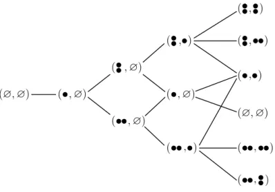
Bratelli diagram. Here is the figure showing the Bratteli diagram for the chain on the example of the walled Brauer algebra B2,2p q.
p?, ?q ( ,?q ( ,?q ( ,?q ( ,?q ( , ) ( , ) p?, ?q ( , ) ( , ) ( , ) ( , ) ( , )
Figure 1.3: Bratteli diagram
Define a standard walled -tableau as a sequence T “ p p0q, . . . , pr`sqq of bipartitions such that p0q “ p?, ?q, pr`sq “ and for each k “ 1, . . . , r ` s the bipartition pkq is obtained from pk´1q by the rules described above. Thus, T represents a path in the Bratteli diagram of the algebra Br,sp q.
We say that r` s is the length of T . We write U Õ T if the standard walled tableau U of length r` s ´ 1 is obtained by removing the last entry pr`sq from the sequence T . We shall denote byT the set of all standard walled -tableaux.
Since the branching rules for the Bratteli diagram are simple, we obtain a canonical decomposition of a simple Br,sp q-module Cr,sp q into a direct sum of simple A0-module, i.e.
1-dimensional subspaces
Cr,sp q “
à
T
VT,
where the sum runs over all standard walled -tableaux. Choose an arbitrary non-zero vector vT P VT. The vectors tvTu, T P T , form a basis of Cr,sp q, called the Gelfand-Zetlin
basis of Cr,sp q.
To each standard walled tableau T we attach its sequence of contentspc1pT q, . . . , cr`spT qq,
where
ckpT q “ j ´ i (3.58)
if 1§ k § r and pkq is obtained from pk´1q by adding a boxpi, jq to the first diagram in the bipartition,
if k• r ` 1 and pkq is obtained from pk´1qby removing a boxpi, jq from the first diagram,
ckpT q “ pj ´ iq ` (3.60)
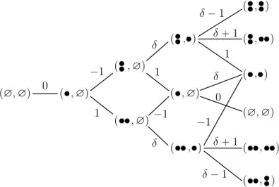
if k• r ` 1 and pkq is obtained from pk´1q by adding a boxpi, jq to the second diagram. It is convenient to decorate the Bratteli diagram, writing at each edge of the path T the corresponding content, as shown below on our example of the algebra B2,2p q.
p?, ?q ( ,?q ( ,?q ( ,?q ( ,?q ( , ) ( , ) p?, ?q ( , ) ( , ) ( , ) ( , ) ( , ) 0 ´1 1 1 ´1 ´ 1 ` 1 1 0 ` 1 ´ 1 ´1
Figure 1.4: Paths and contents
Clearly, a path T can be reconstructed from its sequence of contents.
We encode the sequence T of bipartitions in the following way. We first associate to the sequence T three Young diagrams 1pT q, ⌫pT q and 2pT q such that ⌫pT q Ñ 1pT q. The diagram 1pT q :“ prqL is the left diagram in the bipartition prq. The diagram ⌫pT q :“ pr`sqL is the left final diagram and the diagram 2pT q :“ pr`sqR is the right final diagram in the bipartition pr`sq. We call
DT :“ r 1pT q, ⌫pT q, 2pT qs
the triple diagram corresponding to the path T .
Next, we fill the boxes of the diagrams 1pT q, 2pT q and the set-theoretical di↵erence
1pT qz⌫pT q. Exactly as for the symmetric group, the boxes of the diagram 1pT q are filled
with numbers 1, . . . , r, representing the order in which the boxes were added in the se-quencep p0qL , . . . , prqL q. The boxes of the union` 1pT qz⌫pT q˘\ 2pT q are filled with numbers
r` 1, . . . , r ` s in the order in which the boxes were removed or added in the sequence p pr`1q, . . . , pr`sqq. The resulting filling we call the standard triple tableau WT
correspond-ing to the path T .
It is straightforward to see that the correspondence between the set of all paths and the set of all standard triple tableaux is one to one.
We visualize the standard triple tableau by putting the numbers corresponding to the filling of 1pT q in the upper left corner of boxes and the numbers corresponding to the filling of 1pT qz⌫pT q in the lower right corners. This should be clear on the following example of a path for the algebra B3,5p q.
Example 1.3.7.1 For the sequence T ”`
?, ?˘,` ,?˘,` ,?˘,` ,?˘,` , ˘,` , ˘,` , ˘,` , ˘,` , ˘ı
the corresponding triple diagram isrp2, 1q, p1q, p2, 1qs and the standard triple tableau WT is
”1 2 6 3 7 , 4 5 8 ı .
The contents of boxes in the sets 1pT q, 1pT qz⌫pT q and 2pT q are calculated according to the formulas (3.58), (3.59) and (3.60) respectively. The content of the box occupied by the number j in the standard triple diagram corresponding to a path T will be denoted by cjpT q.
1.4
Jucys–Murphy elements
For convenience in the following two sections we denote the generator sr by d.
The Jucys–Murphy elements for the walled Brauer algebras are adapted to the chain (3.56).
Let si,k, where 1§ i † k § r or r`1 § i † k § r`s, and di,k, where 1§ i § r † k § r`s,
denote the following walled diagrams: . . . . . . . . . . . . . . . . . . . . . . . . 1 i k r r` 1 r` s , si,k“
. . . . . . . . . . . . . . . . . . . . . . . . 1 r r` 1 i k r` s , si,k“ . . . . . . . . . . . . . . . . . . . . . . . . 1 i r r` 1 k r` s . di,k “ In particular, si“ si,i`1, 1§ i † r or r † i † r ` s, d “ dr,r`1.
In terms of generators, the elements si,k and di,k can be written as
si,k“ sisi`1. . . sk´2sk´1sk´2. . . si`1si,
di,k“ sisi`1. . . sr´1sk´1sk´2. . . sr`1dsr`1. . . sk´2sk´1sr´1. . . si`1si.
The Jucys-Murphy elements for the walled Brauer algebra are (see [BS, SS, JK]):
xk“ $ ’ ’ ’ ’ ’ & ’ ’ ’ ’ ’ % kÿ´1 i“1 si,k if 1§ k § r , ´ r ÿ i“1 di,k` kÿ´1 i“r`1 si,k` if k• r ` 1 . (4.61)
In [JK] it was proved that for each kP Z•0 the element
xk1` ¨ ¨ ¨ ` xkr` p´1qk`1pxkr`1` ¨ ¨ ¨ ` xkr`sq belongs to the center of Br,sp q.
One checks that the element xk commutes with any element of the subalgebra Ak´1, see
(3.56). This implies that the elements x1,. . . , xr`s of Br,sp q pairwise commute. Moreover,
it follows from the representation theory of the walled Brauer algebras that the subalgebra generated by the elements x1, . . . , xr`s is a maximal commutative subalgebra of the algebra
Br,sp q. It is called the Gelfand-Zetlin subalgebra of Br,sp q.
It turns out that the vectors vT introduced in (1.3.7) are eigenvectors for the
Jucys-Murphy element xj, j “ 1, . . . , r ` s and the eigenvalues are precisely the contents,
1.5
Orthogonal primitive idempotents
1.5.1
Algebraic background
We remind some basic results from the theory of semisimple finite demensional algebras (for a brief introduction see [OP]). Let ApKq be a finite-dimensional unital associative algebra over a field K. Consider the regular left A-module Areg. Suppose Areg decomposes into a
direct sum of left A-modules Mi, i“ 1, . . . , k,
Areg “ k
à
i“1
Mi.
The subspaces MiÄ A are left ideals of A. The corresponding decomposition of unit element
of Areg is 1“ k ÿ i“1 ei where ei P Mi. (5.62)
It follows that eiej “ ijei and the elements teiusi“1 form the set of mutually orthogonal
idempotents in A. We have Areg “ k à i“1 Aei.
Thus, there is the one-to-one correspondence between the decompositions of the regular module Areg into a direct sum of submodules and the resolutions of the unit element of the
algebra A into a sum of mutually orthogonal idempotents.
The module Mi is indecomposable if and only if the corresponding idempotent cannot
be resolved into a sum of nontrivial mutually orthogonal idempotents. An idempotent pos-sessing this property is called ‘primitive idempotent’.
Further, we recall some standard facts valid in the situation when the branching rules are simple and the vectors vT are common eigenvectors of a set of elements generating a
maximal commutative subalgebra.
Since the vectors vT, T P T , form a basis of Cr,sp q, we have the complete set tETu
of primitive idempotents in MatpCr,sp qq; the operator ET is the projector on the
one-dimensional subspace VT along the subspace of codimension one spanned by the vectors vT1,
T1 P T ztT u. The primitive idempotent ET, corresponding to the vector vT, satisfies
xtET “ ETxt“ ctpT qET , t“ 1, . . . , r ` s . (5.63)
Consider the standard walled tableau U “ p p0q, . . . , pr`s´1qq; recall that we assume that s° 0.
For a Young diagram we let
Ap q be the set of all addable cells and
Rp q the set of all removable cells .
Let ↵ P R`⌫pUq˘\ A` 2pUq˘ be the box of WT occupied by the number r` s. By
construction, we have
ET “ EU px
r`s´ a1q . . . pxr`s´ a`q
pcr`spT q ´ a1q . . . pcr`spT q ´ a`q
, (5.64)
where a1, . . . , a` are the contents of all boxes in
ˆ
R`⌫pUq˘\ A` 2pUq˘ ˙
zt↵u.
The elementstETu for T a standard walled -tableau, P ⇤r,s, form a complete set of
pairwise orthogonal primitive idempotents for Br,sp q.
The relation (5.64) can be written in the form ET “ EU u´ cr`s u´ xr`s ˇ ˇ ˇ u“cr`s , (5.65)
where u is a complex variable. Indeed, the actions of the right hand sides of (5.64) and (5.65) on the vectors vT, T P T , coincide.
Given a standard walled tableau U “ p p0q, . . . , pr`s´1qq, we have EU “
ÿ
T :UÕT
ET . (5.66)
1.5.2
Fusion procedure for the walled Brauer algebra
A fusion procedure gives a construction of the maximal family of pairwise orthogonal minimal idempotents in the algebra.
The fusion procedure (for the symmetric group) originates in the work of Jucys [19], see also the subsequent works [Ch, Na, GP]. A simplified version of the fusion procedure for the symmetric group involving the consecutive evaluation was suggested by Molev in [Mo]. Later the analogues of this simplified fusion procedure were suggested for the Hecke algebra [IMOs], for the Brauer algebra [IM, IMO], for the complex reflection groups of type Gpm, 1, nq, for the cyclotomic Hecke algebras [OP1, OP2], for the cyclotomic Brauer algebras [C], for the
Birman–Murakami–Wenzl algebras [IMO2]. In [OP3] this fusion procedure was applied for the calculation of weights of certain Markov traces on the cyclotomic Hecke algebras.
The fusion procedure is closely related with the inductive approach to the representation theory of towers of algebras, see [OV] for the symmetric groups, and the generalizations for the Hecke algebra [IO], for the cyclotomic Hecke algebra [OP4], complex reflection groups [OP5] and Brauer algebras [IO2].
Spectral parameters
To shorten the formulation of our results it is convenient to introduce the following function on the sett1, . . . , r ` su "pjq “ # 0 if j § r , 1 if j ° r . (5.67) Denote, for i‰ j, si,jpuq “ 1 ´ si,j u if "piq ` "pjq is even , di,jpuq “ 1 ´ di,j u if "piq ` "pjq is odd .
Let wi,jpuq be, depending on "piq ` "pjq, either si,jpuq or di,jpuq. If the indices i, j, k, l are
pairwise distinct then
wi,jpuqwk,lpvq “ wk,lpvqwi,jpuq . (5.68)
We have
si,jpuqsi,jp´uq “
u2´ 1
u2 , (5.69)
and
di,jpuqdi,jp ´ uq “ 1 . (5.70)
The functions si,jpuq satisfy the Yang-Baxter equation with the spectral parameter
si,jpuqsi,kpu ` vqsj,kpvq “ sj,kpvqsi,kpu ` vqsi,jpuq , (5.71)
with pairwise distinct indices i, j, k. Additionally, we have (i‰ j ‰ k ‰ i)
dj,ipuqdk,ipu ´ vqsj,kpvq “ sj,kpvqdk,ipu ´ vqdj,ipuq , (5.72)
and
Remark. Equations (5.71), (5.72) and (5.73) can be elegantly written in a uniform manner. Let
˜
wi,jpuq :“
"
si,jpuq if "piq ` "pjq is even ,
di,jp {2 ´ uq if "piq ` "pjq is odd .
Then
˜
wi,jpuq ˜wi,kpu ` vq ˜wj,kpvq “ ˜wj,kpvq ˜wi,kpu ` vq ˜wi,jpuq
whenever i‰ j ‰ k ‰ i. First fusion procedure
The original fusion procedure for the Brauer algebra was given in [IM]. In this section we formulate its analogue for the walled Brauer algebra.
In what follows we let
n“ r ` s .
Consider the rational function, in variables u1, . . . , un, with values in the walled Brauer
algebra Br,sp q: r,s :“ Dr,sSr˚Ss , (5.74) where Dr,s :“ π 1§i§r r`1§j§n di,jpui` ujq and Sr :“ π 1§i†j§r si,jpui´ ujq , ˚Ss :“ π r`1§i†j§n si,jpui´ ujq . (5.75)
The products in the definitions ofDr,s, Sr and ˚Ssare calculated in the lexicographical order
on the pairspi, jq (that is, pi1, j1q precedes pi2, j2q if i1† i2or i1“ i2 and j1† j2).
Let T “ p p0q, . . . , pnqq, pnq “ P ⇤r,s, be a standard walled -tableau describing a
path in the Bratteli diagram for the walled Brauer algebra Br,sp q. We define the rational
function in the variables u1, . . . , un:
zT :“ n π i“1 ui´ ci ui´ "piq ˆ π 1§j†i§r or r†j†i§n pui´ ujq2 pui´ ujq2´ 1 , (5.76)
where the function " is defined by (5.67), and for brevity we denoted ci“ cipT q, i “ 1, . . . , n.
Set
Theorem 1.5.3 The primitive idempotent ET, corresponding to the standard walled
-tableau T , is found by the consecutive evaluations ET “ Tpu1, . . . , unq ˇ ˇ u1“c1 ˇ ˇ u2“c2. . . ˇ ˇ un“cn .
Example 1.5.3.1 For r“ s “ 2, let T be the standard walled tableau corresponding to the contents sequence p0, ´1, 1, 0q, see Figure 1.4. We have
p0, u2, u3, u4q “ ˆ 1´ d1,3 u3 ˙ ˆ 1´ d1,4 u4 ˙ ˆ 1´ d u2` u3 ˙ ˆ 1´ d2,4 u2` u4 ˙ ˆ ˆ 1` s1 u2 ˙ ˆ 1´ s3 u3´ u4 ˙ .
This expression has singularities at u3 “ ´u2 or u4 “ 0. However in the process of the
consecutive evaluations of the product of pu1, u2, u3, u4q with the prefactor zpu1, u2, u3, u4q
the singularities cancel and we find ET “
1
2 p ´ 1qp1 ´ s1q ¨ ds1s3d¨ p1 ´ s1q . Remark. The function
π 1§i†j§n di,jpui` ujq π 1§i†j§n si,jpui´ ujq (5.78)
for the Brauer algebra Bnp q was suggested in [Na2]. Note that the function r,s, defined
in (5.74), can be obtained by dropping in the expression (5.78) factors corresponding to the diagrams which do not exist in the walled Brauer algebra. Thus the function r,s makes
sense in the Brauer algebra Bnp q and the consecutive evaluations of the product zT ¨ r,s
give rise to certain idempotents of the Brauer algebra Bnp q. It would be interesting to
understand the representation-theoretic/combinatorial meaning of these idempotents. Reformulation of Theorem 1.5.3
As we already stressed, we are interested in the fusion procedure only after the wall crossing so we shall accordingly change the notation. A standard walled -tableau T “ p p0q, . . . , pr`sqq,
pr`sq“ , will be denoted by T “ pT
r, pr`1q, . . . , pr`sqq where Tr “ p p0q, . . . , prqq is the
standard Young tableau of shape 1pT q. We fix the tableau T till the end of Section and set ci“ cipT q.
For j such that r` s • j ° r let dÓj :“ dr,jpur` ujqdr´1,jpur´1` ujq . . . d1,jpu1` ujq and ˚dÓ j :“ dÓj ˇ ˇ u1“c1. . . ˇ ˇ ur“cr “ dr,jpcr` ujqdr´1,jpcr´1` ujq . . . d1,jpc1` ujq .
The symbol˚(it appeared already in (5.74)) over a letter signifies that we are dealing with a rational function which depends only on the variables ur`1, . . . , un.
With the help of the equalities (5.72), one finds
Dr,sSr “ SrdÓr`1dÓr`2. . . dÓn .
The fusion procedure of [Mo] for the symmetric group says that the primitive idempotent ETr corresponding to the standard tableau Tr of the symmetric groupSr is obtained by the
consecutive evaluations ETr “ ˜ r π i“1 ui´ ci ui ˆ π 1§j†i§r pui´ ujq2 pui´ ujq2´ 1¨ Sr ¸ ˇˇ ˇ ˇ u1“c1 . . . ˇ ˇ ˇ ˇ ur“cr .
The part of the prefactor zT, see (5.76), which corresponds to the after-wall tailp. . . , pr`1q, . . . , pr`sqq
of the tableau T , is the rational function in the variables ur`1, . . . , un:
˚zT :“ n π i“1 ui´ ci ui´ ˆ π r†j†i§n pui´ ujq2 pui´ ujq2´ 1 . Let now ˚n;T rpur`1, . . . , unq :“ ETr˚d Ó r`1˚dÓr`2. . .˚dÓnS˚s and ˚Tpur`1, . . . , unq :“ ˚zT ¨ ˚n;T rpur`1, . . . , unq .
We reformulate Theorem 1.5.3 in the following way: the idempotent ET is found by the
consecutive evaluations ET “ ˚Tpur`1, . . . , unq ˇ ˇ ur`1“cr`1. . . ˇ ˇ un“cn .
Proof of Theorem 1.5.3
We repeat that we assume that s° 0 because before crossing the wall our formulas reproduce the formulas for the symmetric groups from [Mo].
We shall often write di,jpu, vq and si,jpu, vq instead of di,jpu ` vq and si,jpu ´ vq.
We rewrite the function r,s, defined by (5.74), in the form adapted to the consecutive
evaluations. Let
n:“ dr,npur, unq . . . d1,npu1, unq ¨ sr`1,npur`1, unq . . . sn´1,npun´1, unq . (5.79)
Lemma 1.5.4 We have
r,s“ r,s´1¨ n .
Proof. Clearly,Dr,s “ Dr,s´1¨d1,npu1, unq . . . dr,npur, unq. The Yang–Baxter equations (5.72)
imply the identity
d1,npu1, unq . . . dr,npur, unq ¨ Sr “ Sr¨ dr,npur, unq . . . d1,npu1, unq .
The well-known equality ˚Ss “ ˚Ss´1¨ sr`1,npur`1, unq . . . sn´1,npun´1, unq and the
commuta-tivity relation
dr,npur, unq . . . d1,npu1, unq ¨ ˚Ss´1“ ˚Ss´1¨ dr,npur, unq . . . d1,npu1, unq ,
complete the proof.
We first analyze what happens when we cross the wall.
Lemma 1.5.5 Let U be a standard walled tableau for the algebra Br,0p q, that is, for the
symmetric group Sr. The following identity holds in the walled Brauer algebra Br,1p q:
EU¨ d1,r`1pw ´ c1q . . . dr,r`1pw ´ crq “
w´ ` xr`1
w ¨ EU , (5.80)
where ci“ cipUq, i “ 1, . . . , r.
Proof. The proof is by induction in r. The induction base, for the algebra B1,1p q, is
straightforward.
Let W Õ U. By the recursive construction of the primitive idempotents for the sym-metric group in [Mo] (which is exactly the ‘before the wall’ part of our formula), we have