Combining approaches for predicting genomic evolution

HAL Id: tel-01428885

https://tel.archives-ouvertes.fr/tel-01428885

Submitted on 6 Jan 2017

HAL is a multi-disciplinary open access

archive for the deposit and dissemination of sci-entific research documents, whether they are pub-lished or not. The documents may come from teaching and research institutions in France or abroad, or from public or private research centers.

L’archive ouverte pluridisciplinaire HAL, est destinée au dépôt et à la diffusion de documents scientifiques de niveau recherche, publiés ou non, émanant des établissements d’enseignement et de recherche français ou étrangers, des laboratoires publics ou privés.

Combining approaches for predicting genomic evolution

Bassam Alkindy

To cite this version:

Bassam Alkindy. Combining approaches for predicting genomic evolution. Bioinformatics [q-bio.QM]. Université de Franche-Comté, 2015. English. �NNT : 2015BESA2012�. �tel-01428885�

é c o l e d o c t o r a l e _{s c i e n c e s p o u r l ’ i n g é n i e u r e t m i c r o t e c h n i q u e s}

Combining Approaches for

Predicting Genomic Evolution

Combinaison d’Approches pour Résoudre le Problème du

Réarrangement de Génomes

é c o l e d o c t o r a l e _{s c i e n c e s p o u r l ’ i n g é n i e u r e t m i c r o t e c h n i q u e s}

Combining Approaches for Predicting Genomic

Evolution

Combinaison d’Approches pour Résoudre le Problème du Réarrangement

de Génomes

A dissertation presented by

B

ASSAM

B

ASIM

J

AMIL

A

LKINDY

and submitted to the

University of Franche-Comté

in partial fulfillment of the Requirements for obtaining the degree

DOCTOR OF PHYLOSOPHY

in speciality ofComputer Science

Research Unit :

Laboratory of Femto-ST (SPIM)

Defended in public on 17 December 2015 in front of the Jury composed from :

LHASSANE IDOUMGHAR President of jury Professor, University of Haute-Alsace JEAN-PAULCOMET Reviewer Professor, University of Nice

STÉPHANECHRÉTIEN Reviewer Senior Researcher (HDR), National Physical

Laboratory Mathematics, Modelling, and Simulation, UK

CHRISTOPHEGUYEUX Examiner Professor, University of Franche-Comté

JACQUESM. BAHI Supervisor Professor, University of Franche-Comté

JEAN-FRANÇOISCOUCHOT Co-Supervisor MCF, University of Franche-Comté

MICHELSALOMON Co-Supervisor MCF, University of Franche-Comté

Acknowledgement

Following this work, I want to express my gratitude to allow all people who have con-tributed, each has its method, at the completion of this thesis. I want to express my deepest thanks to my supervisor Prof. Jacques M. Bahi and to my co-supervisors Dr. Jean-Francois Couchot and Dr. Michel Salomon. Words are broken me to express my gratitude. Their skills, their scientific rigidity, and clairvoyance taught me a lot. Indeed, I thank them for their organizations, and expert advice provide me they knew through-out these three years and also for their warm quality human, and in particular for the confidence they have granted to me.

I would nevertheless like to thank more particularly proudly Prof. Christophe Guyeux, professor in the University of Franche-Comté, for his advisers and his scientific expert who helped and guided me a lot for the completion of this thesis.

I would like to extend my sincere thanks to Lhassane Idoumghar, Professor at the Univer-sity of Haute-Alsace, for giving me the honor to president the jury. I also extend my sincere thanks to Jean-Paul Comet, Professor at the University of Nice and Stéphane Chrétien, MCF HDR, National Physical Laboratory Mathematics, Modelling, and Simulation, UK, for giving me the honor of accepting to be rapporteurs of this thesis. I would like to extend my sincere thank to the examiners: Christophe Guyeux, Professor at the University of Franche-Comté and Jean-Francois Couchot, MCF, University of Franche-Comté.

I extend my warmest thanks to the Minister of Higher Education and Scientific Research in Iraq represented by Campus France, the University of Mustansiriyah, and the University of Franche-Comté, for their co-operation to finance this thesis.

My gratitude and my thanks go to the crew members of AND for the friendly and warm atmosphere in which it supported me to work. Therefore thanks to Raphaël Couturier, Karine Deschinkel, Stephane Domas, Giersch Arnaud, Mourad Hakem, Ali Idrees Kad-hum, Ahmed Al-Badri, David Laiyamani, Yousra Ahmed Fadil, Abdallah Makhoul, Roxane Mallouhy, Ahmed Mostefaoui, and to whom I missed their names.

My gratitude and my thanks go to the crew members of DISC for the friendly and warm atmosphere in which it supported me to work. Therefore, Thanks Olga Kouchnarenko, di-rector of DISC (Informatique des systèmes complexes) department in Besançon, Pierre-Cyrille Héam, Dominique Menetrier, Jean-Michel Caricand, Laurent Steck and to all other people if I forget his name. For their unwavering support and encouragement.

I would also like express my strongly thanks to the crew of super-computer facili-ties (Mesocentre) for their generous advices and help in launching the calculations using supercomputer capabilities by installing the modules, creation the site Internet that make dreams come true. Therefore, thanks to Laurent Philippe, Kamel Mazouzi, Guillaume

vi

Laville, and Cédric Clerget.

I would also like express my thanks to my friends in bioinformatics team of Christophe for their kindly friendship, Thanks, Huda AL-NAYYEF, Bashar Al-Nauimi, Panisa Treep-ong. Before closing, I want to thank my dear friends including Lilia Ziane Khodja, Abbas Abdulhameed, Hamida Bouaziz, Hana M’Hemdi, Lemia Louail, Kitsiri Kizzyy Chochiang, who shared my hopes and studies, which made me comfort in the difficult moments and with whom I shared unforgettable moments of events.

Dedication

To my wife Huda, with my love. I am also addressing the strongest thanksgiving words to my parents, my wife’s parents, my sisters and their families, my brothers and their families, and to my lovely family, for their support and encouragement during the thesis in long years of studies. Their affection and trust lead me and guide me every day. Thank you, Mom, Dad, for making me what I am today.

Abstract

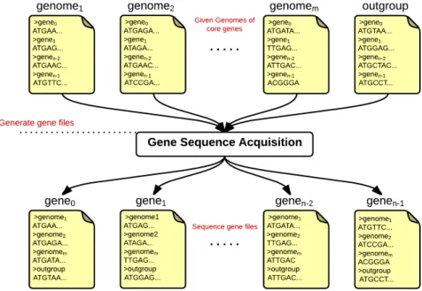
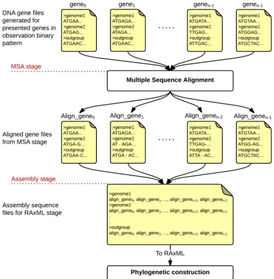
Chloroplasts is one of many types of organelles in the plant cell. They are considered to have originated from cyanobacteria through endosymbiosis, when an eukaryotic cell en-gulfed a photosynthesizing cyanobacterium, which remained and became a permanent resident in the cell. The term of chloroplast comes from the combination of plastid and chloro, meaning that it is an organelle found in plant cells that contains the chlorophyll. Chloroplast has the ability to convert water, light energy, and carbon dioxide (CO2) in chemical energy by using carbon-fixation cycle (also called Calvin Cycle, the whole pro-cess being called photosynthesis). This key role explains why chloroplasts are at the ba-sis of most trophic chains and are thus responsible for evolution and speciation. Moreover, as photosynthetic organisms release atmospheric oxygen when converting light energy in chemical one, and simultaneously produce organic molecules from carbon dioxide, they originated the breathable air and represent a mid to long term carbon storage medium. Consequently, exploring the evolutionary history of chloroplasts is of great interest, and we propose to investigate it by the mean of ancestral genomes reconstruction. This re-construction will be achieved in order to discover how the molecules have evolved over time, at which rate, and to determine whether evidences of their cyanobacteria origin can be presented by this way. This long-term objective necessitates numerous inter-mediate research advances. Among other things, it supposes to be able to apply the ancestral reconstruction on a well-supported phylogenetic tree of a representative collec-tion of chloroplastic genomes. Indeed, sister relacollec-tionship of two species must be clearly established before trying to reconstruct their ancestor. Additionally, it implies to be able to detect content evolution (modification of genomes like gene loss and gain) along this accurate tree. In other words, gene content evolution on the one hand, and accurate phylogenetic inference on the other hand, must be carefully regarded in the specific case of chloroplast sequences, as the two main prerequisites in our quest of the last universal common ancestor of these chloroplasts.

In detail, given a collection of genomes, it is possible to define their core genes as the common genes that are shared among all the species, while pan genome is all the genes that are present at least once (all the species have each core gene, while a pan gene is in at least one genome). The key idea behind identifying core and pan genes is to understand the evolutionary process among a given set of species: the common part (that is, the core genome) can be used when inferring the phylogenetic relationship, while accessory genes of pan genome explain to some extent each species specificity. In the case of chloroplasts, an important category of genome modification is indeed the loss of functional genes, either because they become ineffective or due to a transfer to the nucleus. Thereby a small number of gene loss among species may indicate that these species are close to each other and belong to a similar lineage, while a large loss means

x

distant lineages.

More precisely, a key idea concerning phylogenetic classification is that a given DNA mu-tation shared by at least two taxa has a larger probability to be inherited from a common ancestor than to have occurred independently. Thus shared changes in genomes allow to build relationships between species. In that case, homologous genes are genes derived from a single ancestral one. They are divided in two types, namely paralogous and or-thologous genes. Paralogy arises from ancestral gene duplication while the oror-thologous genes are products of speciation. Being able to understand the way that paralogous and orthologous genes evolve over time should clarify certain aspects of both the chloroplast evolution and origin.

We thus wonder, given a large set of complete chloroplastic genomes, how to find their genes and to determine how they have been acquired or lost during Evolution. Such a knowledge will lead to the ability to reconstruct the ancestral sequences of two sister species, using an algorithm to develop. Applying such an algorithm on a well supported tree will help us to reach the last common universal ancestor of all existing chloroplasts, and finally to study how these genomes have evolved over time.

Table of Contents

1.2 Presentation of the Problems . . . 2

1.3 Thesis Objective . . . 3

1.4 Contributions . . . 4

1.5 Publications . . . 4

1.5.1 Acts of selective international conferences . . . 4

1.5.2 Publications in national seminars and workshops . . . 5

1.6 List of Abbreviations . . . 6

1.7 Mathematical Notations . . . 7

1.8 Organization of the Thesis Manuscript . . . 7

I State of the Art 9 2 A short history regarding core and pan genome extraction 11 3 Technical Aspects of Sequence Alignments 13 3.1 Introduction . . . 13

3.2 Standard Substitution Matrices . . . 15

3.2.1 Nucleotide substitution matrices . . . 15

3.2.2 Point Accepted Mutation (PAM) matrix . . . 17

3.2.3 Blocks Substitution Matrix (BLOSUM) . . . 18 xi

xii TABLE OF CONTENTS

3.3 Local Alignment Algorithms . . . 20

3.3.1 Basic local alignment search tool (BLAST) . . . 20

3.3.2 Smith–Waterman algorithm . . . 21

3.4 Global Sequence Alignment: the Needleman Wunsch example . . . 23

3.5 Edit distances . . . 24

3.6 Multiple Sequence Alignment (MSA) . . . 25

3.7 Conclusion . . . 26

4 Concept of Phylogenetic Tree Construction 27 4.1 Various Types of Phylogenetic Trees . . . 27

4.2 Methods for Phylogenetic Construction . . . 30

4.2.1 Introduction . . . 30

4.2.2 A Distance-Based Method: the Neighbor-Joining Algorithm . . . 30

4.3 Character-Based Methods . . . 32 4.3.1 Maximum Parsimony . . . 32 4.3.2 Bayesian Method . . . 33 4.3.3 Maximum Likelihood . . . 33 4.3.3.1 General presentation . . . 33 4.3.3.2 Bootstrap values . . . 33

4.4 Stages for Phylogenetic Analysis . . . 34

4.5 Conclusion . . . 37

II Contributions 39 5 General Introduction 41 6 Core-Genes Prediction Approaches 43 6.1 Introduction . . . 43

6.2 Core genome extraction Approaches . . . 44

6.2.1 Similarity-based Approach . . . 44

6.2.1.1 Theoretical presentation . . . 45

6.2.1.2 A first case study . . . 46

6.2.2 Annotation-based Approach . . . 49

6.2.2.1 Using genes names provided by annotation tools . . . 49

6.2.2.2 Names processing . . . 50

TABLE OF CONTENTS xiii

6.2.3 Quality Test Approach . . . 52

6.2.3.1 Construction of quality genomes . . . 53

6.2.3.2 Core and pan genomes . . . 55

6.2.3.3 Execution time and memory usage . . . 59

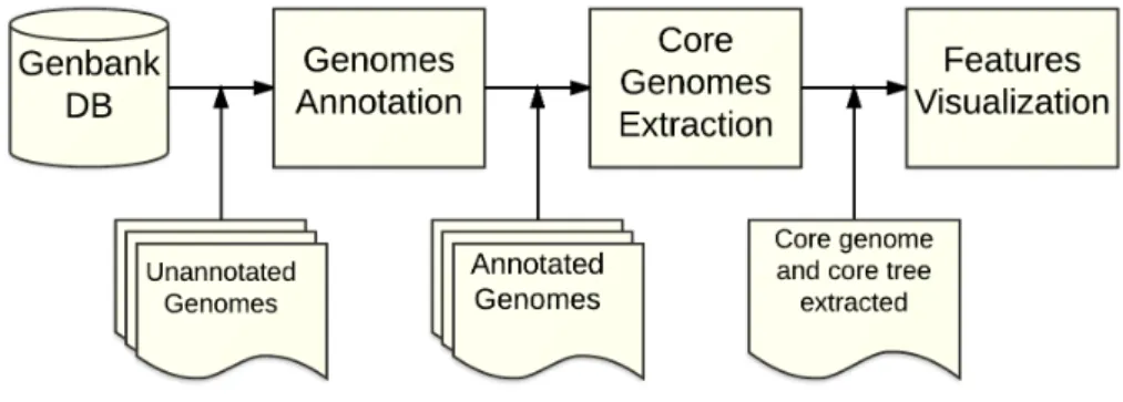
6.3 Features visualization . . . 61

6.3.1 The core tree . . . 61

6.3.2 A first phylogenetic study . . . 61

6.4 Discussion and biological evaluation . . . 65

6.5 Conclusion . . . 66

7 Inferring Phylogenetic Trees using Genetic Algorithm 69 7.1 General Presentation . . . 69

7.2 Presentation of the problem . . . 70

7.3 Generation of the initial population . . . 70

7.4 Genetic algorithm . . . 72

7.4.1 Genotype and fitness value . . . 72

7.4.2 Genetic process . . . 73

7.4.3 Crossover step . . . 74

7.4.4 Mutation step . . . 75

7.4.5 Random step . . . 76

7.5 Targeting problematic genes using statistical tests . . . 76

7.5.1 The Lasso test . . . 76

7.5.2 Second stage of genetic algorithm . . . 77

7.6 Case studies . . . 77

7.6.1 Pipeline evaluation by various groups of plant species . . . 77

7.6.2 Investigating Apiales order . . . 80

7.6.2.1 Method to select best topologies . . . 80

7.6.2.2 Topological Analysis . . . 81

7.7 Conclusion . . . 84

8 Inferring Phylogenetic Trees using DPSO 85 8.1 Discrete Particle Swarm Optimization . . . 85

8.2 Application to Phylogeny . . . 86

8.3 Experimental results and discussion . . . 89

8.3.1 Experimental protocol and results . . . 89

xiv TABLE OF CONTENTS

8.4 MPI: Proposed Methodology . . . 92

8.4.1 The master-slave proposal . . . 92

8.4.2 Distributed BPSO with MPI . . . 95

8.4.2.1 Distributed BPSO Algorithm: Version I . . . 95

8.4.2.2 Distributed BPSO Algorithm: Version II . . . 95

8.4.3 Genetic Algorithm vs Particle Swarm Algorithm . . . 95

8.5 Conclusion . . . 99

9 Ancestral Reconstruction 101 9.1 General Presentation of the Problem . . . 101

9.2 Ancestral Reconstruction Pipeline . . . 104

9.2.1 Data Preparation . . . 104

9.2.2 Ancestral Analysis Methods . . . 106

9.2.2.1 Ancestor Prediction based on Gene Contents . . . 106

9.2.2.2 Ancestor Prediction based on Sequence Comparison . . . 110

9.2.3 Ancestral Information . . . 112

9.3 Conclusion . . . 115

III Conclusion and Future Work 117 10 Conclusion 119 10.1 Conclusion . . . 119

CHAPTER

1

Introduction

1.1/

G

P

Chloroplasts are one of the main organelles in plant cell. They are considered to have originated from cyanobacteria through endosymbiosis, when an eukaryotic cell engulfed a photosynthesizing cyanobacterium, which remained and became a permanent resident in the cell. The term of chloroplast comes from the combination of plastid and chloro, meaning that it is an organelle found in plant cells that contains the chlorophyll. Chloro-plast has the ability to convert water, light energy, and carbon dioxide (CO2) in chemical

energy by using carbon-fixation cycle [1] (also called Calvin Cycle, the whole process being called photosynthesis). This key role explains why chloroplasts are at the basis of most trophic chains and are thus responsible for evolution and speciation. Moreover, as photosynthetic organisms release atmospheric oxygen when converting light energy in chemical one, and simultaneously produce organic molecules from carbon dioxide, they originated the breathable air and represent a mid to long term carbon storage medium. Consequently, exploring the evolutionary history of chloroplasts is of great interest, and we propose to investigate it by the mean of ancestral genomes reconstruction. This re-construction will be achieved in order to discover how the molecules have evolved over time, at which rate, and to determine whether evidences of their cyanobacteria origin can be presented by this way. This long-term objective necessitates numerous inter-mediate research advances. Among other things, it supposes to be able to apply the ancestral reconstruction on a well-supported phylogenetic tree of a representative collec-tion of chloroplastic genomes. Indeed, sister relacollec-tionship of two species must be clearly established before trying to reconstruct their ancestor. Additionally, it implies to be able to detect content evolution (modification of genomes like gene loss and gain) along this accurate tree. In other words, gene content evolution on the one hand, and accurate phylogenetic inference on the other hand, must be carefully regarded in the specific case of chloroplast sequences, as the two main prerequisites in our quest of the last universal common ancestor of these chloroplasts.

In detail, given a collection of genomes, it is possible to define their core genes as the common genes that are shared among all the species, while pan genome is all the genes

2 CHAPTER 1. INTRODUCTION

that are present at least once (all the species have each core gene, while a pan gene is in at least one genome). The key idea behind identifying core and pan genes is to understand the evolutionary process among a given set of species: the common part (that is, the core genome) can be used when inferring the phylogenetic relationship, while accessory genes of pan genome explain to some extent each species specificity. In the case of chloroplasts, an important category of genome modification is indeed the loss of functional genes, either because they become ineffective or due to a transfer to the nucleus. Thereby a small number of gene loss among species may indicate that these species are close to each other and belong to a similar lineage, while a large loss means distant lineages.

More precisely, a key idea concerning phylogenetic classification is that a given DNA mu-tation shared by at least two taxa has a larger probability to be inherited from a common ancestor than to have occurred independently. Thus shared changes in genomes allow to build relationships between species. In that case, homologous genes are genes derived from a single ancestral one. They are divided in two types, namely paralogous and or-thologous genes. Paralogy arises from ancestral gene duplication while the oror-thologous genes are products of speciation. Being able to understand the way that paralogous and orthologous genes evolve over time should clarify certain aspects of both the chloroplast evolution and origin.

We thus wonder, given a large set of complete chloroplastic genomes, how to find their genes and to determine how they have been acquired or lost during Evolution. Such a knowledge will lead to the ability to reconstruct the ancestral sequences of two sister species, using an algorithm to develop. Applying such an algorithm on a well supported tree will help us to reach the last common universal ancestor of all existing chloroplasts, and finally to study how these genomes have evolved over time.

1.2/

P

P

Understanding the evolution of DNA molecules is an open and complex problem.

Algorithms have been proposed to tackle this problem, but either they are limited to the evolution of one given character (for instance, a specific nucleotide), or conversely they theoretically focus on large scale nuclear genomes (several billions of nucleotides) facing multiple recombination events. One-character methods cannot be extended to large scale genomic evolution, while it is well known that the problem is NP hard when considering the set of all possible recombination on large genomes. So no concrete solution exists at present regarding the evolution of large DNA sequences. However, in this thesis, we focus on genomes that have a reasonable size and who faced a reasonable number of recombination. This is why we argue that the problem may be tractable in the chloroplast case – but it requires the design of ad hoc solutions, and various difficulties still remain to circumvent when dealing with such a specificity.

First, the evolution history of chloroplasts can only be inferred on shared coding se-quences, which are difficult to extract. Indeed, no tool is available to find the core genes, and so bioinformatics investigations using sequence annotation and comparison tools are required to be able to determine the core of chloroplast genomes for a given set of photosynthetic organisms. Additionally, the amount of completely sequenced chloroplast genomes increases rapidly, leading to the possibility to build large-scale phylogenies that

1.3. THESIS OBJECTIVE 3

represent well the plant diversity. But the size of the core genome is dramatically reduced when we consider very divergent plant species, which explain why these phylogenies are usually done using a small number of chloroplastic genes. In that case, we can wonder if we deal with a gene tree or a species one, and the obtained phylogeny is probably not accurate enough to deploy an ancestral reconstruction on it.

It is true that, if we are able to automatically consider various subsets of close plants de-fined according to their chloroplasts, some phylogenetic trees may be inferred on larger sets of core genes. But these trees are not necessarily well supported, due to the pos-sible occurrence of homoplasic genes that may blur phylogenetic signals: a trustworthy phylogenetic tree can still be obtained only if the number of homoplasic genes is low, the problem becoming to determine the largest subset of core genes that produces the most supported tree. Furthermore, the way to merge such a forest of phylogenetic trees into only one supertree is not obvious.

Finally, given an accurate phylogenetic tree whose leaves contain well annotated genomes, the way to reconstruct node by node each ancestor until the last common one still remains unclear.

1.3/

T

O

The objective of this thesis is to explore the possibility to reconstruct the last universal common ancestor (LUCA) of all available chloroplastic genomes, and to compare it with the ancestor of current cyanobacterial genomes. It is not demanded to give a definitive answer to this ambitious question, but to investigate scientific and technical obstacles that may potentially appear when trying to reach such a difficult goal.

In other words, considering available a black box receiving as input a large set of complete chloroplast genomes, and which produces LUCA as output, the thesis objective is to detail the general functioning of such a magic box. We must not only emphasize all difficulties that can possibly occur when trying to reach such an objective, but also be able to provide intermediate scientific stages. Having such a knowledge or feeling that particular points may raise difficulties, first elements of response to such putative difficulties should be provided.

This ancestral reconstruction can be achieved in 3 stages. Firstly, after having obtained a large collection of complete chloroplastic genomes, we must be able to extract their cod-ing sequences. Uscod-ing the genes shared in common by these species, a well-supported phylogenetic tree must be obtained. In case where the core genome of the whole species is too much small, a strategy grouping subsets of sequences according to their similarity, inferring their phylogenies, and then merging all the forest of trees, must be investigated. Secondly, algorithms that study the evolution of gene content and ordering among the supertree must be provided, and it must be validated with naked eye on well chosen plant families. Finally, ancestral nucleotide sequence of each gene must be obtained, and intergenic regions must be filled using either state of the art or novel algorithms. Again, it is not demanded to give a final response to this very ambitious question, but to emphasize scientific and technical problems, and to provide first proposals to solve them.

4 CHAPTER 1. INTRODUCTION

1.4/

C

As stated previously, the main subject of this thesis is to investigate the evolution dynam-ics of DNA sequences contained in chloroplastic organelles (plant cells), using the state of the art or new bioinformatics intelligent algorithms that must be developed.

We have investigated in particular the problem of chloroplast annotations and of core gene extraction. Given a large set of common genes, the way to find a core subset as large as possible leading to a phylogenetic tree as supported as possible has been investigated too, using genetic algorithm and particle swarm optimization. Effects of gene selection on topology and supports has been regarded too by the mean of up to date statistical tests.

These algorithms can be applied in a distributed pipeline that automatically extracts a subset of 10 up to 20 close genomes from a collection of approximately 500 chloroplasts, annotates them with accuracy, and produces a well supported tree using the largest pos-sible subset of core genes. The way to merge such a forest in a supertree has been regarded too, but this problem is not currently fully resolved. Finally, a first gene con-tent and order ancestral reconstruction has been proposed and compared with manual reconstruction on various families of plants.

1.5/

P

Our contributions has led to various communications in both conferences and journals, which are listed thereafter.

1.5.1/ ACTS OF SELECTIVE INTERNATIONAL CONFERENCES

1. ICBBS’2014 Bassam Alkindy, Jean-François Couchot, Christophe Guyeux, Arnaud

Mouly, Michel Salomon, and Jacques Bahi. Finding the Core-Genes of Chloro-plasts. 3rd Int. Conf. on Bioinformatics and Biomedical Science, number 4(5) of IJBBB, Journal of Bioscience, Biochemistery, and Bioinformatics, Copenhagen, Denmark, pages 357–364, June 2014.

2. BIBM’2014 Bassam Alkindy, Christophe Guyeux, Jean-François Couchot, Michel

Salomon, and Jacques Bahi. Gene Similarity-based Approaches for Determining Core-Genes of Chloroplasts. IEEE International Conference on Bioinformatics and Biomedicine, pages 71–74, Belfast, United Kingdom, November 2014.

3. IWBBIO’2015 Bassam Alkindy, Huda Al-Nayyef, Christophe Guyeux, Jean-François

Couchot, Michel Salomon, and Jacques Bahi. Improved Core Genes Prediction for Constructing well-supported Phylogenetic Trees in large sets of Plant Species. 3rd Int. Work-Conference on Bioinformatics and Biomedical Engineering, Springer, volume 9043 of LNCS, Granada, Spain, pages 379–390, April 2015

4. AlCoB’2015 Bassam Alkindy, Christophe Guyeux, Jean-François Couchot, Michel

Salomon, Christian Parisod, and Jacques Bahi. Hybrid Genetic Algorithm and Lasso Test Approach for Inferring Well Supported Phylogenetic Trees based on Subsets of Chloroplastic Core Genes. 2nd _{International Conference on Algorithms}

1.5. PUBLICATIONS 5

for Computational Biology, volume 9199 of LNCS/LNBI, Mexico City, Mexico, August 2015. Springer. Note: To appear in the LNCS/LNBI series.

5. CIBB’2015 Reem Alsrraj, Bassam AlKindy, Christophe Guyeux, Laurent Philippe,

and Jean-François Couchot. Well-supported phylogenies using largest subsets of core-genes by discrete particle swarm optimization. Preceedings of 12th

Interna-tional meeting on ComputaInterna-tional Intelligence methods for Bioinformatics and Bio-statistics (CIBB), Naples, Italy, vol. 2, p. 1–6, September 2015.

1.5.2/ PUBLICATIONS IN NATIONAL SEMINARS AND WORKSHOPS

1. SeqBio’2013 Bassam Alkindy, Jean-François Couchot, Christophe Guyeux, and

Michel Salomon. Finding the core-genes of Chloroplast Species. Workshop of SeqBio 2013, Montpellier, November 2013.

2. Femto-st’2014 Bassam Alkindy, Huda Al’Nayyef, Jean-François Couchot,

Christophe Guyeux, Michel Salomon, and Jacques Bahi. Algorithmics Genomic Evolution: Insertion Sequences and Core Genomes. Workshop of Femto-ST, June 2014, Besancon, France. Note: Poster.

3. Femto-st’2015 Bassam Alkindy, Huda Al’Nayyef, Panisa Treepong, Bashar

Al-Nuaimi, Christophe Guyeux, Jean-François Couchot, Michel Salomon, and Jacques Bahi. Bioinformatics Approaches on Genomic Evolution in Femto-ST (Core Genome, Phylogenetic Analysis, Transposable Elements, and Ancestral Recon-struction). Workshop of Femto-ST, June 2015, Besancon, France. Note: Poster.

4. MCEB’2015 Bassam Alkindy, Christophe Guyeux, Jean-François Couchot, Michel

Salomon, and Jacques Bahi. Using Genetic Algorithm for Optimizing Phylogenetic Tree Inference in Plant Species. In MCEB15, Conference of Mathematical and Computational Evolutionary Biology, Porquerolles Island, France, June 2015. Note: Poster.

5. SeqBio’2015 Bashar Al-Nuaimi, Roxane Mallouhi, Bassam AlKindy, Christophe

Guyeux, Michel Salomon, and Jean-François Couchot. Ancestral reconstruction and investigations of genomic recombination on Campanulides chloroplasts. Work-shop of SeqBio 2015, Orsay, November 2015.

6 CHAPTER 1. INTRODUCTION

1.6/

L

A

Abbreviation Description

BLAST Basic Local Alignment Search Tool.

BP Bootstrap Probability.

CC Connected Component.

CEGMA Core Eukaryotic Genes Mapping Approach.

CpBase The Chloroplast Genome Database.

CpGAVAS Chloroplast Genome Annotation, Visualization, Analysis and GenBank Submission Tool.

DDBJ DNA Data Bank of Japan.

DNA Deoxyribonucleic Acid.

DOGMA Dual Organellar GenoMe Annotator.

DBLT Dummy Binary Logit Test.

DPSO distributed Particle Swarm Optimization. EMBL European Molecular Biology Laboratory.

FPE False Positive Error.

FNE False Negative Error.

GA Genetic Algorithm.

GSA Global Sequence Alignment.

ICM Intersection Core Matrix.

IS Intersection Score.

LASSO Least Absolute Shrinkage and Selection Operator Test.

LGI Lowest Number of Ignored Genes.

LSA Local Sequence Alignment.

MGI Maximum Number of Ignored Genes.

MSA Multiple Sequence Alignment.

MUSCLE MUltiple Sequence Comparison by Log- Expectation.

ML Maximum Likelihood.

NCBI National Center of Biotechnology Information.

NW Needle-man Wunsch Alignment.

Occ. Number of Tree Occurences.

PSA Pairwise Sequence Alignment.

PSO Particle Swarm Optimization.

RAxML Randomized Axelerated Maximum Likelihood.

RNA Ribonucleic acid.

SH Shimodaira-Hasegawa Algorithm.

SW Smith-Waterman Alignment.

rRNA ribosomal RNA.

T-COFFEE

Multiple sequence alignment that provides a dramatic im-provement in accuracy with a modest sacrifice in speed as compared to the most commonly used alternatives.

Topo. Topology Number.

tRNA Transfer RNA.

1.7. MATHEMATICAL NOTATIONS 7

1.7/

M

N

Symbol Description

A is the nucleotide alphabet.

A∗ the set of finite words on A.

R equivalent relation.

s1, ..., sk finite sequence of vertices (DNA sequences).

d: N = A∗× A∗→ [0, 1] A function of similarity measure on A∗_.

w the binary word.

w0_i new word generated after specific event (ex., mutation).

s0 subset of core genome.

b bootstrap value.

p percentage of gene presents.

p0 the number of 1’s in w.

pval p-value.

P set of population.

P0 New population generated from P.

Pc Population generated from crossover stage.

Pm Population generated from mutation stage.

Pr populaton having lessthan 10% of 0’s.

T0 is the list of phylogenetic trees.

W0 the set of topologies.

lb the lower bound threshold.

c the set of core genes.

|c| the length of core genome.

m0 is the size of T .

Nmutation amount of mutations.

Ncrossover amount of crossover.

2n phylogenetic tree inferences for a core genome of size n.

(X1, X2, . . . , Xn) Positions of n particles vectors.

(V1, V2, ..., Vn)

particles associated velocities, which are N-dimensional vectors of real numbers between 0 and 1.

1.8/

O

T

M

The current chapter is devoted to a general introduction of the thesis, providing the problematics and a brief description of thesis subject and objectives. Then the thesis manuscript is organized in three parts.

In the state of the art, Part I, three chapters detail a small overview of main background aspects in bioinformatics domain employed in this manuscript, like sequence alignments and phylogenetic analysis, etc. Some available tools are provided too. In details, a state-of-the-art in core and pan gene extraction is outlined in Chapter 2. The concepts of local and global alignments are detailed in Chapter 3, by giving examples of most common alignment algorithms used in this field. Multiple alignment algorithms are detailed too, and we explain why small divergences in given sequences can lead to a hard alignment problem. To analyse aligned sequences, in Chapter 4, we will detail various phylogenetic concepts like rooted or unrooted trees. Methods for constructing phylogenetic trees are

8 CHAPTER 1. INTRODUCTION

also summarized (such as distance and character based methods), together with boot-strap analysis.

Part II starts with an introduction that explains the importance of discovering core and pan genes (Chapter 5). The way to distinguish the rooted and sub-rooted ancestor genomes, and to understand their impact on the genomic recombination in Eukaryotes is detailed too. Secondly, three pipelines for the discovery of core and pan genes of chloroplast se-quences are presented in Chapter 6. The next chapter 7 details the use of an artificial intelligence algorithm for phylogenetic tree reconstruction. It is based on genetic algo-rithm while, in Chapter 8, a new pipeline for constructing phylogenetic trees with best subsets of core genes is presented. It uses a particle swarm optimization approach that is developed in both linear and parallel fashions, in order to reconstruct the phylogenetic tree. Then, in the following chapter, a comparison between genetic algorithm and particle swarm optimization is outlined in parallel version, by focusing on 12 groups of chloro-plasts. In Chapter 9, a predefined ad-hoc algorithm for generating ancestor genomes is finally detailed, depending on all provided information obtained with previously detailed tools.

I

S

TATE OF THE

A

RT

CHAPTER

2

A short history regarding core and pan genome extraction

Let us start by presenting some examples of core and pan gene extraction that can be found in the state of the art. Note that we oddly have found only a few articles dealing with such a problem, during our review of the literature.

An early study about finding the common genes in chloroplasts has been realized by Stoebe et al. in 1998 [2]. They established the distribution of 190 identified genes and 66 hypothetical protein-coding genes (ysf ) in all nine photosynthetic algal plastid genomes available (excluding non-photosynthetic Astasia tonga) from the last update of plastid genes nomenclature and distribution. The distribution reveals a set of approximately 50 core protein-coding genes retained in all taxa. In 2003, Grzebyk et al. [3] have studied the core genes among 24 chloroplastic sequences extracted from public databases, 10 of them being algae plastid genomes. They broadly clustered the 50 genes from Stoebe et al. into three major functional domains: (1) genes encoded for ATP synthesis (atp genes); (2) genes encoded for photosynthetic processes (psa and psb genes); and (3) housekeeping genes that include the plastid ribosomal proteins (rpl and rps genes). The study shows that all plastid genomes were rich in housekeeping genes with one rbcLg gene involved in photosynthesis.

Another example of the extraction of core genome can be found in 2009 by Sharon [4], where he focused on photosynthetic productivity in Synechococcus and Prochlorococcus (Cyanobacteria) to extract the core genome. He successfully identified the core genes of photosystem II in Cyanophage as functional genes for photosynthesis process; then he increased the viral fitness by supplementing the host production of a specific type of proteins. The study also proposed an evidence of the presence of photosystem I genes in the genomes of viruses that affect Cyanobacteria.

In 2014, De Chiara et al. [5] aligned a collection of 97 sequenced genomes to a reference, the complete genome of the Haemophilus influenza strain 86-028NP, using the Nucmer alignment program [6]. They generated a list of polymorphic sites with these alignments. This list was then filtered to include only the polymorphic sites in the core genome of NTHi, i.e., the regions of the reference strain that could be aligned against all other strains, yielding a set of 149,214 SNPs. A clustering algorithm has been finally used on these SNPs to achieve the core genes extraction.

12CHAPTER 2. A SHORT HISTORY REGARDING CORE AND PAN GENOME EXTRACTION

Many studies have then realized the extraction of core and pan genomes for bacteria (such as Cyanobacteria) using NCBI annotations, which are mainly based on generic annotation tools like Glimmer, MuMmer, RATT, or RAST (see [7]). Then, NTHi strains selected for genome sequencing (dataset S1) were obtained from a collection of isolates archived in Oxford.

In all of these studies, considered genomes have been annotated with various different annotation algorithms, mixing human curated and automatic coding sequence prediction tools that are not specific to chloroplastic genes. This large variety of manners to detect coding sequences and their functionality leads to large variability in gene boundaries (start and stop codons), which obviously severely biases the core and pan genomes determination.

Let us now present, in the next chapter, various methods for aligning biological sequences by using local and global alignment techniques (the last chapter of this part will focus on phylogenetic reconstruction).

CHAPTER

3

Technical Aspects of Sequence Alignments

I

3.1/

I

In bioinformatics, sequence alignment (or Pairwise Sequence Alignment (PSA)) is an important stage for aligning and comparing DNA sequences. It can be seen as the fun-damental procedure that can be implicitly or explicitly applied in any biological research that compares two or more sequences (DNA, RNA, or protein). It is the procedure by which one attempts to infer which positions (sites) within sequences are homologous, that is, which sites share a common evolutionary history [8].

We need first to give some definitions for some important keywords such as: homology, similarity, and identity. We recall the definition of these keywords from [9,10]:

Definition 1: Homology

Two sequences are said to have a homologous relation, if they share a common evolutionary ancestor.

It is clear to say that there are no degree of homology, sequences are either homologous or not. Homologous protein sequences can be Orthologus: homologous sequences in different species that arose from a common ancestral gene during speciation. Ortholo-gous genes have similar biological functions [10].

Definition 2: Similarity

Two sequences are said to be similar, if it is possible to transform the first one in the second one by using only a small number of edit operations (insertion, deletion, and substitution).

14 CHAPTER 3. TECHNICAL ASPECTS OF SEQUENCE ALIGNMENTS

Definition 3: Sequence identity

Sequence identity between two different sequences is the amount of characters that match exactly when comparing them pairwise. This is a percentage.

It is important to notice that sequence identity is not transitive, in the meaning that se-quences SA and SB on the one hand, SB and SC on the other hand, can have a high

identity while it is not the case between SA and SC. For example:

Example 1: Sequence identity vs transitivity

Let SA = AAGCCTT, SB = AAGCC, and SC = AAGCCTA respectively, and SI

be the function that produces the identity score between two sequences. This identity is computed by counting the number of matching characters between two sequences divided on the minimum length of given sequences, multiplied by 100: SI(SA, SB)= 5 min(7, 5)× 100= 100% SI(SB, SC)= 5 min(5, 7) × 100= 100% SI(SA, SC)= 6 min(7, 7)× 100= 85.7%

In a computer science perspective, PSA is simply a pattern matching problem. The goal is to find the minimum edit distance between two given strings. Some algorithms ap-plied for this task achieved to align strings in non-linear time and/or memory consuming, specially for large strings. In 1973, for instance, Peter Weiner [11] proposed a linear al-gorithm to find the maximum pattern matching score between two strings in linear time. However he did not success to write a powerful matching algorithm running in less than O(n2) and some string operations (such as, insertion, deletion, etc.) were not taken into account. This is why, in 1985, Esko Ukkonen [12] presented a string matching algorithm by considering three string operations:

1. Deletion: remove symbol a ∈P from position i, where P is a given alphabet.

2. Insertion: insert a symbol b ∈P in position i.

3. Substitution: replace a symbol a in position i by a symbol b ∈P in the same position.

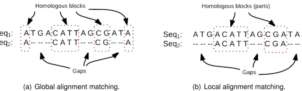
The alphabet P in above edit operations is constituted by strings (including alphabets, numbers, and/or special characters). But, in bioinformatics, it is composed by four ni-trogenous base characters when considering DNA, that is: P = {A, T , C, G}. So the pattern matching algorithms developed for strings cannot directly be applied to DNA se-quences, as both symbols and positions has biological meaning. Thus specific algorithms need to be developed by taking into account the particularity of DNA “edit operations”. For instance, deleting a part of the molecule should have approximately the same cost for small or large part, as it corresponds to only one chemical operation. Considering edit distances in the case of DNA sequences leads to two kinds of alignment algorithms: either globally align two DNA sequences as shown in Figure 3.1(a), or find the best local alignment as depicted in Figure 3.1(b).

3.2. STANDARD SUBSTITUTION MATRICES 15

(a) Global alignment matching. (b) Local alignment matching.

Figure 3.1: demonstration of sequence alignment approaches. (a) The process of global alignment. (b) The process of local alignment.

In other words, in global alignments, the entire (protein or nucleotide) sequences are aligned, while a local alignment concentrates the search on the regions of highest simi-larities within two sequences. In Figure 3.1, we can see in the two examples that DNA sequences have different sizes. It is remarkable that after applying global or local align-ment algorithm, the two sequences have the same size, which is the largest one in the global alignment case, and the size of the best common subpattern in the local one. Each column in these two sequences is called asite.Homologous sitesare columns in aligned sequences where characters are equal. For instance, in Figure 3.1(a) that represent the global alignment of sequence S1 with sequence S2, we have four homologous blocks of

eight homologous sites distributed along S1.

Gapsin both figures indicate the non-matching sites due to an insertion or deletion of k elements. The most accurate matching algorithms are those that consider an “opening gap” penalty in its scoring function, and all these alignment algorithms need to evaluate the cost of a substitution, either for nucleotides (A, T, C, G alphabet) in DNA alignment, or for amino acids (20 letters) in the protein case. This need to attribute a cost to a sub-stitution leads to the introduction of the standard subsub-stitution matrices of both nucleotides and amino acids.

3.2/

S

S

M

3.2.1/ NUCLEOTIDE SUBSTITUTION MATRICES

Codons are not uniformly distributed in the genome. Over time, mutations have intro-duced some variations in their frequency of apparition. It can be attractive to study the genetic patterns (blocs of more than one nucleotide: dinucleotides, trinucleotides...) that appear and disappear depending on mutation parameters. Mathematical models allow the prediction of such an evolution, in such a way that statistical values observed in cur-rent genomes can be recovered from hypotheses on past DNA sequences. A first model for genome evolution was proposed in 1969 by Thomas Jukes and Charles Cantor [13]. This first model is very simple, as it supposes that each nucleotide A, C, G, T has the probability m to mutate to any other nucleotide, as described in the following mutation

16 CHAPTER 3. TECHNICAL ASPECTS OF SEQUENCE ALIGNMENTS matrix,                1 − 3m m m m m 1 − 3m m m m m 1 − 3m m m m m 1 − 3m               

In this matrix, the coefficient in row 3, column 2 represents the probability that the nu-cleotide G mutates in C during the next time interval, i.e., P(G → C). This first attempt has been followed up by Motoo Kimura [14], who has reasonably considered that transi-tions (A ←→ G and T ←→ C) should not have the same mutation rate as transversions (A ←→ T , A ←→ C, T ←→ G, and C ←→ G), leading to the following mutation matrix.

               1 − a − 2b b a b b 1 − a − 2b b a a b 1 − a − 2b b b a b 1 − a − 2b               

This model was refined by Kimura in 1981 (three constant parameters, to make a distinc-tion between natural A ←→ T , C ←→ G and unnatural transversions), Joseph Felsenstein, Masami Hasegawa, Hirohisa Kishino, Taka-Aki Yano [15], and so on. Up to date mutation models encompass the General Time Reversible (GTR, [16], 1990), Tamura-Nei (TrN) in 1993 [17], or any model that describes rate variation among sites in a sequence such as gamma distribution (G) and proportion of invariable sites (I). For more information on the types of substitution matrices, reader is referred to [18].

In the next section, we will focus on amino acid substitution matrices: PAM and BLOSUM.

3.2. STANDARD SUBSTITUTION MATRICES 17

3.2.2/ POINT ACCEPTED MUTATION (PAM) MATRIX

In pairwise alignment, the Point Accepted Mutation (PAM, sometimes called Percent Ac-cepted Mutation) matrices are series of scoring matrices for amino acid1 substitution costs, each reflecting a certain level of divergence between the acids. In 1978, The researches of Margaret Dayhoff have led to the constitution of such a matrix, by just ob-serving the differences based on global alignment of closely related protein sequences with the identity score greater than 85% (see [20,21]). The first version of this matrix is called PAM1. This latter estimates of how much the rate of character substitution would

be if only 1% of amino acids residue had exchanged to another amino acid type. Dayhoff starts by calculating the relative probability ratio (mj) for each amino-acid according to the

following formula:

mj=

number of changes of j

number of occurrences of j (3.1)

The mutation probability matrix can be determined based on the following formulas: • For diagonal elements:

Mj j = 1 − λmj

where λ is a proportionality constant, and mj is the relative mutability ratio of jth

amino acid computed using Equation 3.1. • For non-diagonal elements:

Mi j=

λmjAi j

P

iAi j

where Ai jis a constant of accepted point mutation whose value can be found in [20],

λ is a proportionality constant, and mjis the relative mutability ratio of jthamino acid

computed using Equation 3.1

In further investigations, Dayhoff computed the Relatedness Odd matrix (Ri j) per amino

acid as:

Ri j =

Mi j

fi

(3.2) where, Mi j is the probability element of changing residue j to residue i in mutation

prob-ability matrix, and fi represents the frequency of residue i that may occur by chance:

fi= k

X

b

q(b)_j N(b)

where, the sum is taken over all alignment blocks b. q(b)_j is the observed frequency of amino acid j in block b, N(b) is the number of substitutions in a tree built for b and the coefficient k is chosen to ensure that the sum of the frequencies fj= 1.

The PAM1 matrix, shown in Figure 3.3(a), is at the basis of all the other PAM models like

the log-odds matrix2. Matrices such as PAM100 and PAM250 are generated to reflect the

1_{Amino-acids are inferred from different nucleotide codons, see Figure 3.2}

2_{This matrix is used by BLAST when scoring an alignment called BLOSUM (see Section 3.2.3). Indeed}

18 CHAPTER 3. TECHNICAL ASPECTS OF SEQUENCE ALIGNMENTS

different types of amino-acid substitutions that may occurred in distantly proteins, based on the hypothesis that some repeated mutations would following the similar model con-served in PAM1matrix, and multiple substitutions may occur in the related site. However,

other PAM matrices such as PAM30 and PAM70 are still used. An example of PAM250

matrix is given in Figure 3.3(b). For more information on this matrix, we recommend to read [20,21,22].

(a) PAM1matrix, all its values are scaled by 10000.

(b) A PAM250matrix. The column summation adjusted to 100.

Figure 3.3: Examples of PAM1and PAM250matrices presented in [20].

3.2.3/ BLOCKS SUBSTITUTION MATRIX (BLOSUM)

PAM matrices, introduced in the previous section, are obtained with the comparisons of closely related protein sequences, and so more divergent sequences cannot work with PAM. This is why, in 1992, Henikoff and Henikoff [23] introduced a new amino acid substitution matrix named BLOcks SUbstitution Matrix (BLOSUM). This latter is used to align protein sequences by scoring different alignments among evolutionary diverging sequences. To construct this model, a local alignment algorithm is applied on given protein sequences, then a database is scanned for highly similar block regions of protein

3.2. STANDARD SUBSTITUTION MATRICES 19

families (sequence alignment without gaps), in order to obtain the relevant frequencies of conserved amino acids with their substitution probabilities. After the exploration of amino-acids frequencies and their substitution probabilities, a computation of log-odds scores for each of the 210 possible substitution pairs of the 20 standard amino acids is applied. All BLOSUM matrices are based on observed alignments.

According to [23], BLOSUM matrices are obtained by using blocks of similar protein se-quences as input data, then various statistical approaches are applied on the data to infer similarity scores. We recalled the following pipeline steps:

• Procuring Frequency Table: In this step, a local alignment algorithm is applied on the raw data of protein sequences to infer the set of conserved blocks of fam-ilies, using an automatic tool named PROTOMAT [24], to acquire a set of scored blocks. The latter lead to construct a database of blocks. Conserved blocks are then clustered under a specific threshold to generate a set of clusters that contain a set of blocks based on identity score. In the same manner, if we want to add new sequence, then a set of matching/mismatching pairs of sequence compared with blocks should be computed. If we have a block of width w amino acids and a block depth of s sequences, it provides ws(s−1)₂ amino acid pairs. The result from this counting is a frequency table, the latter listing the number of times each of different amino acid pairs occurs among the blocks. A table is used to calculate a matrix rep-resenting the odds ratio between these observed frequencies and those expected by chance.

• Generate a Logarithm of Odds (Lod) Matrix: In this step, let the frequency table of total pairs of amino-acids be denoted by a function ( fi j). So, the function for

observed probability of each given pair is: qi j = fi j P20 i=1 Pi j=1 fi j . (3.3)

We estimate the expected probability of occurrence for each i, j pair based on it_h

amino-acids by the following formula: pi = qii+

X

j,i

qi j

2 .

The expected probability of occurrence ei j for each i, j pair is:

ei j =        pipj= p2_i if i= j, pipj+ pjpi = 2 × pipj if i , j. (3.4)

The odds ratio matrix is then calculated where each entry is qi j/ei j. A lod ratio is

then calculated in bit units as:

si j = log2(qi j/ei j)

where ei j is computed from Equation 3.4, and qi j is computed from Equation 3.3.

Lod ratios are finally multiplied by a scaling factor of 2 and then rounded to the nearest integer value to produce the BLOSUM matrix in half-bit units, as shown in Figure 3.4.

20 CHAPTER 3. TECHNICAL ASPECTS OF SEQUENCE ALIGNMENTS

Figure 3.4: The standared BLOSUM62 matrix. See [23]

Remark 1: BLOSUM Number

The number attached with BLOSUM matrix represents the identity matching score in clustering step. In other words, if the conserved blocks are clustered based on an identity score of 75%, then the generated matrix is called BLO-SUM75.

For more information on different types of BLOSUM matrix, see, e.g., [23,24]. Having the way to attribute a cost to a substitution in either DNA or protein sequences, we can now explain more deeply the alignment algorithms.

3.3/

L

A

A

In comparative biology, when we have a partial sequence of DNA and we need to pro-vide some information about it, the first idea is to compare this sub-sequence (pattern) with a database of already identified sequences, seeking for relatively conserved sub-sequences [25] using local alignment algorithms (LSA). This process will find the con-served regions of this partial sequence in the database, providing thus information thanks to the reference sequence.

There are many algorithms developed for this kind of alignment. In next sub-sections, we will summarize some of the most popular ones.

3.3.1/ BASIC LOCAL ALIGNMENT SEARCH TOOL (BLAST)

In 1985, David J. Lipman and William R. Pearson [26] have developed a software pack-age for protein-protein sequence similarity search called FASTP for proteins and FASTN for nucleotides. These software have been popularized under the name of FASTA, which is an abbreviation of “FAST-All”. This tool combines the ability to do DNA-DNA and trans-lated protein-DNA searches.The FASTA file format is now widely used by other sequence

3.3. LOCAL ALIGNMENT ALGORITHMS 21

database search tools, such as BLAST Altschul [25], and sequence alignment programs like ClustalW [27], MUSCLE [28], T-COFFEE [29], etc.

In 1990, a more time-efficient algorithm than FASTA, called Basic local alignment search tool (BLAST), was developed by Altschul [25]. BLAST is a heuristic algorithm that gives a comparison approximation of the best local alignment between biological amino-acid sequences of protein, or nitrogen base sequences. It enables bioinformatic researchers to compare a desired query sequence with a library of sequence databases, in order to identify the target sequences that are the most similar with the desired query (given a certain threshold). Having the same sensitivity than FASTA, BLAST is more reliable as it only searches the most significant patterns in the sequence database. Note that various versions of BLAST have been developed by the National Center of Biotechnology Information NCBI.

There are various software versions of BLAST depending on the type of the queried sequence:

• BLASTN: Program that searches in nucleotide databases using a nucleotide query. • BLASTP: Program that investigates protein databases using a protein query. • BLASTX : Search in protein databases using a translated nucleotide query (e.g.,

protein query).

• TBLASTN: Search in translated nucleotide databases using a protein query. • TBLASTX : Search in translated nucleotide databases using a translated nucleotide

query.

3.3.2/ SMITH–WATERMAN ALGORITHM

The Smith-Waterman is an algorithm based on dynamic programming developed by Smith in 1981. Its main purpose is to align locally two biological sequences in order to discover in minimal cost the optimal alignment path [30]. It is independent of any distance function (such as Euclidean, Manhattan, or Levenshtein that will be detailed in Section 3.5). The algorithm calculates the alignment that minimizes the costs provided by a certain distance function. It aims to align two sequences in a way that similar sub-sequences are aligned together. Local alignment is very useful when we want to align a partial portion of a sequence with a database of biological sequences. It can be applied in computer science in many applications, especially with those that need database search (such as data mining, information retrieval, pattern matching, image processing, etc.). In this algorithm, a two dimensional scoring matrix T of size (m+1)×(n+1) is formed from the two provided biological sequences3of length n and m. One extra column and one row containing zeros are added to the matrix, for score computation. The score in each cell is computed based on the scoring function presented in Equation 3.5.

Remark 2: Zero state inSWmatrix

If the scoring numbers generated from the first three rules in Equation 3.5 are negative, then zero must be inserted in the cell T (i, j) to ensure to have no neg-ative value in the matrix.

22 CHAPTER 3. TECHNICAL ASPECTS OF SEQUENCE ALIGNMENTS T(i, j)= max                    T(i − 1, j − 1)+ σ(ai, bj),

T(i, j − 1) − gap penalty, T(i − 1, j) − gap penalty, 0.

(3.5)

where T (i, j) is the value at line i and column j of the scoring matrix of aiand bj. The value

σ(ai, bj) is provided by a standard substitution matrix, like those detailed in Section 3.2

Note that some parameters can be optionally specified for the match, mismatch, and gap penalties in the scoring matrix.

Let us now consider that we have two nucleotide sequences A and B of different sizes, where A= a1a2a3...an and B= b1b2b3...bm, and let us explain how to compute the scoring

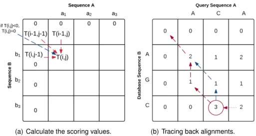
matrix T . Figure 3.5(a) shows that SW uses an individual pairwise comparisons between characters to fill the scoring matrix. In this figure, to compute the value of T (i, j), we need to take into consideration all the four scoring options and select the maximum one. When the matrix T is all computed, a new process starts by tracing back the matrix by selecting the position of maximum score. Then, from that position, we go up following the maximum score until reaching the first diagonal position. The selected positions in trace back process is considered as the optimal alignment path, as shown in Figure 3.5(b).

(a) Calculate the scoring values. (b) Tracing back alignments.

Figure 3.5: Example of Smith-Waterman local alignment algorithm of two given se-quences (A, B), A = a1a2a3...an and B = b1b2b3...bm. (a) Calculate a new matching score

depending heuristically on the previous around values. (b) Tracing back the alignment by starting from the maximum score in the generated matrix, then follow the maximum score on each step up.

3.4. GLOBAL SEQUENCE ALIGNMENT: THE NEEDLEMAN WUNSCH EXAMPLE 23

3.4/

G

S

A

:

N

W

In global alignments, we compare the entire sequences by counting the amount of identi-cal residues along the alignment. We explain in what follows how one of these algorithms works, namely the Needleman Wunsch algorithm.

The Needleman–Wunsch algorithm has been firstly developed by Saul B. Needleman and Christian D. Wunsch in 1970 [NW70]. This algorithm follows the concepts of dynamic programming: it divides a large problem (e.g., the full sequence) in a series of smaller ones more tractable. Then, it solves the smaller problems in order to finally provide a solution for the larger one. The Needleman-Wunsch algorithm is still widely applied for optimal global alignment, especially when the quality of the global alignment is of high importance.

This algorithm is constituted by the following steps:

• Setting up the matrix: let A= a1a2a3. . . anand B= b1b2b3. . . bmbe two sequences

of different sizes that we want to compare. A two-dimensional matrix T should be computed. In this matrix, the row vector represents sequence A while the column one corresponds to sequence B. A perfect correspondence or a mismatch align-ment between these two sequences is represented by a diagonal line as shown in Figure 3.6(a). A gap in the first sequence leads to a horizontal line (Figure 3.6(b)), while a gap in the second sequence is drawn as a vertical line, as shown in Fig-ure 3.6(c).

(a) Identical sequence match-ing.

(b) Gaps in horizontal lines. (c) Gaps in vertical lines.

Figure 3.6: Example of Needleman Wunsch global alignment algorithm of two given se-quences A= a1a2a3...anand B= b1b2b3...bm. (a) A diagonal line is when the two characters

are equal, or when there is a substitution of characters. (b) Gaps in the first sequence are expressed from horizontal line. (c) Gaps in the second sequence correspond to vertical lines.

• Scoring the Matrix: In Needleman-Wunsch algorithm, we fill the matrix T in the same manner than in Smith-Waterman, as shown in Figure 3.7(b):

24 CHAPTER 3. TECHNICAL ASPECTS OF SEQUENCE ALIGNMENTS T(i, j)= max              T(i − 1, j − 1)+ σ(ai, bj) T(i − 1, j) − gap penalty T(i, j − 1) − gap penalty

(3.6)

Remark 3: Needleman-Wunsch vs Smith-Waterman

The main differences between Needleman-Wunsch and Smith-Waterman algorithms are:

– The zero condition: in SW algorithm, we insert a 0 in the cell i, j if Ti, j

is negative, which is not the case in the NW one.

– Sequences in scoring matrix are ordered in an opposite direction.

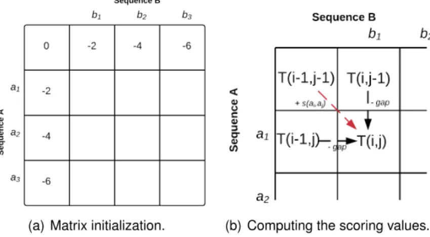
A computation example of scoring matrix is given in Figure 3.7.

(a) Matrix initialization. (b) Computing the scoring values.

Figure 3.7: Example of Needleman-Wunsch global alignment algorithm of two given se-quences A = a1a2a3...an and B = b1b2b3...bm. (a) The initialization of the scoring matrix.

(b) How to calculate the next score: (+1) for matching, (-2) for mismatching, and (-2) for gap penalty.

• Identify the optimal path: In Figure 3.8, the tracing back process starts from the lowest right position in the scoring matrix, following the maximum scores until reaching the upper left position. The path drawn by this matrix is considered as the optimal alignment path given for aligning the two sequences.

3.5/

E

In computer science and information retrieval, edit distance is a way of clarifying how different two strings are. This latter can be achieved by counting the minimum number of events that are required to convert one word into another one. Edit distances are used in various application domains, for example in natural language processing where the automatic spell corrections are determined according to the closest word in a given

3.6. MULTIPLE SEQUENCE ALIGNMENT (MSA) 25

Figure 3.8: Tracing back the alignment by starting from the lowest right corner and follow-ing the maximum score on each step up.

dictionary. In bioinformatics, such distances are used to evaluate the similarity of DNA or amino acid strings.

Needleman-Wunsch alignment algorithm can be used to provide an edit distance with gaps, as the lowest right column of the scoring matrix contains the scoring cost. If the distinction between gap opening and extension is not required, and if we only need to consider insertion, deletion, and substitution of characters, then the Levenshtein edit dis-tance can be used. This latter corresponds to usual spelling errors like in gene names, while the former is more adequate when considering usual chemical modifications of biomolecules (this fact will be used in our first contribution). Let us bring more details about the Levenshtein distance.

The string metric proposed by Vladimir Levenshtein in 1965 [32,33], is defined formally as the minimum number of insertion, deletion, or substitution operations required to change one word into the other one. Mathematically speaking, the Levenshtein distance between A, a string of length n, and B, another string of length m, can be computed using the same dynamic programing canvas than in Needleman-Wunch, except that T matrix is filled as follows: T(i, j)=                   

max (i,j) if min (i,j)= 0,

min              T(i − 1, j)+ 1 T(i, j − 1)+ 1 T(i − 1, j − 1)+ 1(ai,bj) Otherwise. where 1(ai,bj) is 1 if and only if ai, bj and 0 otherwise.

3.6/

M

S

A

(MSA)

Dynamic programming as described by Needleman-Wunsch for pairwise alignment is guaranteed to identify the optimal global alignment. Exact methods for multiple sequence alignment employ dynamic programming too.

The goal here is to maximize the summed alignment score of each pair of sequences. Exact methods generate optimal alignments but are not feasible in time or space for more than a few sequences. MSA are easy to generate for a group of very closely related protein (or DNA) sequences, as shown in Figure 3.9, as soon as the sequences exhibit

26 CHAPTER 3. TECHNICAL ASPECTS OF SEQUENCE ALIGNMENTS

some divergence, the problem of multiple alignment becomes extraordinary difficult to solve. The Multiple Sequence Alignment (MSA), is a collection of three or more nucleic acid (or protein) sequences that are partially or completely aligned. Homologous residues are aligned in columns across the length of the sequences. These aligned residues are homologous in a structural sense or even in an evolutionary sense: they are presumably derived from a common ancestor.

Figure 3.9: Multiple sequence alignment editing of different sequences of Apiales order. The MUltiple Sequence Comparison by Log-Expectation (MUSCLE) measures the dis-tance between given sequences by iteratively refining multiple sequence alignment by deleting the edge of the guide trees to form a bi-partition, and then extracting pair of pro-files and realigning then. Several functions are applied to align pairs of columns optimally. MUSCLE uses the sum-of-pairs (PSP) profile in the scoring function:

PSPxy=X

i

X

j

f_ixf_jySi j

where PSPxy is a sequence-weighted sum of substitution matrix scores for each pair of latters. Si j is the log expectation Si j = log(pi j/pipj). MUSCLE applies two PAM matrices

and new log-expectation score for its PSP function: LExy= (1 − f_Gx)(1 − f_Gy)logX i X j f_ixf_jy pi j pipj

where the factor (1 − fG) is the occupancy of a column. For more information, see [28].

3.7/

C

In this chapter, we recall various algorithms of sequence alignments based on computing the edit distance. Computing the edit distance means that we considered the minimum edit operations that change one sequence into other one. In bioinformatics, sequence alignment algorithms lie in two types: local and global alignment algorithms.

In local alignment algorithms, a query sequence is aligned with a database of well-known protein or nucleotide sequences, where there are some regions with highest similarity score. Well-known algorithms for Local alignment are BLAST and Smith-Waterman. For global alignment, two sequences are aligned based on the computation of optimal align-ment path. This latter is computed from a scoring function by tracing back the scoring matrix from the lower right cell following the maximum scores until reaching the upper left cell. Distance measures such as Levenshtein, Euclidean, and Manhattan distances are also detailed. Levenshtein measure is not an alignment algorithm, but it takes into account some edit operations such as insertion and deletion.

Finally, we detailed MUSCLE algorithm of multiple sequence alignment tools. We ex-plained that this algorithm use the sum-of-pairs (PSP) profile with two PAM matrices and novel log-expectation formula.