HAL Id: tel-01893462
https://tel.archives-ouvertes.fr/tel-01893462
Submitted on 11 Oct 2018
HAL is a multi-disciplinary open access
archive for the deposit and dissemination of sci-entific research documents, whether they are pub-lished or not. The documents may come from teaching and research institutions in France or abroad, or from public or private research centers.
L’archive ouverte pluridisciplinaire HAL, est destinée au dépôt et à la diffusion de documents scientifiques de niveau recherche, publiés ou non, émanant des établissements d’enseignement et de recherche français ou étrangers, des laboratoires publics ou privés.
detectors duty cycle by reduction of parametric
instabilities and environmental impacts
Sébastien Biscans
To cite this version:
Sébastien Biscans. Optimization of the Advanced LIGO gravitational-wave detectors duty cycle by reduction of parametric instabilities and environmental impacts. Mechanics of materials [physics.class-ph]. Université du Maine, 2018. English. �NNT : 2018LEMA1019�. �tel-01893462�
T
H
ÈSE DE DOCTORAT DE
LE MANS UNIVERSITÉ
COMUE UNIVERSITÉ BRETAGNE LOIRE
ÉCOLE DOCTORALE No602 Sciences pour l'Ingénieur
Spécialité : Mécanique des Solides, des Matériaux, des
structures et des surfaces
Par
Sébastien BISCANS
Optimization of the Advanced LIGO gravitational-wave detectors duty
cycle by reduction of parametric instabilities and environmental impacts
Optimisation du cycle de service de l’observatoire d’ondes gravitationnelles LIGO
par réduction des instabilités paramétriques et des impacts environnementaux
Rapporteurs avant soutenance :
Christophe COLLETTE, Professeur étranger, Université libre de Bruxelles, Bruxelles Emmanuel FOLTÊTE, Professeur des Universités, FEMTO-ST, Besancon
Composition du Jury :
Président :
Matteo BARSUGLIA, Directeur de Recherche CNRS, Université Paris Diderot – Astroparticule et Cosmologie, Paris
Examinateurs :
Simon CHESNE, Maître de conférences, INSA Lyon, Villeurbanne Cécile Guianvarc’h, Maître de conférences, CNAM, Paris
Dir. de thèse :
Charles PEZERAT, Professeur des Universités, Université du Maine, Le Mans
Co-dir. de thèse :
Pascal PICART, Professeur des Universités, Université du Maine, Le Mans
Co-encadrant de thèse :
Matthew EVANS, Professeur étranger, Massachusetts Institute of Technology, Cambridge
Invité :
Thèse présentée et soutenue au Mans, le 21 septembre 2018
Unité de recherche: Laboratoire d’Acoustique de l’Université du Maine ─ UMR CNRS 6613 Thèse N°: 2018LEMA1019
Optimization of the Advanced LIGO gravitational-wave detectors duty cycle by reduction of parametric instabilities and environmental impacts
Keywords: gravitational-wave, seismic isolation, earthquake, controls, parametric instability, materials, mechanics, optics.
Abstract
The LIGO project (Laser Interferometer Gravitational-Wave Observatory) is a large-scale physics experiment the goal of which is to detect and study gravitational waves of astrophysical origin. It is composed of two instruments identical in design, one located in Hanford, WA and the other in Livingston, LA in the United States. The two instruments are specialized versions of a Michelson interferometer with 4km-long arms. They observed a gravitational-wave signal for the first time in September 2015 from the merger of two stellar-mass black holes. This is the first direct detection of a gravitational wave and the first direct observation of a binary black hole merger. Five more detections from binary black hole mergers and neutron stars merger have been reported to date, marking the beginning of a new era in astrophysics. As a result of these detections, many activities within the LIGO collaboration are in progress to improve the duty cycle and sensitivity of the detectors. This thesis has been conducted at the Massachusetts Institute of Technology (MA, USA), as part of the LIGO Research & Development activities. It addresses two major issues limiting the duty cycle of the LIGO detectors: environmental impacts, especially earthquakes, and the issue of unstable opto-mechanical couplings in the cavities, referred to as parametric instabilities.
Earthquakes
LIGO requires an unprecedented level of isolation from the ground. When in opera-tion, the interferometers are expected to measure motion of less than 10−19 meters. Strong teleseismic events like earthquakes disrupt the operation of the detectors, and result in a loss of data until the detectors can be returned to their operating states. A variety of seismic control strategies have been studied to reduce the downtime due to earthquakes. Early results have shown a downtime reduction of ∼ 40% at one of the LIGO sites, thus suggesting that this strategy can significantly reduce the impact of earthquakes on the LIGO detectors. Other strategies have also shown promising results but will have to be tested in the future. We present a plan to implement these new earthquake configurations in the LIGO automation system.
Parametric instabilities
A parametric instability results from an opto-mechanical coupling between the me-chanical modes of a mirror and the optical modes of the cavity. In the case of the LIGO interferometers, the large amount of stored optical power and high
mechani-and sensitivities. To reduce these instabilities, an electro-mechanical device, called ’Acoustic Mode Damper’ (AMD), has been designed and tested to damp the me-chanical modes associated with parametric instabilities. Measurements have shown a significant reduction in the quality factor of several mechanical modes in accor-dance with our model. This suggests that AMDs should solve the issue of parametric instabilities for LIGO.
In conclusion, we will show that the issues tackled in this thesis improved the overall duty cycle of LIGO by 4.6%, which corresponds to an increase of the gravitational-wave detection rate by 14%.
Optimisation du cycle de service de l’observatoire d’ondes
gravitationnelles LIGO par r´eduction des instabilit´es param´etriques et des impacts environnementaux.
Mots cl´es: onde gravitationnelle, isolation sismique, tremblement de terre, contrˆole, instabilit´e param´etrique, mat´eriau, m´ecanique, optique.
R´esum´e
Le projet LIGO (pour Laser Interferometer Gravitational-Wave Observatory) a pour but la d´etection et l’´etude d’ondes gravitationnelles via un r´eseau de d´etecteurs. LIGO poss`ede deux d´etecteurs d’architecture et de fonctionnement identiques, l’un situ´e dans l’´Etat de Washington et l’autre dans l’´Etat de Louisiane aux ´Etats-Unis. Chaque d´etecteur est une version consid´erablement am´elior´ee d’un interf´erom`etre de Michelson avec des bras optiques de 4 km de long. Ces interf´erom`etres ont observ´es le signal ´emis par un trou noir binaire sous la forme d’une onde gravitationnelle pour la premi`ere fois en septembre 2015. Depuis, cinq autres d´etections ont ´et´e r´ealis´ees par les observatoires de LIGO. Ces d´etections marquent le d´ebut d’une nouvelle `ere pour l’astrophysique, en liaison ´etroite avec la physique des trous noirs et des ´etoiles `
a neutrons.
Malgr´e ces d´etections, un grand nombre d’activit´es de la collaboration scientifique de LIGO sont en d´eveloppement pour perfectionner les interf´erom`etres. Cette th`ese s’est deroul´ee au Massachusetts Institute of Technology (MA, USA), et s’inscrit dans le cadre du programme de recherche et d´eveloppement du laboratoire LIGO. Elle a pour objectif d’am´eliorer le temps de service des d´etecteurs, en r´epondant en parti-culier `a deux probl´ematiques majeures: le probl`eme des impacts environnementaux, et notamment celui des tremblements de terre, ainsi que le probl`eme des instabilit´es param´etriques.
Tremblements de terre
LIGO requiert des besoins sans pr´ec´edent en termes d’isolation sismique. Chaque in-terf´erom`etre doit ˆetre capable de mesurer un mouvement de l’ordre de 10−19 m`etres. L’importante amplification de l’activit´e sismique g´en´er´ee par certains tremblements de terre peut ainsi empˆecher l’interf´erom`etre de fonctionner correctement. Plusieurs strat´egies de contrˆole actif ont ´et´e ´etudi´ees pour r´eduire les p´eriodes d’instabilit´es du-rant de tels ´ev´enements. Les r´esultats pr´emilinaires montrent une r´eduction du temps d’arrˆet g´en´er´e par les tremblements de terre d’environ 40% `a un des observatoires. D’autres strat´egies ont ´et´e d´evelopp´ees et seront test´ees dans le futur. Un plan pour utiliser ces strat´egies via le syst`eme d’automation de LIGO est pr´esent´e.
Une instabilit´e param´etrique provient d’un couplage opto-m´ecanique entre le mode m´ecanique d’un mirroir et un ou plusieurs mode(s) de cavit´e. Dans le cas des in-terf´erom`etres de LIGO qui op`erent `a haute puissance, ce couplage peut devenir rapi-dement instable. Ces instabilit´es empˆechent les interf´erom`etres de fonctionner cor-rectement, limitant leur cycle de service et sensibilit´e. Pour pallier `a ce probl`eme, un amortisseur ´electrom´ecanique, appel´e ’Acoustic Mode Damper’ (AMD) a ´et´e concu et developp´e. Il permet de consid´erablement r´eduire le facteur de qualit´e des modes m´ecaniques probl´ematiques, et par-del`a mˆeme les instabilit´es. D’apr`es le mod`ele et les premi`eres mesures, les AMDs devraient compl`etement r´esoudre le probl`eme des instabilit´es param´etriques pour LIGO.
En conclusion, il sera demontr´e en quoi les probl´ematiques r´esolues pendant ce travail de th`ese ont permises d’am´eliorer le cycle de service des d´etecteurs de LIGO de 4.6%, ce qui correspond `a une augmentation du nombre d’ondes gravitationnelles detect´ees par an de 14%.
Acknowledgements
Over the years, before and during my thesis, LIGO has always been a fascinating, engaging challenge. It has been a singular privilege to interact and work with the numerous scientists of the LIGO Scientific Collaboration. This is a very long list of people, and it is not possible to name them all. However, I would be remiss not to draw attention to a certain number of people.
First, I would like to express my gratitude and appreciation to Dr Christophe Collette and Dr Emmanuel Foltˆete for reviewing this work as rapporteurs. My thanks also go to Dr Matteo Barsuglia, Dr Simon Chesne, Dr C´ecile Guianvarc’h and Dr David Shoemaker for being part of this committee.
My supervisors in France, Charles Pezerat and Pascal Picart, deserve special thanks as well. Despite me being on the other side of the world, Charles and Pascal always seemed to know what I was doing better than I did. Without their knowledge, insight and guidance I’d never have made it this far.
Same goes to my supervisor at MIT, Matthew Evans, who is one of the most knowl-edgeable person I know. His guidance and vision on a project like LIGO has shaped what makes me a scientist today. Thank you Matt especially for your patience and the time you took for me.
Next, I have to give a special shout-out to the brilliant Slawek Gras, with whom I worked many (too many) hours in the lab on the AMD project. Thank you Slawek for the extra-hours you took for me, for your guidance, your advice, and the many coffees and beers. A-team forever.
Special thanks also to Richard Mittleman for putting up with me over all those years. Don’t worry Rich, I still have a lot of stupid questions for you.
Thanks to Peter Fritschel for supporting me and giving me a fascinating project to work on. Thanks to Myron for all the help downstairs, could not have done it without you. Thanks to Betsy and Travis for the help and laughs in chamber and on the bocce court. Thanks to the Livingston team for making sure I always have a good time on site. Thanks to Rainer Weiss for this crazy project.
Lastly, to the loved ones in my life. To my mum, dad and sister, without you I wouldn’t be where I am now. Thank you for your patience, love and for always believing in me.
Contents
1 Introduction 33 1.1 Gravitational radiation . . . 33 1.2 Sources . . . 34 1.2.1 Binary inspirals . . . 35 1.2.2 Supernovae bursts . . . 35 1.2.3 Continuous waves . . . 36 1.2.4 Stochastic background . . . 361.3 Interferometric gravitational-wave detectors . . . 36
1.3.1 Michelson . . . 36
1.3.2 Fabry-Perot arm cavities . . . 37
1.3.3 Power and signal recycling . . . 37
1.4 Detectors around the world . . . 38
2 LIGO 41 2.1 Introduction . . . 41
2.2 Detections . . . 42
2.2.2 GW151226 . . . 43
2.2.3 GW170104 . . . 43
2.2.4 GW170608 . . . 44
2.2.5 GW170814 . . . 45
2.2.6 GW170817 . . . 45
2.3 The LIGO interferometer . . . 47
2.4 Noise . . . 48
2.4.1 Seismic noise . . . 48
2.4.2 Gravity gradient noise . . . 49
2.4.3 Suspension and coating thermal noise . . . 50
2.4.4 Residual gas noise . . . 52
2.4.5 Quantum noise . . . 52
2.5 Current limitations for Advanced LIGO . . . 54
2.5.1 Sensitivity . . . 54
2.5.2 Duty cycle . . . 55
2.6 Objective of this thesis . . . 56
3 Environmental impacts on large-scale interferometers: study of earth-quakes 57 3.1 The problematic . . . 57
3.2 Introduction to earthquakes . . . 58
3.3 Seismon . . . 59
3.3.1 Description . . . 60
CONTENTS
3.3.3 Velocity prediction . . . 61
3.3.4 Threat prediction . . . 62
3.3.5 Output . . . 66
3.4 Ground behavior at the sites . . . 68
3.4.1 Local motion . . . 68
3.4.2 Common motion . . . 69
3.5 Control strategies . . . 70
3.5.1 Seismic platform architecture . . . 70
3.5.2 Seismic control scheme . . . 72
3.5.3 Tilt-Horizontal coupling . . . 76
3.5.4 O1 nominal configuration and performance . . . 78
3.5.5 First strategy: Tilt reduction. . . 80
3.5.6 Second strategy: Gain peaking reduction . . . 84
3.5.7 Third strategy: Common mode rejection along the arms . . . 87
3.6 Implementation at the sites . . . 93
3.7 Conclusion . . . 93
4 Parametric Instabilities 96 4.1 Background . . . 96
4.1.1 Introduction to PI . . . 96
4.1.2 Calculation of the parametric gain . . . 97
4.1.3 Overlap parameter Bm,n calculation . . . 102
4.2 PI model & prediction . . . 111
4.2.1 Mechanical mode calculation (nominal values) . . . 111
4.2.2 Model . . . 113
4.3 Current status of LIGO . . . 115
4.4 Damping solution: Acoustic Mode Damper . . . 117
4.4.1 Description . . . 117
4.4.2 Shunted piezoelectric . . . 118
4.4.3 AMD material selection . . . 124
4.5 Experiment . . . 127
4.5.1 Approach . . . 128
4.5.2 Limitations and preliminary results . . . 129
4.5.3 Final design . . . 132
4.6 Epoxy bulk loss factor . . . 134
4.7 Epoxy thin layer loss . . . 135
4.8 Piezoelectric results . . . 138
4.9 AMD model . . . 140
4.9.1 AMDs designs . . . 141
4.9.2 Location . . . 142
4.9.3 Performance against PI . . . 144
4.9.4 AMD thermal noise . . . 147
4.10 Installation . . . 150
4.10.1 AMD assembly . . . 150
CONTENTS
4.11 Results . . . 159
4.11.1 AMDs performance . . . 159
4.11.2 AMDs thermal noise . . . 161
4.12 Conclusion . . . 162
A Logistic cost function simplification 166 B Radiation pressure calculation 168 C Relationship between HOM field and sideband field 170 D Calculation of the resistive shunt mechanical impedance 171 E PZT materials tested 172 F Thermoelastic effect 173 G Tuning of the mechanical oscillator 175 G.1 Tuning of the oscillator . . . 175
G.2 Tuning of the suspension . . . 176
G.2.1 Application . . . 179
H FEA analysis 180
List of Figures
1.1 Evolution with time of a + and × polarized GWs, propagating into
the page. . . 34
1.2 Isometric view of a GW at a given instant. Propagation along the tube (Numerical simulation. Credits: einstein-online.info). . . 35
1.3 IFO response to the + polarized gravitational wave from figure 1.1. The test masses of the IFO behave as free masses and therefore are sensitive to strain. When the IFO is deformed, we observe light inten-sity modulations at the output photodetector (in green). . . 37
1.4 Overview of a Michelson IFO coupled with Fabry-Perot cavities in the arms. It is composed by an input laser, a beam-splitter (BS), two input mirrors (ITM), two output mirrors (ETM) and an output photodetector. The suffixes X and Y denote the two different arms in the x and y direction respectively. . . 38
1.5 Overview of a Fabry-Perot Michelson IFO, coupled with a power recy-cling cavity at the input, and a signal recyrecy-cling cavity at the output. 39 1.6 Overview of the international network of ground-based GW detectors. 39 2.1 Location and orientation of the LIGO detectors at Hanford, WA (H1) and Livingston, LA (L1). . . 42
2.2 GW150914 event . . . 43
2.3 GW151226 event . . . 43
2.4 GW170104 event . . . 44
2.6 GW170814 event . . . 45 2.7 GW170817 event . . . 46 2.8 Layout of the Advanced LIGO detector. . . 47 2.9 Estimation of the seismic noise in the LIGO detection bandwidth. . . 49 2.10 Estimation of the Newtonian noise in the LIGO detection bandwidth.
The change of slope around 10Hz is due to the different sources of noise. Below 10Hz, the noise is mostly generated by seismic waves (seismic gravity gradient noise), while above 10Hz, it is created by atmospheric disturbances (atmospheric gravity gradient noise). . . 50 2.11 Estimation of the thermal noise. The noise associated with the fibers
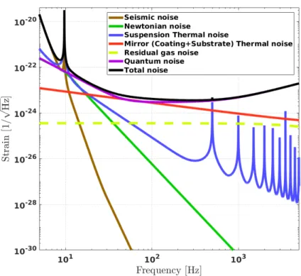
is plotted in blue. The several high-frequency peaks correspond to the different violin modes and harmonics of the fibers. The noise associated with the mirrors is shown in red (it is grandly due to the coating). . . 51 2.12 Estimation of the excess gas noise. . . 52 2.13 Estimation of the quantum noise (in purple). All the strain noise are
added in quadrature to calculate the total noise of Advanced LIGO at full power. . . 54 2.14 Strain sensitivity comparison between Advanced LIGO at Hanford
(H1) and Livingston (L1) during O1 and the designed sensitivity for Advanced LIGO (same curve that the one presented in figure 2.13). . 55 2.15 Advanced LIGO duty cycle distribution during the O1 period, from
September 2015 to January 2016. . . 56
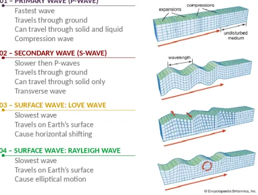
3.1 Summary of the different seismic waves generated by an earthquake. They are listed from the fastest to the slowest. . . 59 3.2 A flowchart of the Seismon pipeline. USGS information is used to
estimate time arrivals, peak ground velocity and threat level for the IFO. 60 3.3 PREM velocity model . . . 61 3.4 Seismon velocity prediction . . . 62 3.5 Standard logistic function h(x). Note that h(x) ∈ {0, 1} for all x. . . 64
LIST OF FIGURES
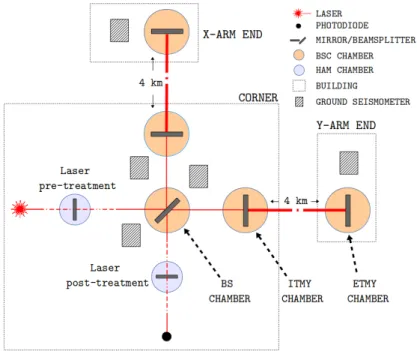
3.6 Performance of the logistic regression classifier at Hanford and Liv-ingston. True positive rate is the ratio of the sum of predicted positive condition actually being true to the sum of all actually positive con-ditions. Positive condition here refers to a lockloss prediction by the classifier which in general can be true or false. False positive rate is the ratio of the sum of predicted positive condition being false to the sum of all actually negative conditions. Classifier prediction about the detector being in lock forms the negative condition. The area under the curves assesses the efficiency of this classifier. . . 65 3.7 Seismon gaphical interfaces . . . 67 3.8 Simplified optical layout of the LIGO detector, showing the
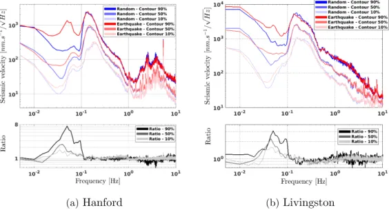
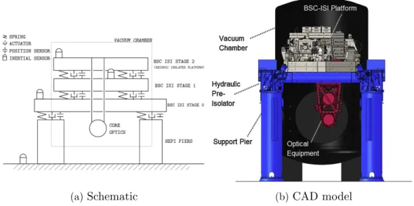
approx-imate positions of the ground seismometers at the sites. For clarity, Laser pre-treatment and Laser post-treatment regroup all of non-core optics and the multiple vacuum chambers in which they are housed. . 68 3.9 Ground spectra at the sites . . . 69 3.10 Comparison between the common and differential motions in the
cor-ner station and along the Y-arm at both sites. Data were selected at random times (blue curves), and during earthquakes of Richter mag-nitude 5 or greater (red curves). In the corner station at Livingston, we see a ratio of 90% between 100mHz and 1Hz instead of 100%. We believe this is due to a calibration issue between the seismometers. . . 71 3.11 Overview of the BSC chamber . . . 72 3.12 Control block diagram of a seismic isolation stage for one degree of
freedom. The colored blocks are related to figure 3.13. . . 73 3.13 Example of the LIGO seismic control scheme performance on the
BSC-ISI stage 1 platform. The dashed curves show the different filters used, as opposed to the solid curves showing the transfer functions from the ground motion with different loops engaged. . . 75 3.14 Model considered to estimate the tilt coupling in horizontal seismometers. 76 3.15 A more realistic control block diagram for one degree of freedom,
in-cluding the tilt seen by the seismometers. The only difference between the translational degree of freedom Y and the rotational degree of free-dom RX is that rotation has the feedback loop engaged only (no sensor correction nor feedforward), since there is no rotation sensors on the ground. . . 78
3.16 Simulink model for the BSC-ISI stage 1 platform. . . 79 3.17 Seismic isolation provided by BSC-ISI stage 1 in the Y-direction at
both sites. The black curve represents a typical ground motion, and the blue curve the measured motion of the stage. The dotted curve in-dicates the LIGO goal to obtain from 200mHz to higher frequencies for stage 1. The thinner curves indicate the estimated noise contributions, and the red curve shows the simulated overall motion. . . 80 3.18 Comparison between the common and differential motion in the corner
station and along the Y-arm at both sites. Data were selected at ran-dom times (blue curves), and during earthquakes of Richter magnitude 5 or greater (red curves). . . 81 3.19 Comparison of the filters used during O1 (dashed lines) and the new
designed filters for earthquakes (solid lines). The left part of the figure shows the complementary low-pass and high-pass filters. The right part shows the sensor correction filters. . . 82 3.20 Seismic isolation provided by BSC-ISI stage 1 in the Y-direction at
both sites. The black curve represents a typical ground motion, and the blue curve the measured motion of the stage during O1 and the red curve the predicted stage motion with the new filters. The thinner curves indicate the estimated noise contributions with these new filters. 83 3.21 Comparison of the interferometer behavior between O1 and O2 at
Han-ford. The figure shows the IFO status versus the peak ground velocity in the [30mHz-100mHz] band, with the blue bars for when the IFO stayed lock and the yellow bars for when the IFO lost lock. The y-axis represents the percentage of events per bin, with the number above each bar being the total number of events per bin. . . 84 3.22 Comparison of stage 1 ITM behavior in the [30mHz-100mHz] band
for different ground motions: stretches selected during earthquakes when the interferometer survived(blue curve), stretches selected dur-ing earthquakes when the interferometer stops functiondur-ing (red curve). The top part of the figure represents the cumulative distribution func-tion for the ground and the stage respectively, as a funcfunc-tion of the peak velocity for each stretch. The plots indicate the direct correlation be-tween velocity and the interferometer status at both sites. We observe a net increase of the stage velocity compared to the ground, due to self-inflicted gain peaking in this frequency band. The bottom part of the plots represents P (LL|v), the smoothed probability of losing lock as a function of peak velocity. It is computed by fitting the measured probability with a hyperbolic tangent function. . . 85
LIST OF FIGURES
3.23 Comparison of the filters used during O1 (dashed lines) and the new designed filters for earthquakes (solid lines). The left part of the figure shows the complementary low-pass and high-pass filters. The right part shows the sensor correction filters. . . 86 3.24 Seismic isolation provided by BSC-ISI stage 1 in the Y-direction at
both sites. The black curve represents a typical ground motion, and the blue curve the measured motion of the stage during O1 and the red curve the predicted stage motion with the new filters. The thinner curves indicate the estimated noise contributions with these new filters. 86 3.25 New P(vnew) distribution based on O1 data with P(vnew) = P(v)1.5 . As a
reminder from figure 3.22, we plotted the probability of losing lock as a function of stage velocity P(LL|v) in black. . . 87 3.26 Overview of the implementation necessary to control only on local
dif-ferential motion at low frequency during earthquakes. . . 88 3.27 Control scheme of the new configuration. To obtain the local
differen-tial motion of ITMY, the local ground YG0 from ETMY is subtracted from the local ground YG. The difference (YG− YG0) is then multiply
by 0.5 and added to the sensor correction path. Nin0 and Stilt0 represent the noise and tilt associated with the ETMY ground seismometer. . . 89 3.28 Simulink models developed for the presented strategy. In the first
model, the differential motion is added as an additional input. In the second model, both ITMY and ETMY platforms are simulated. In this model, tilt, noise and feedforward are not considered. . . 90 3.29 Time-series of the seismometers close to the Hanford ITMY chamber
(blue curve) and the ETMY chamber (orange curve) during a Richter magnitude 6.5 in Alaska. We clearly see the first arrival of the P-waves around 300s. A vertical offset was put on the two curves for visibility. The differential signal is in yellow. This data is used in the Simulink models presented in this section. . . 91
3.30 Left figure: Comparison of performance between the nominal configu-ration and the new configuconfigu-ration described in this section. The orange and red curves are simulated using the frequency domain Simulink model shown in figure 3.28. We observe a disparity between the mea-sured and simulated performance for the nominal configuration above 500mHz (blue and orange curves). This is due to the simple plant model used in the simulation, as explained before. The new configura-tion degrades the performance above 500mHz and improves it around 50mHz. Right figure: Time-series (generated with the time domain Simulink model) of the Y drive signal (as a velocity) of the nominal and new configuration. We observe a reduction of the peak velocity by ∼ 25% . . . 92 3.31 State graph of the BSC-ISI Guardian system. The ovals represent the
different states, and the arrows the authorized transitions from one state to another. Eight different states are needed to fully isolated a BSC chamber to a nominal configuration. Represented in orange is the new states necessary to have the earthquake configuration part of the automation system. The solid arrows show the path to go from nominal to Earthquake configuration, and the dash arrows the path from Earthquake to nominal. . . 94
4.1 PI feedback mechanism . . . 97 4.2 Illustration of the interaction between the fundamental mode of the
cavity ω0, a mechanical mode ωm and a higher optical mode ω1. The
vibrating mirror scatters the fundamental mode into side-band modes ω0 ± ωm. If the frequency between a side-band and a higher optical
mode are similar (i.e. if ∆ ≈ 0), and the optical and mechanical modes have a suitable spatial overlap (Bm,n > 0), a strong interaction between
the modes can occur. . . 100 4.3 Top: amplitude displacement ~um · ˆz of a test mass mechanical mode
near 15.5kHz. Bottom: Amplitude fn of three optical modes. We
observe a very strong geometrical overlap between the mechanical mode and the HOM01, with B2 > 0.9. . . 104
4.4 Simple mirror with reflective surface to construct the S-matrix. . . 105 4.5 Simple Fabry-Perot cavity of length L. For our calculation, only the
electromagnetic fields in the cavity are of interest. We are not including the reflective field from the first mirror or the transmitted field from the second mirror. . . 107
LIST OF FIGURES
4.6 Simplified node’s notation for a simple Fabry-Perot cavity. . . 108 4.7 LIGO dual-recycled Fabry-Perot-Michelson IFO. . . 109 4.8 Overview of the modal analysis with the test mass+ears+coating layer. 113 4.9 List of the test mass mechanical modes and their associated quality
factors. . . 114 4.10 Advanced LIGO ’worst case’ parametric gains at full power (95%
con-fidence). Only the mechanical modes with parametric gains superior than 0.1 are represented. . . 114 4.11 LIGO quadruple suspension . . . 116 4.12 PI during O1 . . . 117 4.13 AMD concept. Each AMD is composed by a base, a shunted
piezoelec-tric plate acting as a spring and a reaction mass. The plate is bonded to the base and the reaction mass with conductive epoxy. The AMD is glued to the flat part of the test mass with epoxy. . . 118 4.14 Equivalent circuit of the PZT plate shunted with a resistor. . . 121 4.15 Shunt modulus and loss factor of a PIC181 plate as a function of
fre-quency. The resistors have been chosen to get the maximum dissipa-tion between 10kHz and 80kHz. The resistor for the AMD1 targets the 15.5kHz frequency. . . 123 4.16 Overview of the jig used to measure the minimum thickness achievable
for different bonds. The bond layer (in red) is exaggerated for visibility 125 4.17 Experiment concept. A sample, represented in red, is mounted
be-tween to aluminum masses (hatched areas), acting as rigid bodies. The system is excited with an impact hammer and the transient response recorded with an accelerometer. The quality factor Q of each mode is computed using the ring-down method (see section 4.5.3) . . . 128
4.18 Overview of the final design. Three samples, represented in red, are mounted between a bottom aluminum mass (in grey) and a top alu-minum mass (slightly transparent for more visibility). The experiment is optimally suspended to operate in a free configuration and therefore avoid dissipation through the joints. The clamps and wires are rep-resented in black. The suspension’s cage is clamped to an optic table (not represented here). The location of the samples is controlled by a masked positioned with a dowel pin (both removed after installation). 132 4.19 Representation of the two principal resonances studied. On the top
left are the mode for which the samples work mostly in shear (referred as rotation). On the top right are the mode for which the samples work mostly in compression (referred as bend). From the FEA, the displacement vector sum for each mode is shown at the bottom of the figure. . . 133 4.20 Overview of the oscillator without the clamps and wires. Three
iden-tical samples are placed between the masses. Three types of sam-ples have been tested: epoxy cylinders, epoxy+fused silica cubes and epoxy+PZT plates. . . 134 4.21 Evolution of the epoxy loss factor as a function of time. A measurement
has been conducted every 24 hours during one month to monitor the samples properties. The loss factor reaches 95% of its final value after 8 days. . . 136 4.22 Overview of the jig used to calculate the appropriate amount of
pres-sure to apply on the bond. The epoxy layer (in red) is exaggerated for visibility. . . 136 4.23 Evolution of the measured 302-3M+graphite loss as a function of the
bond thickness. Measurements for layers of 5.7, 4.3, 2.2 and 1.2 µm have been done. The dash purple line shows the bulk loss of 10.1×10⁻³ as a reference from the previous section. . . 137 4.24 Top view of the mechanical oscillator to measure the loss of PZT
ma-terial. Three different configurations have been considered in order to measure all the terms of ηPZT, with two different polarization’s plate
(shear and compression). The arrows indicate the polarization direc-tion for each plate (the dots indicate a polarizadirec-tion toward the page). The color code for each configuration corresponds to the color in equa-tion 4.82. . . 139
LIST OF FIGURES
4.25 Principal resonances of the AMDs from modal analysis as a function of the calculated parametric gains from section 4.2.2. Only the resonances for which most of the energy is in the PZT plate in the polarization direction are shown. AMDs have been tuned to target the problematic modes and cover the entire frequency band from 10kHz to 80kHz. The list of resonances is shown in appendix I. . . 141 4.26 Dimensions of the different reaction masses (units in mm). The little
cut on the side of each RM is the designated location for the resistor. Not to scale. . . 142 4.27 Orientation of the RM (transparent red ) with respect to the PZT plate
(pink ). The polarization of the plate is represented by the white ar-row. The RM’s flat parts are turned 45o compared to the polarization
direction. This is true for all the AMDs. . . 142 4.28 Overview of the AdvLIGO BSC5-L1 SolidWorks model. The full
quadru-ple suspension with its cage and hardware is represented. On the right is a zoom on the test mass, where one of the flat is highlighted. . . . 143 4.29 View of one the test mass flat. Three different areas on the flat have
been identified to locate the AMDs. Are 1 & 2 are close to the front face, while area 3 is next to the ring heater (represented in transparent cyan). . . 143 4.30 Suggestion for the location of the AMDs on the flats. Right and left
locations are defined with respect to the front face. . . 144 4.31 Overview of the FEA model of the ETM mirror with four AMDs. AMD
2 and 3 are placed on the opposite suspension flat at the same location as AMD 1 and 4. . . 145 4.32 Quality factors between 10kHz and 80kHz, before and after installing
4 AMDs on the test mass (simulation). . . 145 4.33 Comparison between the maximum estimated parametric gains at full
Advanced LIGO power without the AMDs (blue dots) and with the four AMDs on the test mass (black plus). Overall, 100% of the parametric gains are reduced, with no gain remaining above 1 (out of 47 without the AMDs). . . 146 4.34 Overview of the ANSYS harmonic analysis done to estimate the new
thermal noise of the AMDs. The color map on the front face corre-sponds to the profile of the applied pressure. It mimics the carrier laser beam profile, centered on the test mass with a waist of 62mm. . . 148
4.35 Energy dissipation in AMD1 at 100Hz. Note that the most energy is concentrated in the AMD base but the largest amount of energy is dissipated in the epoxy layer between the test mass and the base. The shunt has insignificant energy dissipation and thus insignificant contribution to thermal noise degradation of the mirror. . . 149 4.36 The thermal noise associated with 16 AMDs (4 per test mass)
cor-responds to the thick cyan line. The total noise with the AMDs is plotted in orange (dash line). The blue dot line, corresponding to the right y-axis, shows the excess on the total noise in percent as a result of adding 16 AMDs. . . 149 4.37 Overview of the alignment jig used to glue the PZT to the base. The
base is sitting on a flat optics, which is embedded in the alignment jig. The jig has two different diameter holes, one to fit the base, one to fit the PZT plate. . . 151 4.38 Pictures of the Base+PZT assembly without the wire soldered to the
base (left ) and with the wire soldered (right ). The black rim around the PZT plate corresponds to a slight excess in epoxy. . . 152 4.39 Overview of the alignment jig used to glue the RM to the PZT. On a
flat optics is sitting the base, embedded in the alignment jig. The jig has two different diameter holes, one to fit the base, one to fit the RM (a different jig is require for each AMD.). On top of the jig is a groove to align the RM with regards to the PZT plate. . . 153 4.40 Pictures of the fully assembled AMD1, AMD2, AMD3 and AMD4 (in
that order). . . 153 4.41 Simple self-sensing bridge applied to PZT. If C matches the capacity
of the PZT, the resulting signal voltage Vs is independent from the
control voltage Va, and only proportional to the voltage generated by
the PZT plate under stress. . . 154 4.42 Overview of the AMD installation jig. The test mass is shown in
transparent and the suspension’s cage in glue. The hardware is not shown for clarity. The jig cross-bar (in green) can slide horizontally for adjustment. The angle bracket (in black) supporting the rest of the jig can slide vertically. . . 156
LIST OF FIGURES
4.43 Overview of the AMD alignment jig. Before being installed, the AMD is oriented properly using the jig circled in blue and shown to the right. The RM (in pink) is oriented properly using the slanted marks of the jig. The AMD is then grabbed via a suction cup and the jig is transferred to the cross-bar installed on the quadruple suspension. . . 157 4.44 The side cut view of the overall installation jig is shown at the top.
The zone circled in blue is show in more details at the bottom, with the different gluing steps. The soft spring is shown in blue and the stiff spring in yellow. . . 158 4.45 Pictures of the AMDs on the test mass during and after installation.
Top right picture, we see some irregularities in the AMD2 bond due to a dust particle (circled in red). . . 159 4.46 Representation of the measured quality factors without (blue bars) and
with (red bars) AMDs, and comparison with the model (black bars). The mode numbers correspond to the mode numbers listed in table 4.11.161 4.47 Noise spectra of the Livingston IFO pre and post-AMD. The blue and
red solid lines show the total noise level of the IFO measured (classical + quantum noise). The dotted curves show the level of classical noise only, after the quantum has been subtracted via a cross-correlation technique. The solid green curve is the estimated coating thermal noise of Advanced LIGO. . . 162
F.1 Overview of one monolithic experiment used. The flexure size is 11 x 3 x 1.5 mm height. The experiment is symmetric around the flexure. The experiment profile is smaller around the flexure to facilitate machining. It was suspended by a wire (single point contact). . . 173 F.2 Three modes have been studied, marked at ’flag soft’, ’flag stiff’ and
’rotation’. The mode shape is shown on the left part of the figure. The deformation of the flexure and its thermal gradient are shown next. The complex displacement is extracted and the quality factor computed.174
G.1 Representation of the geometry and nomenclature used. The z-direction is the vertical direction. The samples are represented in red and the wires in black. Only the outline of the oscillator is shown for visibility. 175
G.2 Model of the coupling between one suspension mode, characterized by a stiffness ksus and a damping factor csus, and an oscillator mode,
characterized by a stiffness kosc and a damping factor cosc. The amount
of energy transferred by the suspension mode to the oscillator mode is defined by the ratio α. . . 177
List of Tables
2.1 Summary of LIGO detections to date. . . 46 2.2 List of the Advanced LIGO optical parameters . . . 48
3.1 Detectors’ status over the O1 period. Commissioning time represents the vital maintenance tasks needed to keep the interferometers running. Environmental disturbances encompass earthquakes, high wind and storms. . . 57 3.2 Values of the different θ calculated for each input. This calculation has
been done based on the gradient descent method, with 50,000 iterations and an increment of α = 0.04. . . 65
4.1 List of the parameters necessary to calculate the parametric gains. The power’s transmittance T is listed for each mirror. Since the reflectivity and transmissivity used in S are amplitude values, we have t = √T and r =√1 − T . L{x} and φ{x} correspond of the length and phase of
the cavity associated with the node x from figure 4.7. . . 112 4.2 Coating properties of an Advanced LIGO ITM. . . 112 4.3 List of the PI observed in H1 during O1. Similar behavior has been seen
at L1. We observe slightly different frequencies between the mirrors for a same mechanical mode due to thermal transients. . . 115 4.4 Summary of the shunted plate performance. The shunt loss angle is
effective in the polarization direction of the PZT plate. Keeping the polarization direction perpendicular to the laser beam direction ensures very weak coupling to the strain sensitivity at lower frequencies. . . . 123
4.5 List of the different bonds tested for the AMD. Overall, we achieved the appropriate thickness of a few micrometers only with epoxy 353ND and 302-3M. . . 125 4.6 Parameters chosen for the mechanical oscillator and the suspension.
Some preliminary tests have been done to measure the quality factors of the suspension. All of them are ∼ 1000. The location d of the samples varies from one experiment to another. . . 133 4.7 Calculation of the epoxy loss factor, based on the measured quality
factors and the energy distribution (in percentage) from finite element models. . . 135 4.8 Measured loss factors for PZT material. . . 140 4.9 Details of the thermal noise contribution for each material at 100Hz.
The worst measured value has been taken for the loss factor of the PZT plates. . . 148 4.10 Comparison between the FEA and the measured values of the AMDs
modes in free and clamped configurations. The values marked as ’NA’ refer to frequencies above 100kHz, which were not measured. . . 155 4.11 List of the quality factors measured before and after AMDs installation.
The last column corresponds at the corresponding quality factors cal-culated with the model presented in the previous section. The quality factors marked as ’NA’ were too small to measure. . . 160
E.1 List of all the piezoelectric materials considered for the AMD. Based on the listed characteristics in this table (from constructors), PIC181 has been selected. . . 172
F.1 Comparison between the measurements and the FEA results. . . 174
G.1 Analytical estimation of the suspension and oscillator modes for d=1.5cm.179 G.2 Estimation of the percentage of energy transferred from the suspension
to the measured oscillator’s modes. Estimation done for the worst case with α = 1. . . 179
LIST OF TABLES
Acronyms
AMD Acoustic Mode Damper. BBH Binary Black Hole. BNS Binary Neutron Star. BS Beam Splitter.
BSC Basic Symmetric Chamber.
Caltech California Institute of Technology. CM Common Mode.
DM Differential Mode. ESD Electrostatic drive. ETM End Test Mass.
FEA Finite Element Analysis. FI Faraday Isolator.
GW Gravitational Wave.
GWINC Gravitational-Wave Interferometer Noise Calculator. H1 LIGO Hanford, WA observatory.
HAM Horizontal Access Module. HEPI Hydraulic External Pre-Isolator. HOM Higher Optical Mode.
IMC Input Mode Cleaner. ISI Internal Seismic Isolation. ITM Input Test Mass.
L1 LIGO Livingston, LA observatory.
LIGO Laser Interferometer Gravitational-Wave Observatory. MC Monte-Carlo.
MIT Massachusetts Institute of Technology. O1 First Advanced LIGO observation run. O2 Second Advanced LIGO observation run. OMC Ouput Mode Cleaner.
PDL Product Distribution Layer. PI Parametric Instability.
PMC Pre Mode Cleaner. PRM Power Recycling Mirror. PZT Piezoelectric.
RH Ring Heater. RM Reaction Mass. RM Reaction Mass.
SQL Standard Quantum Limit. SRM Signal Recycling Mirror. TM Test Mass.
USGS United States Geological Survey. V1 Virgo observatory.
Preface
In chapter 1 we introduce the concept of gravitational waves and the sources con-sidered for detections. The idea behind interferometric detectors is explained.
In chapter 2 we focus on the LIGO detectors and their achievements (detections). We explain the current sensitivity, noise limitations, and what could be done to improve the LIGO interferometers’ performance and duty cycle in the future. In particular, we address two major limitations: earthquakes and parametric instabilities. These two issues are studied in depth in this manuscript.
Chapter 3 focuses on the issue of earthquakes for LIGO. The tools and controls strategies developed to tackle this issue are presented.
Chapter 4 focuses on the issue of parametric instabilities (PI). Specifically, it presents the device developed to solve this problem, called Acoustic Mode Damper (AMD). In conclusion, we explain how the work presented in this manuscript helped to improve the LIGO overall performance and duty cycle.
Chapter 1
Introduction
In this section we introduce the fundamental concept of gravitational waves (GWs) and interferometric detectors. The discussion on GW theory is kept to its minimum, as this manuscript focuses more on the experimental aspect of GW astronomy.
1.1
Gravitational radiation
GWs emerge from Einstein’s general relativity [1, 2]. One of the basic differences between the general relativity and the standard laws of Newtonian theory concerns the speed of propagation in the gravitational field. As an apple falls, the mass distribution on Earth is changed and the gravitational field is altered. According to Newtonian laws, this change in the gravitational field is instantaneous, which would indicate a propagation at infinite speed. If this were true, the principle of causality would break down: no information can travel faster than the speed of light. In Einstein’s theory, this disturbance of the gravitational field propagates with finite speed, the speed of light c, and is called GW [3].
In Einstein’s theory, the Universe is defined as a four-dimensional manifold, referred to as the Minkowski space or Minkowski spacetime [4]. It is a combination of the three-dimensional Euclidean space (x, y, z) with time t as a fourth dimension. It is defined by the Minkowsky metric η in the (t, x, y, z) coordinates:
η = −c2 0 0 0 0 1 0 0 0 0 1 0 0 0 0 1 . (1.1)
GWs are small disturbances in the space-time metric g caused by accelerating aspheri-cal mass distributions. Far from the source (in the weak-field regime), the disturbance in space-time induced by GWs can be approximated as a small perturbation h with
g ≈ η + h. (1.2)
h can be expressed as a wave equation, propagating with a frequency ω in the z direction: h(z, t) = Aejω(ct−z) = 0 0 0 0 0 −h+ h× 0 0 h× h+ 0 0 0 0 0 ejω(ct−z) (1.3)
with j the imaginary unit. The fact the amplitude A has only two independent com-ponents means that a GW is completely described by two dimensionless amplitudes, h+ and h×. We also notice that GWs create disturbances in the two directions
trans-verse to their direction of propagation. Transtrans-verse quadripolar properties of a GW are depicted in figures 1.1 and 1.2.
Figure 1.1: Evolution with time of a + and × polarized GWs, propagating into the page.
1.2
Sources
The challenge of GW detection is the infinitesimal effect GWs have on Earth. The typical strain created by a GW when received on Earth is [5]:
h ≈ GM v
2
1.2. SOURCES
Figure 1.2: Isometric view of a GW at a given instant. Propagation along the tube (Numerical simulation. Credits: einstein-online.info).
where r is the distance to the object which has a mass M and a velocity v. G is Newton’s gravitational constant. If we consider a source as close as r ≈ 15M pc (which is the approximate distance of the closest cluster of galaxies from Earth [6]) with a mass close to the mass of our Sun (M = 1M ), the expected strain is h
10−21. Therefore, only close high-mass, high-speed objects are valuable candidates for terrestrial detection. The likely sources of detectable GWs are summarized in the following sections.
1.2.1
Binary inspirals
At the time of writing, coalescent binaries are the only sources of GWs observed, with as much as six detections (more details about these detections are given in chapter 2.2). This is not surprising, as most of the terrestrial detectors were designed with them in mind [7, 8]. The high-speed collisions of these heavy, compact objects, such as neutron stars and black holes, are the perfect candidates for GW detections. As the two massive bodies orbit about each other, they continually loose energy to gravitational radiation. During this millions of years long process, the two objects are getting closer from each other, with increasing speed and frequency. In the final seconds before the impact, the energy radiated as GWs enters the detection band of the terrestrial detectors, as the signal rapidly increases in amplitude and frequency (known as a chirp signal).
1.2.2
Supernovae bursts
Core collapse supernovae are the spectacular explosions that mark the death of mas-sive stars. If the initial conditions allow it, the supernovae collapse can be asymmetric and generate detectable GWs [9].
1.2.3
Continuous waves
Asymmetric spinning stars, such as neutron stars and pulsars, could produce de-tectable GWs [10, 11]. Such object would generate a single frequency GW, which is then Doppler shifted as the star moves away from the Earth. A catalog of known pulsars [12] has been studied and upper limits on GW radiated power have been calculated [13].
1.2.4
Stochastic background
Assuming that the noises of the different GW detectors are statistically independent, the underlying GW background could be measured by cross-correlated the detectors’ outputs over a long period of time [14]. This background could be an ensemble of single sources (inspirals, supernovae, etc.), but could also be generated by the density fluctuations from the early Universe and the Cosmological Microwave Background [15]. This analysis takes years, as the measurement improves with the integration time.
1.3
Interferometric gravitational-wave detectors
The observation of GWs requires an instrument capable of converting tiny strain (h < 10−21) into a measurable signal. Early efforts started in the 1960s with resonant bars, usually referred as Weber bars, from its pioneer J. Weber [16]. These bars operate by measuring the effects of a GW on their fundamental resonant modes. Given the lack of detections and the very narrow frequency bandwidth of these instruments, Weiss, Drever and Billing started working on ground-based interferometric detectors in the 1970s [17, 18]. In this section, we explain the core idea behind the detectors. The more advanced optical scheme of such instruments will be detailed in section 2.3.
1.3.1
Michelson
The core idea of the GW detector is Michelson interferometry. A beam-splitter is used to separate the input light into the two arms with identical length Larm. The
returning lights from the arms are in phase opposition and the detector outputs no light (dark fringe condition). As a gravitational wave passes through Earth, the interferometer (IFO) is subject to an oscillating distortion. Due to the quadripolar property of GWs (see section 1.1), one arm will be squeezed by Larm− ∆L while the
1.3. INTERFEROMETRIC GRAVITATIONAL-WAVE DETECTORS
the first arm will measure a displacement of ∆L = −hLarm, while the other arm will
undertake a displacement of ∆L = hLarm. This change of length will introduce phase
shift in the injected light, which will be measured by the output photodetector. This observed modulation characterizes the GW.
Figure 1.3: IFO response to the + polarized gravitational wave from figure 1.1. The test masses of the IFO behave as free masses and therefore are sensitive to strain. When the IFO is deformed, we observe light intensity modulations at the output photodetector (in green).
1.3.2
Fabry-Perot arm cavities
For a given GW strain h, the displacement ∆L of the arms is directly proportional to the length Larm: the longer the arms, the more sensitive the IFO would be. To observe
strains h ∼ 10−21, the optimal arm length is around 75 km [19]. Building an IFO with 75km-long arms is technically challenging (large beam spots, Earth surface curvature, etc.). It is however possible to virtually increase Larm while keeping the physical arms
relatively short, using Fabry-Perot cavities. A Fabry-Perot cavity consists of a pair of partially reflective spherical mirrors arranged such that light bouncing back and forth between them may form a standing wave. It ultimately increases the phase shift effected by a gravitational wave without changing the physical length of the arm. By coupling a Michelson IFO with Fabry-Perot cavities in the arms, the effective length is increased by a factor 2F /π, with F the arm finesse cavity. Figure 1.4 shows a Michelson IFO with Fabry-Perot arms.
1.3.3
Power and signal recycling
In order to reduce shot noise (which scales with the square root of incident power - see section 2.4.5), light recycling techniques [20, 21] are implemented at the input symmetric port and the output anti-symmetric port of the IFO to increase the power in the arms. The idea consists of adding a power recycling mirror (PRM) in the
Figure 1.4: Overview of a Michelson IFO coupled with Fabry-Perot cavities in the arms. It is composed by an input laser, a beam-splitter (BS), two input mirrors (ITM), two output mirrors (ETM) and an output photodetector. The suffixes X and Y denote the two different arms in the x and y direction respectively.
input beam to coherently send back the reflected light in the IFO. It is also possible to re-inject the leaked light from the output of the IFO with a signal recycling mirror (SRM). The power and signal recycled Fabry-Perot Michelson is shown in figure 1.5. In this dual recycled configuration, the power in the arms is increased by a factor of ∼ 8000 with respect to a simple Michelson.
1.4
Detectors around the world
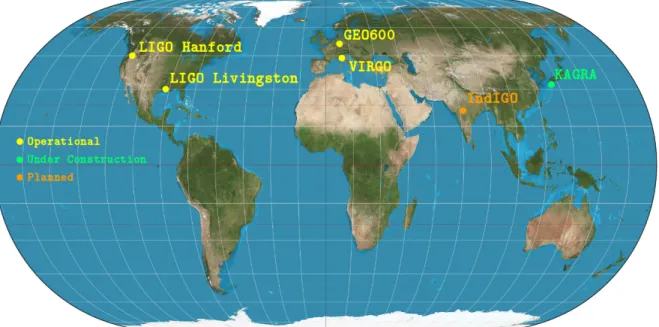
To date, we count a global network of four operational IFOs, namely the German-British detector GEO 600 (with an arm length of 600m [22]), the two LIGO ob-servatories in the United States (with 4km arms [23]) and the Virgo project of the European Gravitational Observatory (with 3km arms [24]). Future observatories are already under construction (KAGRA in Japan [25]) or planned (IndIGO in India [26]). It is worth mentioning LISA, an ESA mission with NASA participation, which objective is to deploy a several million kilometers IFO in space [27]. Figure 1.6 shows a world-map of the different sites for the different projects mentioned. In chapter 2, we will present in more depth the LIGO project specifically.
1.4. DETECTORS AROUND THE WORLD
Figure 1.5: Overview of a Fabry-Perot Michelson IFO, coupled with a power recycling cavity at the input, and a signal recycling cavity at the output.
Chapter 2
LIGO
2.1
Introduction
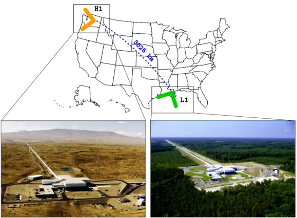
LIGO, which stands for Laser Interferemeter Gravitational-Wave Observatory, is an American project funded by the US National Science Fundation and overseen jointly by the California Institute of Technology (Caltech) and the Massachusetts Institute of Technology (MIT). Started in 1992, this project is the world’s largest observatory, with two identical 4km-arms long detectors, one in Hanford (Washington State) and one in Livingston (Louisiana State). Pictures of the detectors are shown in figure 2.1. The project went through two distinct periods. The first version of LIGO’s IFOs, referred as Initial LIGO [28, 29], took place from the late 1990s to 2008. It was intended as a ’pathfinder’, used to test and spur the technologies required. The initial LIGO detectors reached their design sensitivity in 2006 [30] and have produced astrophysical interesting results [31, 32, 33], but no detection. In 2008 started the second and current period, referred as Advanced LIGO [34]. Advanced LIGO uses the initial LIGO buildings and vacuum systems but otherwise consist of completely new instruments, which give better sensitivity [35]. Currently, Advanced LIGO has the world most sensitive instruments with a strain sensitivity of ∼ 10−23/√Hz at 100Hz [36]. Thanks to this sensitivity, Advanced LIGO claims six detections to this date.
Figure 2.1: Location and orientation of the LIGO detectors at Hanford, WA (H1) and Livingston, LA (L1).
2.2
Detections
2.2.1
GW150914
Advanced LIGO achieved a milestone on September 14, 2015 at 09:50:45 UTC by observing a GW signal for the first time [37]. One hundred years after Einstein’s theory of general relativity, the two detectors of LIGO simultaneously measured a transient GW signal of two black holes collapsing with each other, as shown in figure 2.2 (phenomenon usually referred as a binary black hole merger, or BBH merger). The detectors were sensitive enough to observe a signal for 0.2 seconds, from 35 to 250Hz with a peak strain of 1 × 10⁻²¹. Based on relativity models, this signal tells us that a BBH system, distant by 410Mpc (i.e. 1.3 billion light-years) from Earth, and composed by two black holes with masses of 36M and 29M (i.e. 36 and 29 times
the mass of our Sun), merged to form a single 62M mass black hole. During that
process, the equivalent of 3M was released as radiated GW. It is to this date the
2.2. DETECTIONS
Figure 2.2: From reference [37]. Left panel: Estimated strain amplitude produced by the GW150914 event, as the black holes collapsed with each other (numerical relativity model). Righ panel: mea-sured signal by the L1 and H1.
2.2.2
GW151226
On December 26, 2015, both LIGO detectors observed the signal produced by the coalescence of a BBH system [38]. The system, distant by 440Mpc (i.e. 1.4 billion light-years), was composed by 14.2M and 7.5M masses black holes, and form a
final single black hole of 20.8M (equivalent of 0.9M radiated as GW). The detected
signal lasted for 1 second in the IFOs from 35 to 450Hz, and reach a peak gravitational strain of 3.4 × 10⁻²². The signal measured by the LIGO IFOs is shown in figure 2.3.
Figure 2.3: From reference [38]. Measured signal filtered between [30-600Hz] for H1 (left plot) and L1 (right plot) with the best-match template from numerical models (in black).
2.2.3
GW170104
On January 4, 2017, a 31.2M and a 19.4M black hole merged to form a 48.7M
black hole [39]. During that process, almost 2M of GW was radiated. The LIGO
detectors observed a 0.3s signal from 160 to 199Hz with a peak strain amplitude of ∼ 5 × 10⁻²², as shown in figure 2.4.
Figure 2.4: From reference [39]. Measured signal filtered between [30-600Hz] for H1 (left plot) and L1 (right plot) with the best-match template from numerical models (in black).
2.2.4
GW170608
On June 8, 2017, both LIGO detectors observed the merging of a BBH system, made of a 12M and a 7M black hole [40]. The merging formed a 18M black hole,
releasing the equivalent of 1M of GW in the process. The detectors caught a 2s
signal from 30 to 500Hz with a peak strain amplitude of ∼ 4 × 10⁻²²
Figure 2.5: From reference [40]. Power maps of LIGO strain data at the time of GW170608. The characteristic upward-chirping morphology of a BBH driven by GW emission is visible in both detectors, with a higher signal amplitude in LHO.
2.2. DETECTIONS
2.2.5
GW170814
On August 14, 2017, a new milestone was reached with the first joint detection between LIGO and VIRGO [41]. The signal was emitted in the final moments of the coalescence of two black holes of 31M and 25M , about 540Mpc away (1.8 billion
light-years).
This detection marks the beginning of the international GW network, but also shows the advantages of having three detectors. Thanks to VIRGO, the sky localization of the event went from 1160deg2 with only two detectors to 60deg2, as shown in figure 2.6.
Figure 2.6: Having three detectors allowed a huge improvement in the localization of the signal’s origin. The origin is constraint to the area showed in yellow, just above the Magellanic clouds and generally toward the constellation Eridanus. Credits: apod.nasa.gov
.
2.2.6
GW170817
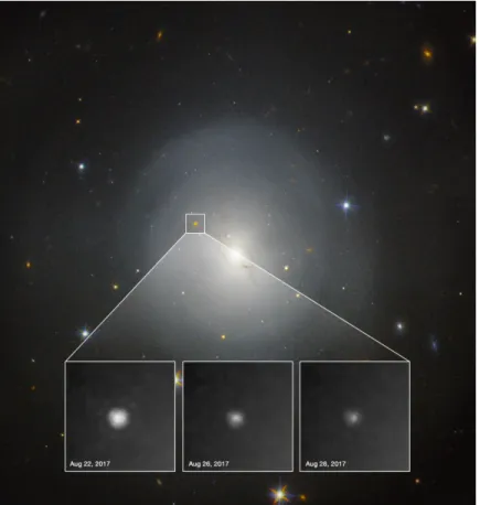
On August 17, 2017, not only LIGO observed the merger of two neutron stars (bi-nary neutron stars merger, or BNS merger) for the first time, but also this event was seen by many (∼ 70) electromagnetic telescopes [42]. Unlike all previous GW detections, which had no detectable electromagnetic signal, this event has an electro-magnetic counterpart. 1.7 seconds after LIGO’s detection, a short gamma-ray burst was observed by FERMI and Interval telescopes [43, 44]. 11 hours later, many tele-scopes, from radio to X-ray wavelengths, observed an optical transient matching the characteristics and location of the GW, as shown in figure 2.7.
It was the longest (more than a minute) and loudest (peak strain at 7.5 × 10⁻²⁰) signal observed by LIGO, marking the beginning of multi-messenger astronomy. All
the detections are summarized in table 2.1
Figure 2.7: Hubble picture of the galaxy NGC 4993 with inset showing the gamma ray burst associated with GW170817 over 6 days. Credits: NASA and ESA).
Table 2.1: Summary of LIGO detections to date.
Event Seen Source Masses GW Peak Distance
by energy strain m1= 36M GW150914 H1,L1 BBH m2= 29M 3M 1 × 10⁻²¹ 410Mpc mfinal= 62M m1= 14.2M GW151226 H1,L1 BBH m2= 7.5M 0.9M 3.4 × 10⁻²² 440Mpc mfinal= 20.8M m1= 31.2M GW170104 H1,L1 BBH m2= 19.4M 2M 5 × 10⁻²² 880Mpc mfinal= 48.7M m1= 12M GW170608 H1,L1 BBH m2= 7M 1M 4 × 10⁻²² 340Mpc mfinal= 18M m1= 31M GW170814 H1,L1,V1 BBH m2= 25M 3M 5 × 10⁻²² 540Mpc mfinal= 53M m1= 2.26M GW170818 H1,L1,V1 BNS m2= 1.36M 0.33M 7.5 × 10⁻²⁰ 40Mpc EM partners mfinal= 3.29M
2.3. THE LIGO INTERFEROMETER
2.3
The LIGO interferometer
The Advanced LIGO detectors are designed to detect GWs from distant astrophysical sources in the frequency range from 10Hz to 5kHz. Despite some minor technical dif-ferences, the detectors are identical. They are based on the dual recycled Fabry-Perot Michelson design described in section 1.3.3. The laser source is a Nd:YAG master-oscillator-power-amplifier emitting up to 180W at a single wavelength of 1064nm [45]. The laser power and frequency are actively stabilized with a transmissive ring cavity, called pre-mode cleaner (PMC). This cavity stabilizes the power fluctuations of the beam to ∼ 10−7/√Hz at 100Hz [46]. This stabilized beam passes through an input mode cleaner (IMC) and a faraday isolator (FI) before reaching the PRM. The IMC is a 33m (round-trip) triangular Fabry-Perot cavity which cleans the spatial profile and the polarization of the laser beam [47]. At the output side, an output mode cleaner (OMC) is present after the SRM to reject unwanted spatial and frequency components of the light, before the signal is detected by the main photodetector. Fi-nally, to avoid acoustical coupling and reduce phase fluctuations from light scattering off residual gas [48], the main optical components and beam paths are enclosed in an ultra-high vacuum system (10−6− 10−7Pa).
An accurate scheme of the LIGO IFO is shown in figure 2.8, with its optical param-eters summarized in table 2.2. At full power, the IFO is designed to operate with an input laser power of 125W, which corresponds to ∼ 1MW of circulating power in each arm.
Table 2.2: List of the Advanced LIGO optical parameters
Parameter (unit) Value
Laser wavelength (nm) 1064
Input power at PRM (W) up to 125
Arm cavity length (m) 3994.5
Arm cavity finesse 450
Power recycling cavity length (m) 57.6
Signal recycling cavity length (m) 56.0
IMC length - round trip (m) 32.9
OMC length - round trip (m) 1.13
IMC finesse 500
OMC finesse 390
2.4
Noise
To reach the LIGO designed sensitivity, there are stringent requirements on the noise. In this section, we present the major limiting noise sources for the different frequency bands, from 5Hz to 5kHz. Since the IFOs are designed to detect the strain amplitudes of GWs, it is convenient to talk about the equivalent strain amplitude for each given noise.
2.4.1
Seismic noise
At low frequency (i.e. < 10Hz), the predominant noise is due to seismic motion: the residual seismic vibrations impose displacement noise on the test masses of the detectors. At 1Hz and above, anthropogenic activities generate non-negligible surface vibrations. We typically measured a ground motion of ∼ 10−9m/√Hz at 10Hz. The [0.1-1Hz] bandwidth is dominated by the Earth natural seismic background, referred to as microseism. It is caused by meteorological storms in the oceans and complex atmospheric disturbances [49]. Microseism is a constant disturbance composed by a primary and secondary (or double-frequency) microseism, covering two distinct frequencies: ∼ 75mHz and ∼ 150mHz respectively. The secondary microseism is the largest seismic disturbance, which varies from season to season (winter being the worst) and from site to site (L1 being the worst). A rough estimate would be a motion of ∼ 10−6m/√Hz at 150mHz. The motion below 0.1Hz is less important compared to the other frequencies, except during earthquakes (see chapter 3). It is hard to measure the ground behavior in this band due to technological limitations (namely noise and tilt re-injection in the ground seismometers). However, we do believe that most of the motion is due to rotation induced by wind tilting the observatories’ buildings [50]. Tilt will be discussed in more details in chapter 3.
2.4. NOISE
To overcome the seismic motion, it is filtered using a combination of passive and active stages. The test masses are suspended by quadruple pendulums [51], which are mounted on multistage active platforms [52]. Overall, there are seven stages of isolation between the test masses and the ground, providing almost 1/f10 isolation in
the detection bandwidth. The seismic noise is represented in figure 2.9.
Figure 2.9: Estimation of the seismic noise in the LIGO detection bandwidth. The peak at 10Hz corresponds to the highest resonant mode of one of the isolation stages (bounce mode). Figure generated by the GWINC (Gravitational-Wave Interferometer Noise Calculator) package [53].
2.4.2
Gravity gradient noise
The local fluctuations of the gravitational field around the vacuum chambers couple with the test masses as a noise force [54]. These fluctuations, known as gradient noise or Newtonian noise, are due to passing seismic waves and surface phenomenon changing the local density of Earth. We can define the Newtonian noise transfer function T (f ) by:
T (f ) = x(f )˜ ˜
W (f ) (2.1)
with ˜x(f) = |∆x(ω)| the displacements of the test masses and ˜W(f) = |∆X(w)| the motions in Earth produce by seismic activity. From reference [55], an estimate of
T (f ) is:
T (f ) = 4πGρ
p(ω − ω0)2+ ω2/τ2
β(f ) (2.2)
where ρ is the density of the earth near the test mass, ω is the angular frequency of the seismic waves and ω0 and τ are the resonant frequency and damping time of
the test mass pendulums. The parameter β(f) is a modeled, frequency dependent, dimensionless parameter related to environmental conditions (see [55] for more details on β(f) calculation). An estimate of the Newtonian is shown on figure 2.10.
There is currently no strategy implemented to mitigate this noise, but an array of seismometers has been installed at H1 to do active noise subtraction in the near future [56].
Figure 2.10: Estimation of the Newtonian noise in the LIGO detection bandwidth. The change of slope around 10Hz is due to the different sources of noise. Below 10Hz, the noise is mostly generated by seismic waves (seismic gravity gradient noise), while above 10Hz, it is created by atmospheric disturbances (atmospheric gravity gradient noise).
2.4.3
Suspension and coating thermal noise
In a mechanical system, the loss is characterized by the conversion of mechanical energy into thermal energy. Based on the fluctuation-dissipation theorem of Callen
2.4. NOISE
and Welton [57], the reciprocal statement is true: thermal fluctuations are sponta-neously converted into mechanical fluctuations, creating displacement noise. These thermal fluctuations could be generated by externally imposed temperature variations (e.g. the laser beam on the test mass surface [58]), or could be driven by internal fluctuations (Brownian motion [59]). In both cases, we call this noise thermal noise. There are three main thermal noise sources in LIGO. The first one is the thin sus-pension fibers holding the test masses [60]. The small diameter of these fused silica fibers (d = 400µm) conceive non-negligible thermal fluctuations, especially via ther-moelastic damping [61]. Thermal noise is also generated by the optical coatings of the test masses (the front face of the mirrors are covered with multilayers of silica and titania-doped tantala [62] to provide the required high reflectivity). Finally, noise is generated by the substrates of the test masses, but with less impact for Advanced LIGO [63].
The fibers, coatings and test masses have been designed to limit the thermal noise re-injection in the LIGO IFOs. The noise is shown in figure 2.11.
Figure 2.11: Estimation of the thermal noise. The noise associated with the fibers is plotted in blue. The several high-frequency peaks correspond to the different violin modes and harmonics of the fibers. The noise associated with the mirrors is shown in red (it is grandly due to the coating).
2.4.4
Residual gas noise
Despite the ultra-high vacuum system of Advanced LIGO, the statistical fluctuations in the density of the residual gas create non-negligible noise. Residual gas can dis-turb the laser field’s phase as a gas molecule moves through the beam. The model developed by Zucker et al. [48] predicts the power spectral density of the arm length variation to be: SLarm(f ) = 4ρ(2πα)2 ν0 Z Larm exp[−2πf w(z)/ν 0] w(z) dz (2.3)
for a particular molecule with number density ρ, speed ν0 and polarizability α. w(z)
is the beam’s Gaussian radius. The residual gas noise is plotted in figure 2.12.
Figure 2.12: Estimation of the excess gas noise.
2.4.5
Quantum noise
In 1927, Heisenberg introduced a fundamental limit to the precision with which one can determine the position of a free mass. This is known as Heisenberg’s uncertainty principle, and it’s defined by:
![Figure 2.2: From reference [37]. Left panel: Estimated strain amplitude produced by the GW150914 event, as the black holes collapsed with each other (numerical relativity model)](https://thumb-eu.123doks.com/thumbv2/123doknet/14676163.742442/46.918.155.746.109.356/figure-reference-estimated-amplitude-produced-collapsed-numerical-relativity.webp)