HAL Id: tel-01565969
https://tel.archives-ouvertes.fr/tel-01565969
Submitted on 20 Jul 2017
HAL is a multi-disciplinary open access
archive for the deposit and dissemination of sci-entific research documents, whether they are
pub-L’archive ouverte pluridisciplinaire HAL, est destinée au dépôt et à la diffusion de documents scientifiques de niveau recherche, publiés ou non,
the CERN Super Proton Synchrotron
Alexandre Samir Lasheen
To cite this version:
Alexandre Samir Lasheen. Beam Measurements of the Longitudinal Impedance of the CERN Super Proton Synchrotron. Accelerator Physics [physics.acc-ph]. Université Paris Saclay (COmUE), 2017. English. �NNT : 2017SACLS005�. �tel-01565969�
NNT : 2017SACLS005
THÈSE DE DOCTORAT DE L’UNIVERSITÉ PARIS-SACLAY
PREPARÉE À L’UNIVERSITÉ PARIS-SUD
ÉCOLE DOCTORALE N°576
Particules Hadrons Énergie et Noyau : Instrumentation, Image, Cosmos et Simulation (PHENIICS)
Spécialité de doctorat : Physique des accélérateurs
Par
M. Alexandre Samir Lasheen
M
ESURES DE L
’I
MPÉDANCE
L
ONGITUDINALE
AVEC LE
F
AISCEAU DU
CERN S
UPER
P
ROTON
S
YNCHROTRON
Thèse présentée et soutenue à Orsay, le 13 Janvier 2017
Composition du jury:
Dr. Guy Wormser, LAL, Président du jury
Prof. Costel Petrache, CSNSM, Directeur de thèse Dr. Elena Shaposhnikova, CERN, Co-directrice de thèse Prof. Jean-Marie De Conto, LPSC, Rapporteur
Prof. Mauro Migliorati, Univ. La Sapienza, Rapporteur Dr. Elias Métral, CERN, Examinateur
Dr. Ryutaro Nagaoka, SOLEIL, Examinateur Dr. Olivier Napoly, CEA, Examinateur
À ma famille, à Marie. . .
Acknowledgements
First and foremost, I would like to thank Elena Shaposhnikova for giving me the chance to do my PhD under her supervision. During these three years and since the very first day, her advice and guidance was always relevant and in my interest to progress. Thanks for sharing with me your immense knowledge, for your kindness and your endless curiosity that I will keep as a great source of inspiration as a researcher and for my life in general.
I would like also to thank Costel Petrache, for accepting to be my supervisor on behalf of the university. Costel was also my supervisor as a master’s degree student, and supported me when I applied for a PhD at CERN. Thanks for always supporting me for my last steps as a student and the first ones as a researcher, allowing me to do this exciting work.
I am thankful to the members of the jury: Prof. Jean-Marie De Conto and Prof. Mauro Migliorati for accepting the important task to review the manuscript as referees, Dr. Elias Métral, Dr. Ryutaro Nagaoka and Dr. Olivier Napoly as members of the examining committee and Dr. Guy Wormser as president of the jury. Thanks for your interesting questions and remarks on my work.
The work presented here would not have been possible without the help of many colleagues. Since my arrival, I could always count on my exceptional office mates, Theodoros Argyropoulos and Juan Esteban Müller. Theo and Juan showed me all the tricks I needed to know to be efficient in my work, as well as being remarkable people. Thanks to both of you for making every working day enlightening, enjoyable and for your friendliness. In that respect, I would also like to thank Helga Timko for introducing me to the topic at my arrival, and Joël Repond to whom I introduced the topic in the end of my PhD.
Special thanks to Thomas Bohl and Steve Hancock, for helping me to tame the RF systems of the whole injector chain and showing me all I needed to know to perform autonomously beam measurements. Thanks for the countless hours you devoted me in the SPS BA3 Faraday cage and in the CPS island in the CCC, to share your knowledge with me.
My work was done in the Beams and RF section at CERN. I would like to thank all the members of this section where I felt well integrated and part of a great project, with special thanks to Simon Albright and James Mitchell for proofreading my thesis. I would like also to thank the students passing by and always bringing a great atmosphere.
The simulation code BLonD was used for all the simulations done during my PhD. The development of this code was the result of a fruitful collaboration, and I would like to thank Danilo Quartullo and Konstantinos Iliakis for maintaining and optimising the code, as well as Helga, Juan, Joël and Simon for their development.
The work presented in this thesis relies on the important work of the impedance team at CERN. Extensive efforts were devoted to develop the SPS impedance model, mainly by Jose Varela, Benoit Salvant, Carlo Zannini, with additional contributions from Thomas Kaltenbacher, Patrick Kramer, Christine Vollinger, Toon Roggen and Rama Calaga. Many thanks to all of you and for the fruitful discussions.
All the measurements presented in this thesis were made possible thanks to the help of Giovanni Rumolo and Hannes Bartosik as MD coordinators. Thanks for your confidence in my work, and for the beam time you gave me. I am also thankful to the SPS and CPS operation teams, for giving me their time to adjust the machine parameters.
Pour finir je tiens à remercier ceux par qui tout a commencé. Merci à mes parents et ma sœur pour leur soutien inconditionnel depuis mes tout premiers pas. Merci à toi Marie de m’avoir accompagné au quotidien et d’avoir donné tout son sens à ma vie.
Merci finalement à tous ceux qui ne sont pas nommés ici mais qui ont contribué à leur façon, par leurs encouragements, leur amitié, et leur bienveillance...
Abstract
One of the main challenges of future physics projects based on particle accelerators is the need for high intensity beams. However, collective effects are a major limitation which can deteriorate the beam quality or limit the maximum intensity due to losses. The CERN SPS, which is the last injector for the LHC, is currently unable to deliver the beams required for future projects due to longitudinal instabilities.
The numerous devices in the machine (accelerating RF cavities, injection and extraction magnets, vacuum flanges, etc.) lead to variations in the geometry and material of the chamber through which the beam is travelling. The electromagnetic interaction within the beam (space charge) and of the beam with its environment are described by a coupling impedance which affects the motion of the particles and leads to instabilities for high beam intensities. Consequently, the critical impedance sources should be identified and solutions assessed. To have a reliable impedance model of an accelerator, the contributions of all the devices in the ring should be evaluated from electromagnetic simulations and measurements.
In this thesis, the beam itself is used to probe the machine impedance by measuring the synchrotron frequency shift with intensity and bunch length, as well as the line density modulation of long bunches injected with the RF voltage switched off. These measurements are compared with macroparticle simulations using the existing SPS impedance model, and the deviations are studied to identify missing impedance sources and to refine the model. The next important step is to reproduce in simulations the measured single bunch instabilities during acceleration, in single and double RF system operation. Thanks to the improved impedance model, a better understanding of instability mechanisms is achieved for both proton and ion beams.
Finally, as the simulation model was shown to be trustworthy, it is used to estimate the beam characteristics after the foreseen SPS upgrades the High Luminosity-LHC project at CERN. Key words: particle accelerators, longitudinal beam dynamics, beam-based measurements, CERN SPS, beam coupling impedance, beam instabilities
Résumé
Un des défis pour les futurs projets en physique basé sur les accélérateurs de particules est le besoin de faisceaux à hautes intensités. Les effets collectifs sont cependant une limitation majeure qui peuvent détériorer la qualité du faisceau ou limiter l’intensité maximale à cause des pertes. Le CERN SPS, qui est le dernier injecteur pour le LHC, n’est actuellement pas en mesure de délivrer les faisceaux requis pour les futurs projets à cause des instabilités longitudinales.
Les nombreux équipements dans la machine (les cavités RF accélératrices, les aimants d’in-jection et d’extraction, les brides de vide, etc.) entrainent des variations dans la géométrie et les matériaux de la chambre dans laquelle le faisceau transite. Les interactions électroma-gnétiques internes au faisceau (charge d’espace) et du faisceau avec son environnement sont représentées par une impédance de couplage qui affectent le mouvement des particules et mènent à des instabilités pour des intensités élevées de faisceau. Par conséquent, les sources d’impédance critiques doivent être identifiées et des solutions évaluées. Pour avoir un modèle d’impédance fiable d’un accélérateur, les contributions de tous les équipements dans l’anneau doivent être évaluées à partir de simulations et de mesures électromagnétiques.
Dans cette thèse, le faisceau lui-même est utilisé comme une sonde de l’impédance de la machine en mesurant le déplacement de la fréquence synchrotronique avec l’intensité et la longueur du paquet, ainsi que la modulation de longs paquets injectés avec la tension RF éteinte. Ces mesures sont comparées avec des simulations par macroparticules en utilisant le modèle d’impédance du SPS existant, et les déviations sont étudiées pour identifier les sources d’impédance manquantes pour raffiner le modèle.
L’étape suivante consiste à reproduire en simulations les instabilités mesurées pour un paquet unique durant l’accélération. Grâce à l’amélioration du modèle d’impédance, une meilleure compréhension des mécanismes de l’instabilité est rendue possible pour les faisceaux de protons et d’ions.
Finalement, le modèle pour les simulations étant digne de confiance, il est utilisé pour estimer les caractéristiques du faisceau après les améliorations prévues du SPS pour le projet High Luminosity-LHC au CERN.
Mots clefs : accélérateurs de particules, dynamique longitudinale du faisceau, mesures avec le faisceau, CERN SPS, impédance de couplage, instabilités du faisceau
Contents
Acknowledgements i
Abstract - Résumé iii
Introduction 1
The CERN accelerator complex . . . 1
The CERN Super Proton Synchrotron and beam instabilities . . . 3
The SPS beam coupling impedance . . . 6
Beam measurements of the impedance . . . 9
Thesis outline . . . 9
1 Synchrotron motion with intensity effects 11 1.1 Introduction . . . 11
1.2 Longitudinal equations of motion . . . 11
1.2.1 Synchronism condition in synchrotrons . . . 11
1.2.2 Energy gain in the RF cavity . . . 13
1.2.3 Slippage in arrival time to the RF cavity . . . 15
1.2.4 Induced voltage . . . 16
1.2.5 Single particle motion . . . 19
1.2.6 Hamiltonian of the synchrotron motion . . . 20
1.2.7 Coherent bunch motion and instabilities . . . 23
1.3 Beam measurements of the impedance . . . 23
1.3.1 Synchronous phase shift and energy loss . . . 24
1.3.2 Synchrotron frequency shift . . . 25
1.3.3 Bunch lengthening . . . 26
1.3.4 Instability threshold and growth rate . . . 27
1.4 Conclusions . . . 28
2 Quadrupole frequency shift as a probe of the reactive impedance 29 2.1 Introduction . . . 29
2.2 Quadrupole synchrotron frequency shift . . . 30
2.2.1 Synchrotron frequency for particles with large oscillation amplitude . . 31
2.2.2 Incoherent synchrotron frequency shift . . . 32
2.3 Measurements of the quadrupole frequency shift . . . 41
2.3.1 Setup . . . 41
2.3.2 Data analysis and results . . . 42
2.4 Particle simulations . . . 45
2.4.1 BLonD simulations . . . 45
2.4.2 Evaluation of the missing impedance . . . 46
2.5 Conclusions . . . 48
3 Longitudinal Space Charge in the SPS 49 3.1 Introduction . . . 49
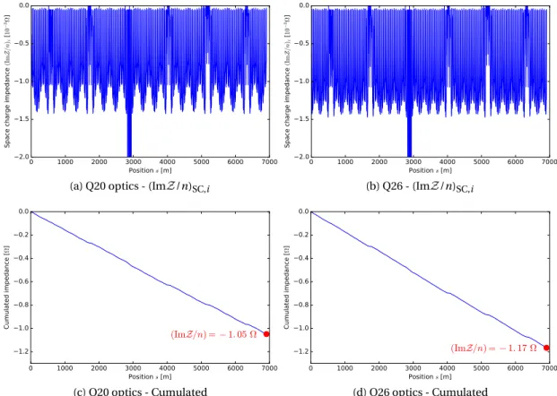
3.2 Evaluation of the space charge at all positions in the ring . . . 51
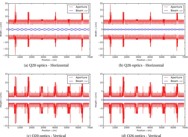
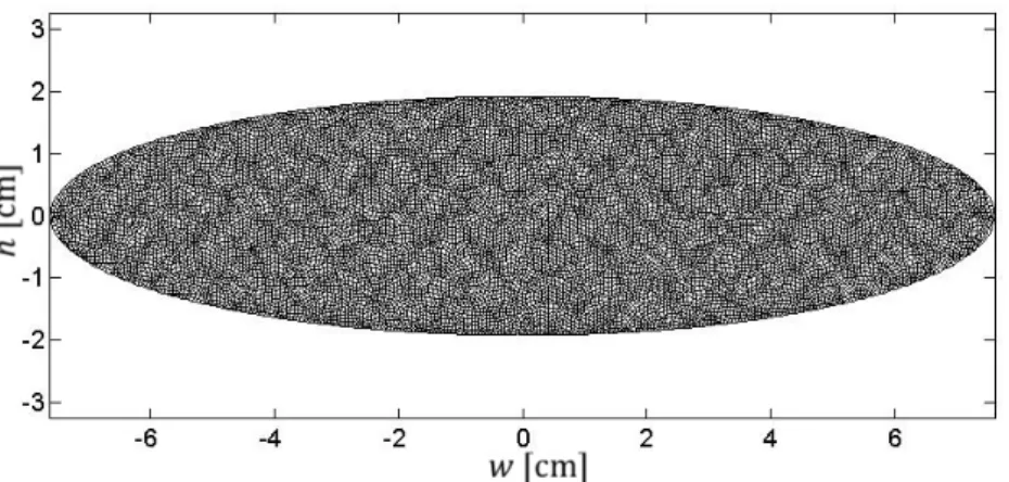
3.2.1 Aperture geometry along the ring and bunch distribution . . . 51
3.2.2 Evaluation of the space charge using averaged beam and aperture param-eters . . . 53
3.2.3 Evaluation of the space charge along the ring using a simplified geometry 53 3.2.4 Evaluation of the space charge along the ring with the LSC code . . . 54
3.2.5 Summary of the methods to compute the geometrical factor . . . 55
3.3 Longitudinal space charge during the cycle . . . 55
3.3.1 Dependence on energy and bunch length . . . 56
3.3.2 Dependence on the geometrical factor . . . 58
3.4 Conclusions . . . 59
4 Measurement of High Frequency Impedance Sources 61 4.1 Introduction . . . 61
4.2 Microwave instability with RF off . . . 62
4.3 Measurements . . . 65
4.3.1 Setup . . . 65
4.3.2 Data analysis . . . 66
4.4 Particle simulations . . . 72
4.4.1 BLonD simulations . . . 72
4.4.2 Effect of the initial bunch distribution . . . 74
4.5 Conclusions . . . 76
5 Single bunch instabilities during the SPS ramp 79 5.1 Introduction . . . 79
5.2 Proton bunches . . . 79
5.2.1 Beam instabilities in single RF operation . . . 80
5.2.2 Bunch lengthening from potential-well distortion . . . 84
5.2.3 Beam instabilities in double RF operation . . . 86
Contents
6 Applications for future projects 97
6.1 Introduction . . . 97
6.2 Simulation setup . . . 97
6.3 Present configuration . . . 98
6.4 Projection for future RF configurations . . . 100
6.5 Conclusions . . . 101
Summary and conclusions 103
A Synthèse en français 105
Introduction
The CERN accelerator complex
Particle accelerators were originally designed to provide beams for nuclear and particle re-search, fulfilling various needs in terms of beam intensity, energy, as well as particle types. Many more uses of particle accelerators were then found, ranging from industrial applications to particle therapy for cancer treatment. Over the past years, technological progression have allowed an increased performance of particle accelerators, leading to important discoveries. The continuous need for higher beam intensities leads to reach the limits of machine perfor-mances defined by the electromagnetic fields induced by the beam. One of these limits are beam instabilities, which can degrade the beam quality and eventually lead to particle losses, and hence represent a limitation for future projects.
The European Organisation for Nuclear Research (CERN) hosts a wide chain of particle ac-celerators, including the well-known Large Hadron Collider (LHC) and many lower energy rings. The complete schematic map of the complex is shown in Fig. I.1. One of the most recent highlights at CERN is the discovery of a new boson compatible with the Higgs boson, produced from the collision of the two proton beams of the LHC at an energy of 3.5 TeV (7 TeV in the centre of mass) and measured by the ATLAS and CMS detectors [1, 2].
The number of events registered in the LHC experiments is given by the luminosityL, which is determined by the number of particles in the colliding bunches Nb, withL∝ Nb2. To increase
the number of events and therefore the probability to detect particles of interest, high bunch intensities are needed. This is also one of the requirements of the High Luminosity-LHC (HL-LHC) project [3], where the goal is to increase the luminosity by a factor of 10. One of the ingredients to achieve this aim is an increase in bunch intensity by a factor of 2 with respect to present operation. However, the collective (or intensity) effects will also increase, and this goal is currently not achievable without machine upgrades.
The LHC is filled by an injector chain consisting of several particle accelerators. Their role is to accelerate the beam up to the energy acceptable by the LHC. Protons are first accelerated in the Linear Accelerator 2 (LINAC2, up to a kinetic energy of 50 MeV), the Proton Synchrotron Booster (PSB, up to 1.4 GeV), the Proton Synchrotron (PS, up to 25 GeV) and finally the Super Proton Synchrotron (SPS, up to 450 GeV). The second role of the injector chain is to shape the
Figure I.1 – The CERN accelerator complex (© CERN).
beam in several bunches, with the time structure required by the LHC experiments. A single bunch is formed in the PSB and sent to the PS, where this bunch is split into several bunches using RF manipulations. In the nominal operation, 6 PSB bunches are split into 72 bunches spaced by 25 ns, where each bunch is composed of 1.2 × 10¹¹protons. Up to four batches of 72 bunches are injected from the PS into the SPS, and many injections are done to fill the LHC with the nominal number of bunches per beam. When the two counter-rotating beams are ready in the LHC, they are finally accelerated from 450 GeV to collision energy, which was 3.5 TeV during the LHC run 1 (2010-2013) and since the restart in 2015 is 6.5 TeV .
Each ring of the LHC injector chain has different limitations due to intensity effects. If a single accelerator in the chain is limited in its performance, the required beam is not able to reach the LHC and fulfil the needs of the experiments. The goal of the LHC Injectors Upgrade (LIU) project [4] is to identify the limitations and to find and implement solutions which would allow delivery of the beam required for the HL-LHC project. Presently, one of the main bottlenecks is the SPS due to beam loading and longitudinal instabilities (more details are below). The injector chain is also able to accelerate ions for collisions in the LHC and fixed target experiments. The LIU project includes an upgrade of the injector chain for ion beams [5] for the HL-LHC project (Pb-Pb and p-Pb collisions). The ion beam follows a different path
The CERN Super Proton Synchrotron and beam instabilities
up to a kinetic energy of 4.2 MeV/u), the Low Energy Ion Ring (LEIR, up to 72 MeV/u), then follows the same path as the proton beam in the PS (up to 5.9 GeV/u) and finally the SPS (up to 176.4 GeV/u).
Many other physics experiments are located at different stages in the CERN accelerator chain and also rely on the low energy accelerators. A relevant example in the frame of this thesis is the Advanced WAKefield Experiment (AWAKE) [6] at extraction from the SPS. The AWAKE project aims at studying plasma wakefield acceleration, which is expected to give much higher accelerating gradients with respect to conventional methods (order of GV/m in plasma wakefield acceleration, in comparison with order of MV/m in RF acceleration). In the future, this could lead to more compact particle accelerators for physics studies at the high energy frontier. The requirement to the SPS from the AWAKE project is a single bunch with a high density (small bunch length and high bunch intensity) at 400 GeV to be sent into a plasma chamber. However, the achievable bunch parameters are also limited by beam instabilities. Both the HL-LHC and AWAKE projects rely on a successful acceleration of the required beam in the SPS. The intensity effects need to be well controlled since the delivered beam should be reproducible from one cycle to another and remain within the specifications. Therefore, it is necessary to study the intensity effects in the SPS, and in particular beam instabilities in the longitudinal plane. To do so, an accurate impedance model of the SPS is essential to identify the sources of the instabilities, and to hence find possible cures.
The CERN Super Proton Synchrotron and beam instabilities
The SPS was commissioned in 1976 and is presently the second largest accelerator at CERN, with a circumference of 6.9 km. During those 40 years, it was used as a proton-antiproton collider (Sp ¯pS), as an injector for the Large Electron Positron collider (LEP), and provided beams for various fixed target experiments (e.g., North Area experiments, CNGS, HiRadMat). The SPS accelerated all kind of particles: protons, antiprotons, electrons, various ions. It is also used as a test bench for new accelerator physics concepts and devices, an example being the crab-cavities which will be used in the HL-LHC project to increase the luminosity [3]. These cavities will be tested in the SPS before installation in the LHC. Major scientific discoveries were done using the SPS beam, for example the W and Z bosons in 1983 [7, 8]. The present SPS machine parameters are shown in Table I.1.
The versatility of the SPS was made possible thanks to many upgrades of the machine. However, this longevity implies that some elements in the machine were not designed in prevision of the requirements of the HL-LHC project, and are now a problem. The many devices, present in a particle accelerator, introduce some changes in the geometry of the vacuum chamber through which the beam is travelling. A particle passing through a cavity-like structure will deposit some energy in the form of an electromagnetic perturbation (wakefield). The frequency distribution of the wakefield, called the beam coupling impedance (or simply impedance below) depends on the geometry of the surroundings. This perturbation can affect the motion
of the following particles within the same bunch (single bunch effects), the following bunches bunch effects), and even the same bunches at the following revolution turn (multi-turn effects). Due to the long history of the SPS, many impedance sources are present in the machine and are responsible for the present machine performance limitations. The intensity effects are different in transverse and longitudinal beam dynamics. In the SPS the limitations of the LHC beam are mainly due to the effects in the longitudinal beam dynamics, which are the main focus of this thesis. The beam parameters presently achieved in the SPS together with the goals of the LIU project are shown in Table I.2.
Table I.1 – Machine parameters of the CERN SPS for the LHC (protons and ions) and AWAKE beams. Values separated with / correspond to injection/extraction. Values with ∼ are approxi-mate and have small variations during the ramp.
Parameter LHC beam LHC-ION beam AWAKE beam
Circumference C [m] 6911.50
Particle type and charge Z [e] p+ (Z=1) 208Pb82+(Z=82) p+ (Z=1)
Momentum p [Z GeV/c] 26/450 17/450 26/400
Lorentz factorγ 27.7/479.6 7.3/190.6 27.7/426.3
Transition Lorentz factorγt Q20 optics: 17.95 − Q26 optics: 22.77
Revolution period Trev [µs] ∼23.1
Main RF system
Harmonic number h200 4620
RF frequency fRF,200 [MHz] ∼ 200.2
Max. RF voltage V200 [MV] ∼ 7.5
Fourth harmonic RF system
Harmonic number h800 18480 − 18480
RF frequency fRF,800 [MHz] ∼ 800.8 − ∼ 800.8
Max. RF voltage V800 [kV] ∼ 850 − ∼ 850
Table I.2 – Beam parameters achieved in the SPS for the LHC-type beam and goals of the LIU project [4]. Values separated with / correspond to injection/extraction.
Parameter Achieved LIU target
Number of batch×bunches 4×72
Bunch spacing [ns] 25
Batch spacing [ns] 225
Bunch intensity Nb ×1011 1.3/1.2 2.6/2.4
Longitudinal emittanceεL [eVs] 0.35/0.6 <0.65
Extracted bunch lengthτL= 4σrms [ns] 1.65 <1.7
Transverse emittanceεx,y [µm] 2.36 1.89
Beam loading is one of the important SPS limitations. Beam acceleration in the SPS relies on the electric field (RF voltage) provided by a Travelling Wave RF System. It is composed
The CERN Super Proton Synchrotron and beam instabilities
is composed of several sections, so the total system includes two TWC with four sections and two TWC with five sections. The available RF voltage for the acceleration is reduced by the wakefield left by the beam in the TWC (beam loading), and for the beam intensities required for the HL-LHC project the available voltage is no longer sufficient. An upgrade of the RF system is foreseen to overcome this limitation [10]. It consists of an increase in the total number of (shorter) cavities, which together with an upgrade of the RF power supply will allow a larger RF voltage to be reached in the TWC. The increased number of sections (from 18 to 20) will be reorganised to get a total of six TWC (four TWC with three sections and two TWC with four sections). With shorter cavities, the total impedance of the RF system is lower and the beam loading effect will be reduced. After this upgrade (2021), the available RF voltage is expected to be sufficient to accelerate a beam with the intensity required for the HL-LHC project. However, other limitations exist due to other SPS impedance sources.
0
5
10
15
20
Time
t[s]
0
1
2
3
4
5
Bu
nc
h
len
gt
h
τL[n
s]
Bunch length
Min/Max
0
100
200
300
400
500
Energy [GeV]
Figure I.2 – Longitudinal instability during the SPS accelerating cycle for a batch of 72 bunches spaced by 25 ns, with an average bunch intensity of Nb≈ 1.2 × 10¹¹ppb in the Q20 optics (see
Table I.1). The average bunch length (blue) is shown, together with the beam energy (black) as a function of time. The minimum and maximum bunch lengths in the batch (red) are used as a criterion to determine when the beam becomes unstable, shown here with the vertical magenta line.
The cumulative effect of the wakefields on the beam can eventually lead to instabilities for high beam intensities. An example of measurements for the LHC type beam in the SPS is shown in Fig. I.2, where the beam becomes unstable during the acceleration ramp. The instability manifests in coherent oscillations of the bunch distribution (bunch length oscillations in this example), resulting in an uncontrolled increase of the longitudinal emittance and intensity losses. The bunch length at SPS flat top energy should not exceed 1.7 ns to minimise particle losses at injection into the LHC which has a 400 MHz RF system (twice shorter acceptable bunches compared to the SPS). In the example in Fig. I.2, the maximum bunch length within the batch is too large and this beam cannot be injected in the LHC.
The mechanism of the instability depends on multiple parameters: the longitudinal emittance, the bunch length and intensity, the RF voltage program, the optics, the impedance sources etc. The wakefields perturb the bunch motion. In the stable regime, this perturbation is damped naturally thanks to the spread in the frequencies of the individual particles com-posing the bunch (incoherent synchrotron frequency spread). This effect is called Landau damping, which was first introduced in plasma physics to describe the damping of plasma oscillations [11]. For high beam intensities, the incoherent spread is modified by the wake-fields (see Chapter 2) and this effect leads to a loss of Landau damping. In this situation, the excitation from the wakefield is not damped anymore and coherent oscillations can grow exponentially, leading to a degradation of the beam parameters. Another example is the microwave instability, which is driven by wakefields with a wavelength much shorter than the bunch length. The microwave instability manifests as a fast emittance growth [12]. To mitigate the longitudinal instabilities in the SPS, another RF system composed of two TWC tuned at a frequency of 800 MHz is available. Its only use is to stabilise the beam through Landau damping by adding non-linearities to the RF bucket [13, 14]. However, the optimisation of the RF parameters of the 800 MHz RF system is not straightforward due to the complexity of the SPS impedance. In addition, the 800 MHz RF system has a limited effect on the microwave instability [15].
Even if the beam loading limitation in the SPS is solved after the RF upgrade, initial estimations of future limitations due to instabilities, based on scaling from the present situation showed that the HL-LHC requirements may still not be reachable [16, 17]. Therefore it is essential to identify the impedance sources responsible for the instabilities, in order to find a relevant cure (e.g. damping or shielding the impedance source). In addition, it is necessary to have an accurate SPS impedance model to be able to find means of optimisation of the operational cycles, and to do more precise predictions for future projects with the help of macroparticle simulations.
The SPS beam coupling impedance
One approach to develop the impedance model of a machine is to consider each element individually and evaluate the wakefields generated by a particle passing through this element (see Section 1.2.4 for wake potentials). The impedance of this device can be found using analytical calculations (e.g. [18, 19]), electromagnetic simulations (e.g. [20, 21, 22]), and from bench measurements (e.g. [23]). In practice, a combination of the three is usually required. The model described here and shown in Fig. I.3 is the present SPS impedance model [24]. It was developed over a long period of time in parallel with beam dynamics studies, with inputs from different groups at CERN (e.g. [25, 26], with regular updates presented in the LIU-SPS Beam Dynamics Working Group [27]). The typical bunch length range in the SPS is (1.5-3) ns, therefore the frequency range of the stable bunch spectrum is within 1 GHz. The frequency range of interest for the impedance in calculations was taken up to (3-5) GHz, to account for the effect of high frequency impedance sources on the beam. There are three main groups of
The SPS beam coupling impedance
longitudinal impedance sources relevant to the studies presented in this thesis: the Travelling Wave Cavities, the injection and extraction kicker magnets and the vacuum flanges.
0.0
0.5
1.0
1.5
2.0
2.5
3.0
10
-310
-210
-110
0Re
al
pa
rt
of
im
pe
da
nc
e
R e Z[
M Ω]
0.0
0.5
1.0
1.5
2.0
2.5
3.0
Frequency [GHz]
20
15
10
5
0
5
10
15
20
Im
ag
ina
ry
p
ar
t o
f i
m
pe
da
nc
e
Im Z /n[
Ω]
Kickers
TWC200
TWC800
QF flanges
QD flanges
Space charge
Figure I.3 – The present SPS impedance model up to 3 GHz [24]: resistive part (top) and reactive part (bottom). The most relevant groups of impedance for the studies presented in this thesis are shown in different colours, while the full SPS impedance is shown in black (only for the resistive part, for clarity purpose).
The impedance of the TWC at 200 MHz and 800 MHz is responsible for the beam loading effects mentioned above. An evaluation of their impedances was done in [9, 28, 29]. In addition to the main harmonic, several High Order Modes (HOM) present in the TWC have large impedance. For the 200 MHz TWC, the most significant HOM is located at a frequency of 629 MHz, and is damped by HOM couplers. Other HOMs were also identified at higher frequencies (915 MHz and 1.13 GHz). Concerning the 800 MHz, an HOM exists at a frequency around 1.9 GHz [30].
The kicker magnets, used for the injection and extraction of the beam, are the most important contributions in terms of broadband impedance [31]. While the impedance sources can have
(a) TWC 200 MHz (b) MBA-MBA vacuum flanges
Figure I.4 – Example of impedance sources in the SPS: (a) The 200 MHz SPS Travelling Wave Cavity (inside one section, © CERN), (b) The vacuum flange between two MBA type bending magnets modelled in the CST Microwave Studio software [22].
a detrimental effect on the beam, one should also take into account that the beam can damage the devices via RF heating, which is a critical effect for the kickers. Therefore, the impedance of all extraction kickers (MKE) was reduced by serigraphy [32], which is responsible for the resonance at 44 MHz visible in Fig. I.3.
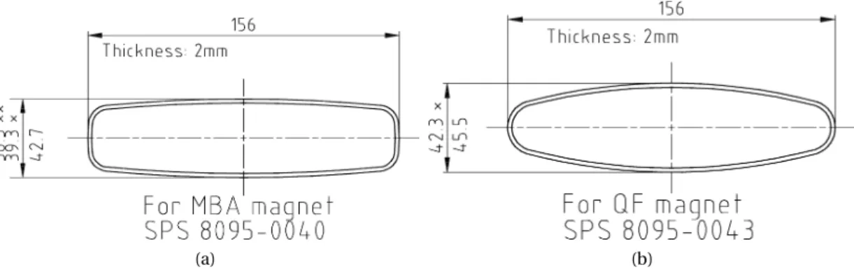
The role of the vacuum flanges is to connect the beam pipes along the ring. In the SPS, many types of vacuum chambers are used along the ring and also depend on the type of the neighbouring magnets. An example of vacuum flange between two MBA-type bending magnets is shown in Fig. I.4b. Due to the large number of these cavity-like structures in the ring, these vacuum flanges are the biggest source of resonant impedances at high frequency (above 1 GHz) in the SPS [33]. The different types of vacuum chambers can be classified in two main groups depending on their connecting beam pipe: the QF-type vacuum flanges for those close to focusing magnets (QF), and the QD-type vacuum flanges for those close to defocusing magnets (QD).
Other impedance contributions are also included in the SPS model: the resistive wall impedance (which depends on the conductivity of the beam pipe material [31]), the Beam Position Moni-tors (BPM) [34], the vacuum pumping ports [35], the Y-chambers (used to switch between two beam pipes at certain locations in the ring to put a device in and out of the ring), the tanks of the beam scrapers used to clean beam tails or halos before extraction to the LHC [27, 36]. The longitudinal space charge effect can also be modelled by an impedance, and more pre-cisely by a constant reactive impedance ImZ/n (n = f /frevwith f the frequency and frev
the revolution frequency). It is shown to be an important contribution in the study of the synchrotron frequency shift with intensity in Chapter 2. Therefore, the longitudinal space
Beam measurements of the impedance
Chapter 3) [37].
Beam measurements of the impedance
Thanks to the progress in computing tools, very detailed evaluations of the impedance sources can be done. Nevertheless, all the particularities of the impedance sources may not be taken into account (e.g. the material properties as a function of the frequency). In addition, the actual implementation of a device in the machine may be different from the ideal case in simulations or in the lab because of fabrication errors, installation constraints, or beam induced damage while operating the accelerator.
Measurements of the impedance with the beam are necessary to verify the existing impedance model. The beam characteristics are measured as a function of intensity and compared with analytical formulae or macroparticle simulations using the impedance model. Measurements using a stable beam can give information about the effective impedance corresponding to the product of the bunch spectrum with the impedance. The resistive part of the impedance ReZand the reactive part ImZhave different effects on the beam, and various methods are possible to measure them separately. The impedance can also be probed using an unstable beam. In this case, the beam spectrum also includes specific information about the main impedance source driving the instability. A review of the methods is presented in Chapter 1, where the effect of induced voltage on synchrotron motion is described.
Beam measurements can serve several purposes. The first one is to keep track of the changes in the machine after the successive installation/removal of devices (e.g. reference measurements in the SPS [38]), or to verify the correct impedance reduction of a critical impedance source (e.g. impedance reduction of the SPS pumping ports in 2000 [39]). The second purpose is to identify contributions potentially missing from the model. An example is presented in Chapter 4 where measurements allowed to reveal a source of microwave instability as a resonant impedance at 1.4 GHz, which was identified subsequently to come from the vacuum flanges [40].
The goal of this thesis was to perform beam measurements of the longitudinal impedance to benchmark the existing model. The methods used were adapted and extended to take into account the complex impedance of the SPS (see Fig. I.3). Eventually, this allowed evaluation of the possible missing impedance and its dependence on frequency.
Thesis outline
This thesis is divided into six chapters, each contains the description of one study. Altogether, the order of the chapters corresponds to the approach used in the SPS to verify and improve the longitudinal impedance model using the beam as a source of information.
The first topic is the delimitation of the contours of this thesis. It is composed of the present introduction, together with Chapter 1. It consists of a description of the problem and the motivations for this research, as well as the theoretical background necessary for the studies. Some elements in the design of the simulation code BLonD are presented together with the main equations for longitudinal beam dynamics. This code was used for all the macroparticle simulations presented in this thesis.
The main research work is presented in Chapters 2 to 5. In Chapter 2, the reactive part of the SPS impedance is evaluated from the measurements of the synchrotron frequency shift with intensity. This method was extended to scan the shift with bunch length, which allowed to identify missing impedance in the model, together with its possible dependence on frequency. This study also showed that the longitudinal space charge should not be neglected at low energy in the SPS. Consequently, the longitudinal space charge impedance was evaluated in detail and is presented in Chapter 3.
In Chapter 4, the high frequency impedance sources were probed by measuring the modu-lation of the profiles of long bunches, injected into the ring with the RF voltage switched off. This modulation, driven by microwave-like instabilities, allowed the main impedance sources responsible for microwave instabilities to be identified.
Another way to evaluate the accuracy of the impedance model is to test the ability to reproduce the measured instabilities in macroparticle simulations. Unlike the measurements presented in the previous chapters, which give a more specific information, the comparison of measured instabilities and simulations gives an evaluation of the accuracy of the impedance model as a whole. Studies done with a single proton bunch for various RF configurations (different RF programs, in single and double RF operation) are described in Section 5.2, and with a single ion bunch in Section 5.3.
The work presented in this thesis showed that simulations can reproduce reasonably all the aforementioned measurements using the present impedance model. Chapter 6 shows applications of the impedance model to explore the beam parameters achievable for the HL-LHC project, taking into account the LIU-baseline scenario of the SPS RF upgrade and impedance reduction.
1
Synchrotron motion with intensity
effects
1.1 Introduction
In this chapter the theoretical basis necessary for the thesis is reviewed, with input taken from [18, 19, 41, 42, 43]. The equations of motion were adapted to their use in the macroparti-cle tracking code BLonD (Beam Longitudinal Dynamics [44]), which was developed in collabo-ration with other members of the BE/RF group at CERN. The motivation for the development of this code was the need for an efficient and modular simulation tool to study complex problems (e.g. multi-bunch instabilities), in all the synchrotrons of the CERN accelerator complex. BLonD was designed to simulate the synchrotron motion with intensity effects, and the equations of motions were adapted to be able to simulate the various low-level RF (LLRF) systems used in operation. The code is written in Python, with optimisations in C++ for the most time demanding operations. It was benchmarked against theoretical calculations [45] and against beam measurements. It was also benchmarked against other simulation codes: ESME [46], HEADTAIL [47] and PyORBIT [48, 49].
Below, the equations of motion are presented to show the effect of the induced voltage on the synchrotron motion, for stationary and unstable bunches. First, the notion of effective impedance is introduced to show what is the effect of the resistive and reactive part of the impedance on the beam. Then, the notion of potential well distortion is introduced followed by the basis to describe bunch oscillations and instabilities. Finally, a review of the methods to measure the machine impedance with the beam is given, to introduce the methods used in the SPS and presented in this thesis.
1.2 Longitudinal equations of motion
1.2.1 Synchronism condition in synchrotrons
In this thesis, the longitudinal beam dynamics in synchrotrons is considered. A synchrotron is a circular accelerator, in which the beam trajectory is modified using magnetic fields, and the
beam accelerated using electric fields. The force exerted on a charged particle is described by the Lorentz force:
~F = q ¡~E +~v × ~B¢, (1.1)
where q is the charge of the particle, ~E is the electric field, ~B is the magnetic field and~v is the
particle velocity (v = βc with c the speed of light).
To maintain the beam on the central orbit of the synchrotron, dipole magnets are distributed along the ring to bend the beam trajectory. All the bending magnets are considered identical, with a bending radiusρ and a vertical magnetic field with an amplitude B. The necessary magnetic field to keep particles with the momentum p on the designed orbit of the dipole magnets is defined by the magnetic rigidity:
Bρ =p
q. (1.2)
During acceleration, the magnetic field B is increased and the maximum range in the magnetic field determines the momentum range of the synchrotron. Note that the bending magnets occupy a large fraction of the total ring (e.g. in the SPS ≈ 67%). So the total circumference of the ring is linked to the bending radius with:
C = 2πR = 2πρ + L, (1.3)
where R is the radius average of the whole accelerator and L is the length of the straight sections.
The revolution period of the reference particle travelling on the central orbit with a momentum
p is: Trev= 1 frev= C βc, (1.4)
where frev= ωrev/ (2π) is the corresponding angular revolution frequency.
The particle is accelerated in an RF cavity where the longitudinal electric field is oscillating with the RF frequency fRF= ωRF/ (2π). In the stationary case, the reference (or synchronous)
particle is synchronised with the RF cavity and arrives each turn at the same RF phase. The synchronism condition is:
ωRF= h ωrev, (1.5)
where h is the RF harmonic and an integer number. During acceleration, the revolution fre-quency of the synchronous particle changes withβ and the RF frequency should be adjusted accordingly. The cavity bandwidth in the RF frequency also determines the range of achiev-able momenta in the machine, since normally it needs to cover the swing of the revolution
1.2. Longitudinal equations of motion
frequency during the acceleration for a given h.
To derive the longitudinal equations of motion for an arbitrary particle, the reference coor-dinate in the longitudinal plane is set with respect to the designed energy and revolution period, noted with the subscript d . Note that the difference between the notion of design and synchronous particle is discussed in Section 1.2.5. For numerical computations, the equations are discretised as a function of the number of turns k. The design energy is defined as Edk, and corresponds to the energy of the particle on the central orbit of the synchrotron and for the magnetic field at a given turn Bdk(see Eq. (1.2)). The energy of an arbitrary particle with respect to this reference is noted:
∆Ek
= Ek− Edk. (1.6)
An external reference clock is introduced and defined as:
trefk =
k
X
i =1
Trev,di (1.7)
where i is an iteration index corresponding to a number of turns in the synchrotron and k is the present turn. The revolution period at each turn Trev,di is obtained from the corresponding energy Eid. The arrival time of an arbitrary particle into the RF cavity with respect to the reference time at that turn is defined as:
τk
= tk− trefk . (1.8)
The equations of motion of a particle in the coordinate system (τ,∆E)kare presented below.
1.2.2 Energy gain in the RF cavity
For a single passage through the RF cavity gap with the length lcav, the energy gained by the
particle is: δE (τ) = qZ lcav 0 E0sin µ ωRFτ +ωRF βc s ¶ d s (1.9)
whereE0is the amplitude of the electric field, assumed constant in the RF gap. For a symmetric gap, the Eq. (1.9) can be written in the form:
δE (τ) = qVRFsin
£
φRF(τ)¤, (1.10)
where VRFis the amplitude of the RF voltage andφRF(τ) is the RF phase at the time of the
particle arrivalτ. The RF voltage is defined as:
where T is the transit time factor which takes into account that the particle passes in the RF cavity in a certain amount of time and sees a varying electric field (T < 1).
The RF phase at the particle arrival is:
φRF ³ τk´ = Ã k X i =1 ωi RFT i rev,d ! + ωkRFτ k + φkoff, (1.12)
whereφkoffis an arbitrary phase offset that can be used in simulations for adjustments. In the general case, the RF frequency is synchronous with the design revolution period. Therefore, the sum in Eq. (1.12) in this case is a multiple of 2π. The form (1.12) was introduced to be able to simulate the RF manipulations and the LLRF feedback loops, which can change the RF frequency and introduce a change in the RF phase at the next turn with respect to the reference clock trefk (e.g. radial steering, the phase loop, etc.).
Multiples of 2π are subtracted to keep small the values of RF phase, which is more convenient for numerical evaluation of the sinus function:
φRF ³ τk´ = Ã k X i =1 ωi RF− h iωi rev,d hiωi rev,d 2πhi ! + ωkRFτk+ φkoff. (1.13)
The particle passes once every turn in the cavity, thereforeδE = Ek+1− Ek, which gives by summing over the NRFsystems available in the ring (the RF systems can be assumed to be at
the same location if the revolution period is small compared to the synchrotron period, see below): Ek+1= Ek+ q NRF X l =1 VRF,lk sinhφRF,l ³ τk´i. (1.14)
The Eq. (1.14) can be expressed in terms of relative energy, with respect to the design energy
Edk. By subtracting Edk+1on both sides:
∆Ek+1= ∆Ek + q NRF X l =1 VRF,lk sinhφRF,l ³ τk´i −³Ek+1d − Edk´, (1.15)
whereδEacc,dk→k+1=¡Ek+1
d − E
k
d¢ is the increment in energy of the beam during acceleration (or
deceleration).
The numerical equations (1.13) and (1.15) are the ones used for macroparticle tracking in BLonD.
1.2. Longitudinal equations of motion
1.2.3 Slippage in arrival time to the RF cavity
A particle with a small deviation in momentum∆p with respect to the reference momentum
pd has a different bending radius in the dipole magnets∆ρ, and therefore a different orbit
radius∆R in the synchrotron (see Eq. (1.2) and (1.3)). This effect is called the dispersion and is represented in transverse beam dynamics with the function Dx(s) along the ring. The
relationship between∆p and ∆R is obtained by integrating the dispersive function over one turn in the synchrotron and it is defined as the momentum compaction factor:
α = 1 C I D x(s) ρ (s) d s = ∆R/Rd ∆p/pd . (1.16)
Therefore, depending on the particle relative momentumδ = ∆p/pd = ∆E/
¡
β2
dEd¢, it will
arrive in the RF cavity at the next turn at the time (in absolute):
tk+1= tk+ Trevk+1= tk+
2π
ωk+1
rev
. (1.17)
The index (k + 1) in the revolution period of the particle comes from the fact that the energy gain in the RF cavity is applied first. Therefore, the new reference energy is Edk+1. The expres-sion of Eq. (1.17) in terms of relative timeτ is obtained by subtracting with the reference time
trefk+1on both sides:
τk+1= τk + 2π ωk+1 rev − 2π ωk+1 rev,d (1.18)
The relationship between the revolution frequencyωrevof an arbitrary particle and the design
oneωrev,d, can be obtained by combining Eqs. (1.4) and (1.16). It is defined as the slippage
factor:
ηd= −∆ω
rev/ωrev,d
∆p/pd
, (1.19)
which is related to the momentum compaction factor as:
ηd= α − 1 γ2 d = 1 γ2 t − 1 γ2 d . (1.20)
γt= 1/pα is the transition Lorentz factor. Two regimes can be distinguished, depending on
the transition energyγt(which is constant for a given optics parameters), and the beam energy
γd(which changes during acceleration). Below transition energy (γd< γtandη < 0), particles
with∆p > 0 makes one turn faster than the designed value and vice-versa above transition energy. In some cases, the transition is crossed during the acceleration ramp (e.g. ion cycle in the SPS).
in the RF cavity is: τk+1= τk + η k+1 d Trev,dk+1 ¡ βk+1 d ¢2 Edk+1∆E k+1. (1.21)
Note that the slippage factor (and the momentum compaction factor) can be a non-linear function ofδ (the relationship between the various orders of η and α is given in [41]):
η(δ) = η0+ η1δ + η2δ2+O¡δ3¢ . (1.22)
Consequently, taking into account the non linear slippage factor the Eq. (1.21) can be written as: τk+1= τk + Trev,dk+1 µ 1 1 − ηd¡δk+1¢δk+1 − 1 ¶ . (1.23)
Both Eq. (1.21) and (1.23) are included in BLonD for the most general case, only the linear slippage factorη = η0is considered below, and this assumption will be used for the rest of the
thesis.
1.2.4 Induced voltage
To compute the effect on the beam of the various impedance sources described in the Intro-duction, let us first consider two particles: a source particle inducing an electric fieldEind(s, t ) into a cavity-like structure, and a witness particle which gets an energy loss (or gain) from the induced electric field. Particles are assumed not to have a transverse position offset and are aligned onto the longitudinal axis at a time distanceτ (both particles are assumed to have the same velocity). In this configuration, the energy loss/gain for the witness particle is:
δEind(τ) = q Z lind 0 Eind µ s, t = s βc− τ ¶ d s = −q2W(τ), (1.24)
where the induced electric field is integrated over the length lindof the cavity-like element and
W(τ) is the wake function per unit of charge defined as: W(τ) = −1 q Z lind 0 Eind µ s, t = s βc− τ ¶ d s. (1.25)
Let us now consider a bunch composed of Nbparticles. The line density of the bunch in the
longitudinal plane is notedλ(τ) and is normalised as: Z ∞
−∞λ(τ)dτ = 1.
(1.26) The total voltage induced by the bunch (or wake potential) corresponds to the convolution of
1.2. Longitudinal equations of motion
the wake function with the bunch line density and can be calculated as:
Vind(τ) = −qNb Z ∞ −∞λ¡τ 0¢ W¡ τ − τ0¢ dτ0. (1.27)
The integral (1.27) can be also written in frequency domain as:
Vind(τ) = −qNb
Z ∞
−∞
S¡ f ¢Z¡ f ¢ej 2πf τd f , (1.28)
where the bunch spectrumS¡ f ¢ is the Fourier transform of the line density: S¡ f ¢ =
Z ∞
−∞λ(τ)e
− j 2π f τdτ. (1.29)
The beam-coupling impedanceZ¡ f ¢ is defined as: Z¡ f ¢ =
Z ∞
−∞
W(τ)e− j 2π f τdτ. (1.30)
Since the bunch passes through the impedance source every turn in the ring, the Eq. (1.28) can be rewritten as an expansion on the multiples of revolution harmonics with n = f /frevto
take into account the periodicity of the ring:
Vind(τ) = −qNbfrev ∞
X
n=−∞
S¡n frev¢Z¡n frev¢ ej 2πn frevτ. (1.31)
Various models of impedanceZ¡ f ¢ can be used which are obtained using the methods described in the introduction. In many practical cases and by considering ultra relativistic particles (β ≈ 1 in the SPS), a peak in the impedance can be described as a resonator by the following expression: Z¡ f ¢ = Rs 1 + jQ³ff r − fr f ´ , (1.32)
where Rs is the shunt impedance, Q is the quality factor and fr = ωr/ (2π) is the resonant
frequency. The corresponding wake function is:
W(τ) =
(
αRs forτ = 0,
2αRse−ατ£cos( ¯ωτ) −αω¯sin ( ¯ωτ)¤ for τ > 0,
(1.33)
whereα = πfr/Q and ¯ω =
q
ω2
r− α2. The decay time of the wake function for a given resonant
frequency fr is given by the quality factor Q, which also determines the frequency bandwidth
of the impedance (∆ωr= ωr/(2Q)). Depending on Q, impedance sources can be separated
into two kinds: the broad-band impedance sources (small Q), for which the bandwidth of the impedance is larger than the bunch spectrum width (∼ 1/τL whereτLis the bunch length)
and the induced voltage affects only a single bunch, and the narrow-band impedance sources (large Q) which can affect several bunches.
For the Travelling Wave Cavities in the SPS, the impedance can be expressed as [9]:
Z¡ f ¢ = 4Rs ( sintfill(f −fr) 2 tfill(f −fr) 2 2
− jtfill¡ f − fr¢ − sin tfill¡ f − fr ¢ 2tfill2 ¡ f − fr¢2 + sintfill(f +fr) 2 tfill(f +fr) 2 2
− jtfill¡ f + fr¢ − sin tfill¡ f + fr ¢
2tfill2 ¡ f + fr¢2
) ,
(1.34)
and the corresponding wake function is:
W(τ) = 2Rs ˜tfill forτ = 0, 4Rs ˜tfill ³ 1 −˜tτ fill ´
cosωrτ for 0 < τ < ˜tfill,
0 forτ ≥ ˜tfill,
(1.35)
where tfill = 2π˜tfill = lcav/vg is the filling time of the cavity (of length lcav and where the
travelling wave propagates with the group velocity vg= 0.0946c) which gives the decay time of
the wake function (comparable to 1/α for a resonator). The length of the TWC depends on the number of sections (2x4 sections and 2x5 sections presently). Each section is composed of 11 cells, the length of each cell is 374 mm. The impedance of the TWC is given by Rs= R2lcav2 /8,
where the series impedance R2= 27.1 kΩ/m2. The parameters for the present SPS TWC used
in BLonD simulations are given in [24]. An RF upgrade is planned in the SPS [10], consisting in an increase of the number of TWC and reducing their sizes (4x3 sections and 2x4 sections). Since the impedance for one single TWC scales as Rs∝ lcav2 , while the sum of the impedance
of all the TWC is linear, this allows more TWC (and more RF voltage together with the power upgrade), with a lower total impedance (less beam loading).
Other electromagnetic interactions between the particles within a bunch, which are not driven by cavity-like structures, can also be modelled by an impedance. This is the case of the resistive-wall impedance [31], and the space charge which is discussed in detailed in Chapter 3.
Finally, the energy loss/gain for a particle due to the induced voltage of a bunch is given by:
δEind(τ) = qVind(τ), (1.36)
and the corresponding numerical equation of motion is: ∆Ek+1= ∆Ek − q2 N k b Nmacro Nres X l0=1 ³ λk ∗Wl0 ´ ³ τk´ (1.37)
1.2. Longitudinal equations of motion
from the various impedance sources for one passage in the ring (assumingλkdoes not change over one turn). The convolution can either be done in time domain or in frequency domain using Fast Fourier Transforms. The bunch profileλk corresponds to the histogram in theτ dimension of the macroparticle distribution, composed of a total number of macroparticle
Nmacro and that is updated every turn. The resolution of the numerical bunch profileλk
in simulations gives the frequency range of the impedance that will be used in simulations. Therefore, a careful selection of these parameters and the choice of doing calculations in time or frequency domain depends on the impedance source [50]. Note that the bunch intensity can change due to particle losses and therefore it also depends on the time (∼ turn k). In some accelerators, the induced voltage may not be decaying over one turn and the contribution of the previous turns should also be included in Eq. (1.37). In the SPS, the multi-turn effects are considered to be negligible.
1.2.5 Single particle motion
The synchrotron motion is defined as the motion of particles in the coordinates (τ,∆E). To describe the synchrotron motion with intensity effects, the discrete equations of mo-tion (1.15), (1.21) and (1.37) are expressed in a continuous time (with the differential time step
d t = Trev). The conditions are that the changes in the machine parameters (reference energy,
RF voltage, etc.) are slow in comparison to the synchrotron motion (adiabaticity condition, see below). In this section, as a simplification, only a single RF system is considered. In addition the bunch is assumed to be stationary (or steady state bunch), with the line densityλ(τ) and the induced voltage Vind(τ) which are also stationary. In these conditions the continuous
longitudinal equations of motion are: ˙
∆E = −∂H
∂τ =
q Trev
VRFsin (ωRFτ) −δEacc
Trev + q Trev Vind(τ), (1.38) ˙ τ = ∂H ∂(∆E)= η β2E∆E, (1.39)
where the over-dot represents a derivative in time t andHis the Hamiltonian (see 1.2.6). Eqs. (1.38) and (1.39) can be combined to obtain the differential equation describing the evolution in time of the particle coordinateτ:
¨
τ − η
β2E T rev
£qVRFsin (ωRFτ) + qVind(τ) − δEacc¤ = 0, (1.40)
The synchronous particle is defined as the particle which gets the energy incrementδEacc
every turn and therefore its deviation in energy with time is ˙∆E = 0. The stable motion of a particle in the phase space (τ,∆E) consists of periodic synchrotron oscillations around the stable point with coordinates (τ = τs,∆E = 0) where τs is obtained from ˙∆E = 0. The
oscillation with linear RF force and ignoring intensity effects: ¨
τ + ω2
s0τ = 0. (1.41)
This equation has the solution:
τ(t) =τcos(ωb s0t ) + τs. (1.42)
The linear synchrotron frequency fs0= ωs0/(2π) from Eq. (1.41) is defined as:
fs0= 1 2π s −ηqVRFωRFcosφs β2E T rev . (1.43)
From Eq. (1.43), since the slippage factorη can be positive or negative (for operation above or below the transition energy), the stability condition is given by −ηcosφs> 0 which imposes
the following ranges forφs:
φs=
arcsin³δEacc
qVRF
´
and ∈£−π2,π2¤ below transition energy,
π − arcsin³δEacc
qVRF
´
and ∈£π
2, 3π
2 ¤ above transition energy.
(1.44)
The synchronous particle was defined here assuming a constant (or slowly varying) energy incrementδEacc. The corresponding definition for the discrete equations of motion described
previously is the particle getting the energy incrementδEacc,dk→k+1for any turn k. During RF manipulations or by including intensity effects (see Section 1.3), the position of the point fulfilling the definition of the synchronous particle can move in phase space. It was found more convenient to use the reference defined by the machine parameters without RF manipulations and intensity effects shown in Section 1.2.1. Moreover, if the energy increment changes from one turn to the other, a given macroparticle cannot fulfil the conditions to remain synchronous on two consecutive turns. Therefore, the notion of design parameters with the subscript d was introduced to prevent from any ambiguity.
1.2.6 Hamiltonian of the synchrotron motion
In the general case, if the non-linearities of the RF voltage are not ignored, the synchrotron frequency depends on the particle amplitudeτ. In addition, the induced voltage also addsb non-linearities which depend on the impedance sources in the machine. A more general approach consists in describing the synchrotron motion using the Hamiltonian formalism. By
1.2. Longitudinal equations of motion
combining Eqs. (1.38) and (1.39):
H(τ,∆E) = η 2β2E∆E 2 + U (τ) z }| { q Trev Z VRF(τ)dτ −δEacc Trev | {z } URF(τ) + q Trev Z Vind(τ)dτ | {z } Uind(τ) +CH, (1.45)
whereU(τ) is the potential well,URF(τ) is the RF potential well andUind(τ) the induced-voltage potential well responsible for the potential well distortion. The integration constant
CHof the Hamiltonian is usually adjusted to haveH(τ = τs,∆E = 0) = 0. The synchronous
timeτs corresponds to the minimum of the potential wellU(τ), so that ˙U(τs) = 0.
A particle performing oscillations in the longitudinal phase space (τ,∆E) with a maximum amplitudeτ follows a trajectory with a constant Hamiltonianb H. The area enclosed by theb trajectory of this particle is defined as the particle emittance given by:
ε(τ) = 2πb J(bτ) = s 2β2E η I £ b H(τ,0) −b U(τ)¤ 1 2dτ, (1.46)
where the action coordinateJ(τ) was also introduced.b
The Eq. (1.46) can also be used to compute the area enclosed by the particle with the largest amplitude of oscillationτ for the particle to remain captured in the potential well. This areab corresponds to the RF bucket area, which is given by:
Ab= s 2β2E η I £ b H(bτUFP, 0) −U(τ)¤ 1 2dτ, (1.47)
where UFP stands for the unstable fixed point which corresponds to the lowest maximum of the potential well. In a single RF system and without induced voltage, this equation leads to:
Ab ≈ Nb=0 8 s 2β2E qV RF h3ω2 rev ¯ ¯η¯¯π µ 1 − sinφs 1 + sinφs ¶ . (1.48)
A particle oscillating with an amplitudeτ performs a complete oscillation in one synchrotronb period: Ts(0)(τ) =b 1 fs(0)(τ)b = s 2β2E η I £ b H(τ,0) −b U(τ)¤ −12dτ, (1.49)
which corresponds to the synchrotron frequency:
fs(0)(τ) = fb s0
π
2K£sin(ωRFτ±2)¤b
The synchrotron frequency can also be obtained by using the action coordinate together with
fs(0)(τ) =b 1 2π
dH
dJ, (1.51)
this definition is useful in semi-analytical evaluations of the synchrotron frequency.
Let us consider now a stationary bunch distribution in phase spaceψ0(τ,∆E), the
correspond-ing bunch line density is given by:
λ0(τ) =
Z ∞
−∞ψ0
(τ,∆E)d (∆E). (1.52)
Using the fact that a stationary bunch distribution (or matched distribution) is a function of the Hamiltonian:ψ0(H), the bunch distribution can be retrieved from the line density using
the Abel transform [51]:
ψ0(H) = − 1 π s η β2E Z ∞ τ dλ0/dτ p U(τ) −Hdτ. (1.53)
This equation is particularly useful for particle simulations to generate an initial bunch dis-tribution matched to the RF bucket with intensity effects, starting from a measured bunch profile.
The area in phase space occupied by the stationary bunch distributionψ0is notedεL. In
practice, the longitudinal emittance of the bunch is obtained using Eq. (1.46) with the particle oscillation amplitude replaced bycτL= 2σrms, whereσrmsis the rms bunch length (which usu-ally contains > 95% of the particles from the distribution). For a stable bunch in a conservative system, assuming that changes in the machines parameters are done adiabatically, the bunch emittance is an invariant (Liouville theorem).
The synchrotron period Ts0= 2π/ fs0defines the typical time of the particle motion in
longitu-dinal phase space. Changes in the machine parameters should be slow in comparison to the synchrotron period to be considered adiabatic, and preserve the longitudinal emittanceεL,
otherwise the longitudinal emittance increases (blow-up). This condition is given by: 1 ω2 s0 ¯ ¯ ¯ ¯ dωs0 d t ¯ ¯ ¯ ¯¿ 1. (1.54)
In most of the situations in the SPS covered in this thesis, this criterion is respected.
All equations presented in this section are modified due to potential well distortion in Eq. (1.45), which can be measured using various methods reviewed in Section 1.3.
1.3. Beam measurements of the impedance
1.2.7 Coherent bunch motion and instabilities
The evolution of the particle distribution as a whole can be described by the Vlasov equation, which in absence of intra-bunch collisions and damping mechanism has the form:
∂ψ ∂t + η β2E∆E ∂ψ ∂τ + · q Trev VRF(τ) −δEacc Trev + q Trev Vind(τ,Nb) ¸ ∂ψ ∂∆E = 0. (1.55)
Here the left hand side of the equation corresponds to the total derivative in time of the particle distribution dψ/dt = 0.
Using perturbation theory the particle distribution can be divided in two parts:
ψ(τ,∆E,t) = ψ0(τ,∆E) + ψ1(τ,∆E)e− j Ωt (1.56)
whereψ0(τ,∆E) corresponds to the stationary distribution and ψ1(τ,∆E) describes the
per-turbation which oscillates with frequencyΩ. The growth rate of the perturbation is given by ImΩ. For ImΩ = 0 the bunch oscillations do not grow, however the coherent motion is still affected by both the induced voltage from the stationary bunch distribution and the one coming from the perturbation. Therefore, measurements of the impedance based on coherent oscillations require the evaluation of both effects. For ImΩ > 0 the perturbation grows as an instability. Depending on the mechanism of the instability the measurements of the growth rates and/or the instability thresholds in intensity Nthcan also give some information about
the impedance driving the instability.
1.3 Beam measurements of the impedance
Using the solution (1.42) the exponential function in Eq. (1.28) can be expanded (Jacobi-Anger expansion), up to the linear order inτ:
Vind(τ) = −qNb
£
Z0+ τZ1+O¡τ2¢¤ , (1.57)
whereZ0andZ1are respectively the effective resistive and reactive impedances defined as:
Z0= Z ∞ −∞ S¡ f ¢Z¡ f ¢ J0¡2πfτ¢d f ≈b b τ→0 Z ∞ −∞ S¡ f ¢ReZ¡ f ¢d f , (1.58) Z1= Z ∞ −∞ S¡ f ¢Z¡ f ¢ jJ1¡2πfτ¢b b τ/2 d f ≈bτ→0 −2π Z ∞ −∞ S¡ f ¢ImZ¡ f ¢ f d f , (1.59) and Jn(x) is the Bessel function of the first kind.
![Figure I.4 – Example of impedance sources in the SPS: (a) The 200 MHz SPS Travelling Wave Cavity (inside one section, © CERN), (b) The vacuum flange between two MBA type bending magnets modelled in the CST Microwave Studio software [22].](https://thumb-eu.123doks.com/thumbv2/123doknet/14611625.732526/23.892.117.733.162.417/figure-example-impedance-sources-travelling-modelled-microwave-software.webp)
![Table 2.1 – The SPS beam and machine parameters for the two different SPS optics. Optics γ t V RF f s 0 A b ¡ ImZ n ¢ SC [MV] [Hz] [eVs] [ Ω ] Q20 17.95 2.8 517.7 0.473 -1.0 Q26 22.77 0.9 172.4 0.456 -1.27 0.5 1.0 1.5 2.0 2.5 Bunch length τ 4 σ [ns]0.300](https://thumb-eu.123doks.com/thumbv2/123doknet/14611625.732526/51.892.117.729.173.521/table-machine-parameters-different-optics-optics-bunch-length.webp)