Correspondence analysis

(1)

ADE-4

Correspondence analysis

Abstract

This volume describes the computation and usual graphical display of a correspondence analysis processed on bird count data (Auda, Y., & al., 1983, La dispersion spatiale des Oiseaux au cours du cycle annuel : deux méthodes de description graphique. Compte rendu hebdomadaire des séances de l'Académie des sciences. Paris, D : III, 297, 387-392).

1 - Data input

The data used to illustrate this analysis were recorded by Hoffmann (1960)1_{, analysed}

by Lebreton (1973)2_{and used to illustrate properties of correspondence analysis by}

Auda et al. 3_.

The data set describes the recapture of teals (Anas C. Creca L.) in 14 areas of Europe. These birds were marked with rings. Samples were taken monthly from July to June.

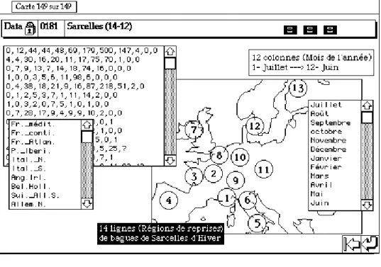
Create a data folder and go to the ADE-4•Data selection card. Select «Sarcelles» in the right-hand data menu. The corresponding card shows up as follows:

Table 1 Bird count data set.

07 08 09 10 11 12 01 02 03 04 05 06 1 0 12 44 44 48 69 179 500 147 4 0 0 1047 2 4 4 30 16 20 11 17 75 70 1 0 0 248 3 0 7 9 13 7 14 18 74 16 0 0 0 158 4 1 0 0 3 5 6 11 98 6 0 0 0 130 5 0 4 38 18 21 9 16 87 218 51 2 0 464 6 0 1 2 5 3 7 1 11 14 2 0 0 46 7 1 0 3 2 0 7 5 1 0 1 0 0 20 8 0 7 28 17 9 4 9 9 10 2 0 0 95 9 0 4 8 12 2 3 5 5 1 0 0 1 41 10 1 12 20 13 9 2 0 0 2 1 0 0 60 11 1 43 31 7 2 1 1 1 4 5 0 1 97 12 4 68 53 15 3 0 0 0 0 5 25 7 180 13 0 14 3 0 0 0 0 0 0 0 7 1 25 14 3 184 105 34 5 0 0 0 0 11 83 13 438 15 360 374 199 134 133 262 861 488 83 117 23 3049

(3)

Copy the data as usual. The three following files should be copied: Sar.edit,

Code_Mois3 and Code-Reg.

Sar.edit contents the number of returned rings in each location for the 12 months

sampling period (Table 1, numbers in italic indicate therow and column totals).

Code_Mois3 contents the names of the sampling months.

Code-Reg contents the names of the regions where the samples were taken.

2 - Definition of the geographical space

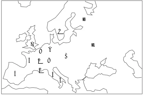
Use Copy files from the Data Folder menu to copy files Sarcelles_Carto and

Sarcelles_Digi (Fig. 1). These two files have a PICT format and must remain in

PICT format to be used by ADE modules.

4 1 2 3 5 6 7 8 9 A B C D E

Figure 1 Content of file Sarcelles_Digi. Characters (1,2...E) on the geographical map locate the center of the sampling regions.

Use the Digitalize option of the Digit module to create the file that contains the spatial coordinates of each site as follows (see section -2.2 for more details):

(4)

Choose the file Sarcelles_Digi as background map and type in SXY into the

Output XY file box (i.e., file that contains the spatial coordinates).

The output file has 14 rows (sites) and 2 columns. Open it to verify its content:

Input file: SXY Row: 14 Col: 2 1 | 87.0000 | 55.0000 | 2 | 84.0000 | 75.0000 | 3 | 63.0000 | 77.0000 | 4 | 31.0000 | 47.0000 | 5 | 116.0000 | 45.0000 | 6 | 133.0000 | 31.0000 | 7 | 68.0000 |113.0000 | 8 | 87.0000 | 98.0000 | 9 | 107.0000 | 77.0000 | 10 | 109.0000 |102.0000 | 11 | 146.0000 | 87.0000 | 12 | 130.0000 |143.0000 | 13 | 185.0000 |169.0000 | 14 | 206.0000 |111.0000 |

Values are given in pixels.

3 - Correspondence analysis

3.1 - The mathematical principle

Initially proposed by Hirschfeld (1935)4_{, and though long neglected (Hill, 1974)}5_,

correspondence analysis is a very widely used ordination technique (e.g., Greenacre and Vrba, 1984)6_{. Furthermore, Thioulouse and Chessel (1992)}7_{have described its joint}

property of reciprocal averaging (Hill, 1973)8_{and dual scaling. Williams (1952)}9

underscored that correspondence analysis was a mean of measuring a correlation within a contingency table (see volume 4).

Let L=[n_ij] be a table having I rows (sampling units) and J columns (species). Let

n_ij, for 1≤i ≤I and 1≤ j≤J , be the abundance of the jth species in the ith sampling

unit. Moreover, let n_i. = n_ij

j=1 J

∑

, n_.j = n_ij i=1 I

∑

, and n_..= n_i. i=1 I

∑

= n_{. j} j=1 J

∑

be, respectively, the row totals, the column totals, and the grand total.

Table P =[pij] of relative frequencies has I rows (sampling units) and J columns

(species) with p_ij being the proportion of the cell n_ij as follows:

p_ij= nij

n_.. for 1≤i≤I and 1≤ j ≤J

The row and column weights are respectively denoted by p_i.=ni.

n_.. and p.j = n_{. j} n_.. . Let

D_I =Diag p

(

_1., , p_i., , p_{I .}

)

and D_J =Diag p

(

_.1, , p_{. j}, p_.J

)

be respectively the diagonal matrices of row weights and column weights. Let x be a vector ( I

(5)

components) associated with the sampling units of L and let y be a vector ( J components) associated with the species of L .

Let X=

[ ]

x_ij =D-1_I PD-1_J −1_IJ with x_ij being a value as follows:

x_ij = pij p_i.p_{. j} −

1

Let define u₁ (first principal axis) as a vector in Rp solution of the equation

XtD_IXD_Ju₁ = u₁ with u₁tD_Ju₁ =1

with (first eigenvalue) being maximum. The first row scores in Rp are derived from this equation and are equal to R=X D_pu₁. This procedure is symmetric (duality) and one can define v₁ (first principal component) as a vector in Rn solution of the equation

XD_pXtD_nv₁ = v₁ with v₁tD_nv₁ =1

with (first eigenvalue) being maximum. The corresponding first column scores in Rn are equal to C=XtD_nv₁.

3.2 - Computation

Transform the Sar.edit file into a binary file (Sar) using the Text->Binary option of the TextToBin module. Select COA popmenu of the ADE•Base selection menu and

Run the module:

The eigenvalues, the inertia ratio of each axis, and the cumulated inertia shows up as follows:

(6)

Save the listing to store information about the results of this computation:

fc/COA: Correspondance analysis Input file: Sar

Number of rows: 14, columns: 12

File Sar.fcpl contains the edge distribution of rows It has 14 rows and 1 column

File Sar.fcpc contains the edge distribution of columns It has 12 rows and 1 column

File Sar.fcta contains the doubly centred table DI-1*P*DJ-1 -1I*1J' It has 14 rows and 12 columns

File Sar.fcma contains: the number of rows: 14 the number of columns: 12 the total number: 3049

---DiagoRC: General program for two diagonal inner product analysis Input file: Sar.fcta

--- Number of rows: 14, columns: 12

---Total inertia: 1.02898

---Num. Eigenval. R.Iner. R.Sum |---Num. Eigenval. R.Iner. R.Sum | 01 +6.6759E-01 +0.6488 +0.6488 |02 +2.0547E-01 +0.1997 +0.8485 | 03 +7.8334E-02 +0.0761 +0.9246 |04 +2.5641E-02 +0.0249 +0.9495 | 05 +1.8508E-02 +0.0180 +0.9675 |06 +1.3187E-02 +0.0128 +0.9803 | 07 +9.6811E-03 +0.0094 +0.9897 |08 +6.1038E-03 +0.0059 +0.9957 | 09 +3.2126E-03 +0.0031 +0.9988 |10 +8.7743E-04 +0.0009 +0.9996 | 11 +3.8148E-04 +0.0004 +1.0000 |12 +0.0000E+00 +0.0000 +1.0000 | File Sar.fcvp contains the eigenvalues and relative inertia for each axis

--- It has 12 rows and 2 columns

File Sar.fcco contains the column scores --- It has 12 rows and 3 columns

File :Sar.fcco Minimum/Maximum

---Col.: 1 Mini = -1.72343 Maxi = 0.661126

Col.: 2 Mini = -0.428492 Maxi = 1.265

Col.: 3 Mini = -0.571144 Maxi = 0.68004

File Sar.fcli contains the row scores --- It has 14 rows and 3 columns

File :Sar.fcli Minimum/Maximum

(7)

Col.: 2 Mini = -0.612134 Maxi = 0.958164

Col.: 3 Mini = -1.00423 Maxi = 0.81009

---The file SAR.fcta contains the values [p_ij/(p_i.*p_.j)]-1 which measure the distance between the observed frequency in the ith region i for the jth month and the expected frequency given by the independence model between the variables "space" (rows) and "time" (columns). These values are computed as follows: [(a_ij*a_..)/(a_i.*a_.j)] - 1 where a_ij is the observed value, a_i. the row totals, a_.j the column totals, a_.. the total number of recaptured Teals (3049). For instance, (12*3049)/(1047*360) - 1 = -0.903 (row 1 and column 2). You can edit the file SAR.fcta to verify its contents:

Input file: Sar.fcta Row: 14 Col: 12 1 | -1.0000 | -0.9029 | -0.6574 | -0.3561 | 0.0432 | 0.5108 | 0.9896 | 0.6911 | -0.1228 | -0.8597 | -1.0000 | -1.0000 | 2 | 2.2785 | -0.8634 | -0.0138 | -0.0115 | 0.8350 | 0.0168 | -0.2023 | 0.0709 | 0.7635 | -0.8519 | -1.0000 | -1.0000 | 3 | -1.0000 | -0.6248 | -0.5356 | 0.2606 | 0.0081 | 1.0313 | 0.3258 | 0.6586 | -0.3673 | -1.0000 | -1.0000 | -1.0000 | 4 | 0.5636 | -1.0000 | -1.0000 | -0.6464 | -0.1249 | 0.0581 | -0.0153 | 1.6695 | -0.7116 | -1.0000 | -1.0000 | -1.0000 | 5 | -1.0000 | -0.9270 | -0.3323 | -0.4056 | 0.0298 | -0.5553 | -0.5987 | -0.3360 | 1.9355 | 3.0377 | -0.8877 | -1.0000 | 6 | -1.0000 | -0.8159 | -0.6455 | 0.6654 | 0.4839 | 2.4886 | -0.7470 | -0.1532 | 0.9016 | 0.5972 | -1.0000 | -1.0000 | 7 | 9.1633 | -1.0000 | 0.2229 | 0.5322 | -1.0000 | 7.0237 | 1.9094 | -0.8229 | -1.0000 | 0.8367 | -1.0000 | -1.0000 | 8 | -1.0000 | -0.3759 | 1.4028 | 1.7418 | 1.1556 | -0.0347 | 0.1025 | -0.6645 | -0.3423 | -0.2266 | -1.0000 | -1.0000 | 9 | -1.0000 | -0.1737 | 0.5907 | 3.4844 | 0.1099 | 0.6774 | 0.4192 | -0.5681 | -0.8476 | -1.0000 | -1.0000 | 2.2333 | 10 | 2.3878 | 0.6939 | 1.7175 | 2.3197 | 2.4131 | -0.2358 | -1.0000 | -1.0000 | -0.7917 | -0.3878 | -1.0000 | -1.0000 | 11 | 1.0955 | 2.7545 | 1.6054 | 0.1057 | -0.5309 | -0.7637 | -0.8800 | -0.9635 | -0.7424 | 0.8936 | -1.0000 | 0.3667 | 12 | 3.5170 | 2.1996 | 1.4004 | 0.2768 | -0.6208 | -1.0000 | -1.0000 | -1.0000 | -1.0000 | 0.0204 | 2.6194 | 4.1553 | 13 | -1.0000 | 3.7429 | -0.0217 | -1.0000 | -1.0000 | -1.0000 | -1.0000 | -1.0000 | -1.0000 | -1.0000 | 6.2968 | 4.3026 | 14 | 0.3922 | 2.5579 | 0.9543 | 0.1893 | -0.7403 | -1.0000 | -1.0000 | -1.0000 | -1.0000 | -0.0774 | 3.9383 | 2.9346 |

The two files SAR.fcpl and SAR.fcpc are the rows frequencies used as rows weights and the columns frequencies used as columns weights respectively (i.e., 1047/3049=0.3434 and 15/3049=0.0049):

---

---Input file: Sar.fcpl Input file: Sar.fcpc

Row: 14 Col: 1 Row: 12 Col: 1

1 | 0.3434 | 1 | 0.0049 | 2 | 0.0813 | 2 | 0.1181 | 3 | 0.0518 | 3 | 0.1227 | 4 | 0.0426 | 4 | 0.0653 | 5 | 0.1522 | 5 | 0.0439 | 6 | 0.0151 | 6 | 0.0436 | 7 | 0.0066 | 7 | 0.0859 | 8 | 0.0312 | 8 | 0.2824 | 9 | 0.0134 | 9 | 0.1601 | 10 | 0.0197 | 10 | 0.0272 |

(8)

11 | 0.0318 | 11 | 0.0384 |

12 | 0.0590 | 12 | 0.0075 |

13 | 0.0082 |

14 | 0.1437 |

---File SAR.fcvp contains the eigenvalues and relative inertia for each axis:

---Input file: Sar.fcvp

Row: 12 Col: 2 1 | 0.6676 | 0.6488 | 2 | 0.2055 | 0.1997 | 3 | 0.0783 | 0.0761 | 4 | 0.0256 | 0.0249 | 5 | 0.0185 | 0.0180 | 6 | 0.0132 | 0.0128 | 7 | 0.0097 | 0.0094 | 8 | 0.0061 | 0.0059 | 9 | 0.0032 | 0.0031 | 10 | 0.0009 | 0.0009 | 11 | 0.0004 | 0.0004 | 12 | 0.0000 | 0.0000 |

---The first column of this file is used to plot the eigenvalues graph. Note that the three first axes take into account 92.5 % of the total inertia of the table. Files SAR.fcco and

SAR.fcli contain the column scores and the row scores respectively. They can be used

to draw factorial maps.

The inertia analysis allows to add statistical aid in the interpretation of data (see section-2.2 for more details concerning the significance of the resulting values). Use

DDUtil and choose the Rows: Inertia analysis option to compute the row contributions

as follows:

Input file: Sar.fcta

Number of rows: 14, columns: 12

Inertia: Two diagonal norm inertia analysis Total inertia: 1.02898 - Number of axes: 3

File Sar.fccl contains the contribution of rows to the trace It has 14 rows and 1 column

Row inertia

All contributions are in 1/10000

---Absolute contributions---|Num |Fac 1|Fac 2|Fac 3|

| 1| 1824| 1593| 141| | 2| 160| 171| 247| | 3| 158| 311| 29| | 4| 344| 777| 456| | 5| 338| 6799| 478| | 6| 38| 92| 75|

(9)

| 7| 6| 40| 543| | 8| 13| 17| 2317| | 9| 8| 30| 1231| | 10| 119| 12| 2533| | 11| 541| 21| 468| | 12| 1591| 10| 8| | 13| 382| 34| 686| | 14| 4470| 85| 780| ---Relative

contributions---|Num |Fac 1|Fac 2|Fac 3||Remains| Weight | Cont.| | 1| 7686| 2066| 70|| 177 | 3433 | 1539 | | 2| 4286| 1409| 773|| 3530 | 813 | 243 | | 3| 5612| 3397| 124|| 865 | 518 | 182 | | 4| 4451| 3092| 691|| 1764 | 426 | 502 | | 5| 1356| 8381| 224|| 37 | 1521 | 1620 | | 6| 2514| 1839| 570|| 5075 | 150 | 100 | | 7| 186| 362| 1864|| 7586 | 65 | 221 | | 8| 417| 160| 8189|| 1232 | 311 | 215 | | 9| 375| 396| 6034|| 3193 | 134 | 155 | | 10| 2571| 84| 6403|| 941 | 196 | 301 | | 11| 6549| 79| 665|| 2706 | 318 | 536 | | 12| 9675| 19| 6|| 298 | 590 | 1067 | | 13| 7726| 217| 1628|| 427 | 81 | 321 | | 14| 9691| 56| 198|| 53 | 1436 | 2992 |

---In these tables, the column "Num" identifies the rows (14 sites) or the columns (12 months). The highest values of relative contributions are underlined to highlight the significance of factorial scores.

Choose the Columns: Inertia analysis option to compute the column contributions as follows:

Column inertia

All contributions are in 1/10000

---Absolute contributions---|Num |Fac 1|Fac 2|Fac 3|

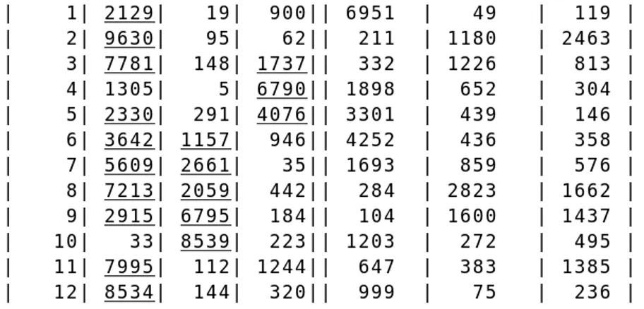
| 1| 39| 1| 141| | 2| 3656| 118| 201| | 3| 975| 60| 1855| | 4| 61| 0| 2717| | 5| 52| 21| 785| | 6| 201| 207| 445| | 7| 498| 767| 26| | 8| 1848| 1714| 967| | 9| 646| 4892| 347| | 10| 2| 2120| 145| | 11| 1707| 77| 2265| | 12| 310| 17| 99| ---Relative

(10)

| 1| 2129| 19| 900|| 6951 | 49 | 119 | | 2| 9630| 95| 62|| 211 | 1180 | 2463 | | 3| 7781| 148| 1737|| 332 | 1226 | 813 | | 4| 1305| 5| 6790|| 1898 | 652 | 304 | | 5| 2330| 291| 4076|| 3301 | 439 | 146 | | 6| 3642| 1157| 946|| 4252 | 436 | 358 | | 7| 5609| 2661| 35|| 1693 | 859 | 576 | | 8| 7213| 2059| 442|| 284 | 2823 | 1662 | | 9| 2915| 6795| 184|| 104 | 1600 | 1437 | | 10| 33| 8539| 223|| 1203 | 272 | 495 | | 11| 7995| 112| 1244|| 647 | 383 | 1385 | | 12| 8534| 144| 320|| 999 | 75 | 236 |

---4 - Data cartography

Use the Maps module with the Values option to plot the scores on the geographic map already prepared:

Use the file Sarcelles-carto as Background map (Pict file), SXY as XY file,

Code_mois3 as Label file and Sar as Input data file. If necessary, modify the G value

(Min & Max. selection in the Windows menu) to obtain the desired diameter of circles. This results in Fig. 2.

(11)

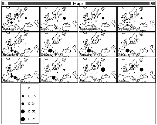
In this representation, the circle size is calibrated from the maximum value. Consequently, it is more relevant to draw the frequencies distributions per date (data in percentage per column). Threfore, you can transform file Sar into a file containing frequencies distributions per date (SarPCC).

Figure 3 Cartography of the frequency distributions of teals at each sampling date (data from SarPCC).

Use the Bin->Bin module with the Frequencies option. Choose Sar as Input file and type SarPCC as Output file and click the hand icon. Choose option 2:

Input file: Sar

(12)

---Transformation X -> X / column sum ---Output file: SarPCC

Run again the Maps module (Values option) and use SarPCC as Input data file.

This results in Fig. 3.

These graphs show the dispersion of teals according to the season: a wide spatial distribution in summering periods (July-September and May-June) and a decrease in distribution during wintering periods (gregariousness from December to March) after the automn migration. The migration loop occurs as follows: teals start from their summering areas to wintering areas through the north of Europe and come back by the south of Europe. 4 1 2 3 5 6 7 8 9 10 11 12 13 14 A B C D E

(13)

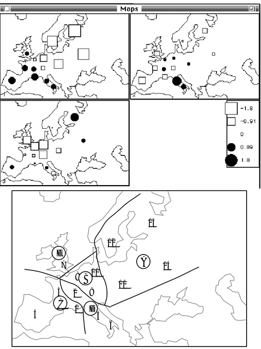
5 - Cartography of factorial scores

Spatio-temporal correspondences can be shown by ploting the factorial scores on each axis on the geographic map. Use again the Maps module (Values option) and use

Sar.fcli as Input data file:

This results in the following graph which leads to the partition of the studied area into five zones (Fig. 4).

6 - Plotting circular data (see Graph1D : Stars)

Use the Bin->Bin module (Frequencies option) to obtain the frequencies distributions by row. Choose Sar as Input file and SarPCR as Output file, and the first option.

Go to the ADE•Old selection card and select the CircleChart Basic program. Fill in the dialog boxes as follows:

(14)

Min= 0 Max= .8

1 2 3 4 5

6 7 8 9 10

11 12 13 14

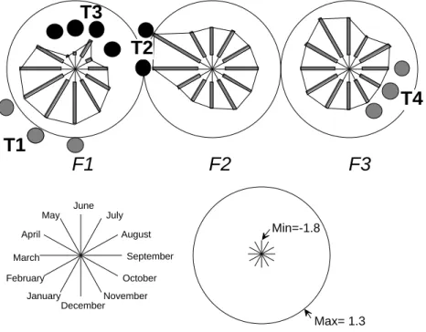
Figure 5 Circle diagram of the percentages of recaptures per month for each site. The circles are divided into 12 parts and the length of the thick grey lines is proportional to the percentages of recaptures Min=-1.8 Max= 1.3

T3

T1

T2

T4

F1

F2

F3

January February March April May December November October September August July June

(15)

This results in Fig. 5 that depicts the percentage of recaptures per month for each site (1 to 14).

Drawing the values of the factorial scores with the same module gives a synthethic wiew of the spatial and temporal patterns of teals distribution and migrations (Fig. 6).

The first axis defines two periods: July-September, May-June, and November-March which correspond to two zones (1 to 6 and 10 to 14) associated with summering and wintering periods respectively.

The second axis separates the wintering period in two components: a wintering period (December-February in Camargue, western France and Spain) and a spring migration (displacement towards eastern France and Italia in March-April).

The third axis describes the migration towards Switzerland, Germany, Benelux and British Iles in autumn.

7 - Table reorganization (see FilesUtil)

The previous results about the spatial and temporal patterns of teals distribution have shown that it is possible to distinguish four periods and five zones among the teal recaptures. Original raw data can be rewritten according to this partition by summing several rows and several columns. Go to the ADE•Old selection card and select the

RowOrganise Quickbasic program, which allows to sum up or to duplicate row blocks

in a file. The program makes a loop whenever you decide to add rows. Fill the dialog boxes as follows to sum up rows:

(16)

Information about this computation are given in the following listing:

File Sar is binary

Number of rows = 14 Number of columns = 12 Row 1 of Sar1 contains the sum or rows of Sar from selection 11a14 with 4 rows

Row 2 of Sar1 contains the sum or rows of Sar from selection 8a10 with 3 rows

Row 3 of Sar1 contains the sum or rows of Sar from selection 1;3;4 with 3 rows

Row 4 of Sar1 contains the sum or rows of Sar from selection 2;5;6 with 3 rows

Row 5 of Sar1 contains the sum or rows of Sar from selection 7 with 1 rows

(17)

Number of rows = 5 Number of columns = 12

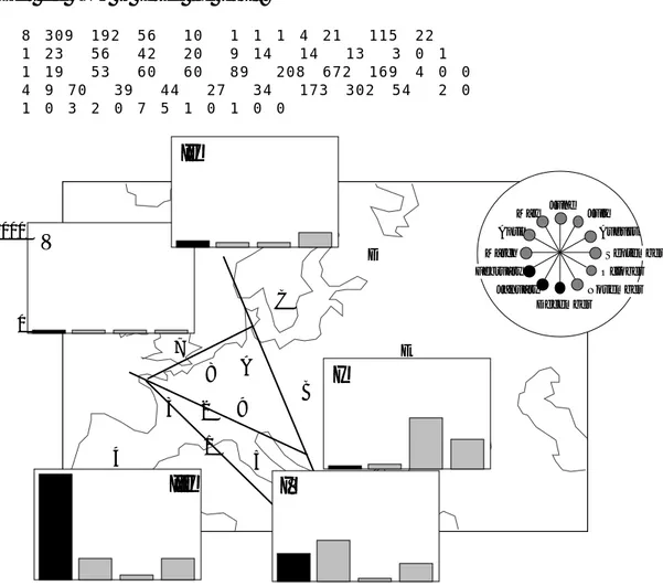
Edit file Sar1 to verify the result:

8 309 192 56 10 1 1 1 4 21 115 22 1 23 56 42 20 9 14 14 13 3 0 1 1 19 53 60 60 89 208 672 169 4 0 0 4 9 70 39 44 27 34 173 302 54 2 0 1 0 3 2 0 7 5 1 0 1 0 0 4 1 2 3 5 6 7 8 9 A B C D E 0 1000 January February March April May December November October September August July June

V

I

III

II

IV

Figure 7 Synthetic diagrams of teal recapture. Histograms use the values resulting from the rearrangement of raw data.

Run the ColOrganise Quickbasic program to sum up columns:

File Sar1 is binary

Column 1 of Sar2 contains the sum or Columns of Sar1 from selection 6a8 with 3 Columns

Column 3 of Sar2 contains the sum or Columns of Sar1 from selection 1a2;11a12 with 4 Columns

(18)

File Sar2 is binary

File Sar2 contains the followings values:

3 25 454 258

37 16 25 118

969 173 20 173

234 356 15 153

13 1 1 5

Finally, recapture count data (Table 1) can be summarized by Fig. 7.

Références

1_{Hoffmann, L. (1960) Untersuchungen an Enten in der Camargue. Ornithologische}

Beobatcher : 57, 35-50.

2_{Lebreton, J.D. (1973) Etude des déplacements saisonniers des Sarcelles d'hiver, Anas}

c. crecca L., hivernant en Camargue à l'aide de l'analyse factorielle des

correspondances. Compte rendu hebdomadaire des séances de l'Académie des sciences. Paris, D : III, 277, 2417-2420.

3_{Auda, Y., Chessel, D. & Tamisier, A. (1983) La dispersion spatiale des Oiseaux au}

cours du cycle annuel : deux méthodes de description graphique. Compte rendu

hebdomadaire des séances de l'Académie des sciences. Paris, D : III, 297, 387-392.

4_{Hirschfeld, H.O. (1935) A connection between correlation and contingency.}

Proceedings of the Cambridge Philosophical Society, Mathematical and Physical Sciences : 31, 520-524.

5_{Hill, M.O. (1974) Correspondence analysis : A neglected multivariate method. Journal}

of the Royal Statistical Society, C : 23, 340-354.

6_{Greenacre, M.J. & Vrba, E.S. (1984) Graphical display and interpretation of antelope}

census data in African wildlife areas, using correspondence analysis. Ecology : 65, 984-997.

7_{Thioulouse, J. & Chessel, D. (1992) A method for reciprocal scaling of species}

tolerance and sample diversity. Ecology : 73, 670-680.

8_{Hill, M.O. (1973) Reciprocal averaging : an eigenvector method of ordination. Journal}

of Ecology : 61, 237-249.

9_{Williams, E.J. (1952) Use of scores for the analysis of association in contingency}

Correspondence analysis

ADE-4