Lire
4.1 Motivations and Objectives
The use of two or more GNSS constellations and two frequencies in GAST-F produces several benefits, in terms of accuracy, integrity monitoring and system continuity. Despite the advantages in obtaining a larger number of measurements, there is at least one possible problem to cope with: the limited number of channels present in a GNSS receiver. The use of single frequency single constellation GBAS implies the tracking of up to 10-12 satellites. Considering the presence of a second constellation, this number can be doubled. It can be seen in the remainder of the chapter that 22 satellites may be visible at the same time, under defined circumstances, and this number must be also doubled if a second frequency is used. It is clear that any receiver, to work in dual constellation and dual frequency, need more than 44 channels to be sure that all satellites in view are tracked.
The problem of the number of visible satellites is, however, not only related to the number of channels in a receiver. In GBAS, another issue is represented by the maximum number of corrections that could be broadcasted through the VDB link. The correction message, as currently structured in GBAS GAST D, limits the number of corrections to 18. Considering the optimization of the message occupation, this number may increase to 27 (SESAR 15.3.7; WP3), which is considered as sufficient for GAST D. Considering the development of GAST F that uses a processing mode different from GAST D, and in order to maintain interoperability between the two GBAS services, the ground station must broadcast corrections for both GAST-D and F. Under these circumstances, the limit stated before must be split almost by two, even if, considering the redundancy of certain information present in the correction message, some space could be saved. Considering a possible limit of 15 corrections, there is a need to have a satellite selection algorithm in order to avoid accuracy problem when all satellites in view cannot be used.
Over the years, many methods were proposed to select a satellite subset instead of using all satellites in view in order to solve problems cited before. The choice of a satellite subset was focused on the search of the best subset in order to preserve the accuracy. The main parameter on which the search was focused on, was the DOP, also VDOP and HDOP, because it is the only index relating the accuracy to the constellation geometry.
4.2 Satellite Selection Methods
The algorithms presented in the next section were developed for the case of a subset having no more than four or five satellites. Their use to search a subset composed by a bigger number leads to an increase of the computational load in some cases, or to a non-optimal subset choice.
4-SATELLITE SELECTION
4.2.1 Optimal Solution
One of the main selection algorithms proposed in the past, is the optimal solution (Liu, et al., 2009). This algorithm computes the best value of GDOP trying all the possible satellite subset at the cost of a great computational load with the growth of the number of satellites in view. For example with 18 visible satellites and the search for a 12-satellite subset, the algorithm has to compute 18564 different GDOP values, the total amount being given by the following formula:
𝐶1218= 18!
12! (18 − 12)!= 18564
Using a 20-satellite subset out of 40 visible, the number increases to 1.38 ∙ 1011. It can thus be
understood that this method works properly only for single constellation, when a low number of satellites is in view and a small satellite subset is searched for. Note that it is possible to use the same type of algorithm to optimize other DOP values, such as PDOP, HDOP or VDOP; also the protection level can be used as the optimization criterion.
4.2.2 Modified Minimum GDOP
An alternative method is the Modified Minimum GDOP. In this algorithm the first chosen satellite of the subset is the one with the highest elevation angle and the other satellites are searched as in the “optimal solution” case (Cryan, et al., 1992). This method reduces the computational burden in comparison with the “optimal solution” but the number of all possible combinations to be analysed can be still prohibitively large. Using the same example used for the optimal solution, 18 satellites available and a 12 satellites subset, and choosing the first as the one with the higher elevation angle the total amount of possible combination to be considered is 12376 and is given by:
𝐶1117 = 17!
11!(17−11)!= 12376
It can be seen that the number of combinations to be analyzed is still very large.
4.2.3 Lear’s Simple Satellite Selection
This technique, shown in (Cryan, et al., 1992), follows a defined procedure to choose the first three satellites and the last one is chosen minimizing the DOP value. The procedure works in the following manner:
The first satellite is chosen finding the one with the highest elevation angle.
The second is the one having an angle between the LOS (Line Of Sight) of the selected satellite and the LOS of the first satellite as close as possible to 90°.
The third satellite chosen is the one that has the LOS perpendicular to the plane formed by the two previous satellites chosen.
The last satellite is chosen to minimize the GDOP (Cryan, et al., 1992).
This technique has almost no computational load compared to the two previous methodologies. The main drawback of this method is that it was developed only for a four satellites subset and this is not enough for GBAS, even for single constellation and single frequency GBAS.
4.2.4 Fast Satellite Selection Algorithm
The main problem of the previous techniques is that they were developed to work better, in some cases to work only, with a 4 satellite subset and a limited number of satellites in view. When a larger number of satellites in the subset is searched, and there are a lot of satellites in view, the computational burden increases rapidly. Considering the scope of this analysis and the development of dual constellation dual frequency GBAS service, the number of satellites for the subset can be larger than ten. In order to overcome the problem of finding a subset with more than ten satellites without increasing too much the computational load, new algorithms were developed and are presented in the following.
The algorithm proposed in (Zhang, et al., 2008) is a good solution to the problem related with a subset bigger than 4 satellites. In this technique, a preliminary study with a simulated constellation was used to find the subset geometry with the best GDOP value starting from 4 and up to 15 satellites. From the result analysis, it is possible to see how the best GDOP varies according to the number of satellites selected at the zenith or near (> 80°) it and selecting the remaining according to their azimuth in order to have a homogenous distribution.
4-SATELLITE SELECTION
Table 14 – GDOP values for different number of satellite at high elevation for a simulated study (Zhang, et al., 2008)
NUMBER OF SV AT THE ZENITH
1 2 3 4 5 6 7 SA TE LL ITE SU B SE T 4 3.3528 5 2.8169 2.7482 6 2.4953 2.2123 2.5466 7 2.281 1.8907 2.0108 2.4459 8 2.1279 1.6764 1.6892 1.91 2.3854 9 2.013 1.5233 1.4749 1.5884 1.8495 2.3451 10 1.9237 1.4084 1.3217 1.3741 1.528 1.8092 2.3163 11 1.8523 1.3191 1.2069 1.221 1.3136 1.4877 1.7804 12 1.7938 1.2477 1.1176 1.1061 1.1605 1.2733 1.4589 13 1.7451 1.1892 1.0461 1.0168 1.0457 1.1202 1.2445 14 1.7039 1.1405 0.9877 0.9454 0.9564 1.0054 1.0914 15 1.6685 1.0993 0.939 0.8869 0.8849 0.9161 0.9766 16 1.6379 1.0639 0.8977 0.8382 0.8265 0.8446 0.8873
The values of the GDOP shown in Table 14 are computed for a simulated constellation placing satellites at high elevation angle and the remaining equally spaced at low elevation angle. This study permits to establish how many satellites must be selected between the ones with the higher elevation angle before selecting the remaining ones following a defined algorithm.
The algorithm works in 4 steps:
1. Computation of the elevation and azimuth angle of all visible satellites.
2. According to the number of satellites of the subset, 𝑛, the number of satellites with the highest elevation angle is selected. Defined p=number of satellite at zenith; to find the p satellites with the highest elevation.
3. To divide the sky in 𝐾 = 𝑛 − 𝑝 equally-spaced in azimuth portions and group the satellites in each portions. It is possible to start the sky division from one particular direction or to select one satellite as reference and start from its azimuth. The satellite with the lowest elevation angle must be found and noted as 𝑆𝑝+1, it can be removed or used as reference for the group
subdivision.
4. The fourth step is to combine one satellite from each 𝑘𝑡ℎ group with the others chosen in the
possible subset has to be done, the satellites that belong to the subset with minimum GDOP are selected for the solution computation. The total number of subset is:
𝑇 = 𝐶1× 𝐶2× … × 𝐶𝑛−𝑝 Eq. 4.1
Where:
𝐶𝑘is the number of satellites in the 𝑘𝑡ℎ group.
In Figure 51 an example of sky plot subdivision with high elevation angle satellites noted in green and the remaining satellites sort in groups. The satellite with the lowest elevation angle is coloured in red, it can be removed from the subsets or used as starting point of the groups subdivision.
Figure 51 – Fast satellite selection sky subdivision example (Zhang, et al., 2008)
4.3 Selected Methods for Simulation
Considering the methods found in literature and the conditions of DF/DC GBAS, all methods developed to work properly for searching four or five satellites presented in section 4.2.1, 4.2.2 and 4.2.3 are not considered due to the high computational burden. However, the Optimal Solution method will be used to find the real best DOP value or protection level and to compare it with the other selection methods.
4-SATELLITE SELECTION
of other analyzed methods. The selection algorithm proposed in 4.2.4 is used to find the best subset due to its ability to find it without increasing too much the computational load. A last methods, even if is not a satellite selection algorithm is the selection of the n satellites with the highest elevation angle. To summarize the selection algorithms or methods used for simulation are:
Fast Satellite Selection; In order to make the algorithm faster, instead of computing the DOP for each combination, the satellite with the lower elevation angle will be systematically selected in each bin along with the satellites with high elevation angle.
Maximum Elevation Angle; even if this is not an algorithm and it has not been presented before it will be used for its simplicity. The advantage of this method is to completely cancel the computational load. In this case, only the 𝑛 highest elevation satellites are kept. The choice of the higher elevation satellites is determined by the analysis of the GAD and AAD model and as well as by the impact of the ionospheric delay and multipath on low elevation satellites. Analysing the GAD and AAD model, it is possible to see that the standard deviation of the residual errors is smaller for the satellite with higher elevation angle. The residual uncertainty of the tropospheric and ionospheric delay also shows a relationship between elevation angle and standard deviation values: the higher the elevation, the lower the standard deviation.
Brute Force VPL (Optimal Solution); this is a modification of the optimal solution, where the optimization criteria is the VPL instead of the DOPs value. In the algorithm, a control also of the 𝑆𝑣𝑒𝑟𝑡 and 𝑆𝑣𝑒𝑟𝑡2 is done to be sure to find the lowest and valid protection level.
All the algorithms will be compared with the all-in-view condition to analyse also the accuracy loss or the protection level loss.
4.4 Simulations Baseline
In order to evaluate the impact in using a satellites subset instead of the whole set of satellites in view, a series of parameters have been computed across 18 airports for a simulated period of 10 days with 60 seconds resolution.
4.4.1 Airports Coordinates
Table 15 – Airports coordinates used in simulation
Airport Latitude (°) Longitude (°) Memphis 35.0424 -89.9767 Denver 39.8584 -104.667 Dallas 32.8964 -97.0376 Newark 40.6925 -74.1687 Washington 38.9445 -77.4558 Los Angeles 33.9425 -118.4081 Orlando 28.4289 -81.3160 Minneapolis 44.8805 -93.2169 Chicago 41.9796 -87.9045 Tacoma 47.1377 -122.4765 Anchorage 61.2167 -149.90 Bremen 53.0429 8.7808 Malaga 36.68 4.5124 Sydney -33.9636 151.1859 Amsterdam 52.30907 4.763385 Rio -22.8088 -43.2436 Peking 40.080109 116.584503 Johannesburg -26.139099 28.246000
4.4.2 DOP Analysis and Computational Load
The concept of DOP has been already presented in 0. For this analysis the VDOP and HDOP of the satellite subsets and of the all-in-view situation will be analyzed.
𝐻 = (𝐺𝑇∙ 𝐺)−1 Eq. 4.2
𝑉𝐷𝑂𝑃 = 𝐻3,3; 𝐻𝐷𝑂𝑃 = √𝐻1,12 + 𝐻
2,22 Eq. 4.3
A second type of parameter that helps to understand the computational load of each selection algorithm is the time spent to find the selected subset. The aim in analysing this parameters is just to have an index
4-SATELLITE SELECTION
of the computational load of each method, it is however not representative of a real time implementation in an aircraft embedded subsystem.
4.4.3 Protection Level Computation
The previous parameters are not dependent on the simulated processing mode but only on the subset’s satellite number. To take into account the possibility to use different processing modes, two subsections are present: GAST D and the I-Free processing mode. The parameters analyzed for each one are the Vertical Protection Level (VPL) and the Lateral Protection Level (LPL) computed as in (RTCA Inc.; DO253-C, 2008):
𝑉𝑃𝐿 = max{𝑉𝑃𝐿𝐻0; 𝑉𝑃𝐿𝐻1} Eq. 4.4
𝐿𝑃𝐿 = max {𝐻𝑃𝐿𝐻0; 𝐿𝑃𝐿𝐻1} Eq. 4.5
Details about the VPL and LPL are given in 2.3.3.2
Values of 𝜎𝑝𝑟 𝑔𝑛𝑑 are used according to results obtained in section 3.4
4.4.4 Geometry Screening Availability
The values of 𝑆𝑣𝑒𝑟𝑡 and 𝑆𝑣𝑒𝑟𝑡2 are also analyzed in order to simulate the impact of the subset on the
geometry screening monitor 5.1.2. Details about 𝑆𝑣𝑒𝑟𝑡 are given in 2.3.3.2.
max {𝑆𝑣𝑒𝑟𝑡} = max
i {𝑆3,𝑖+ 𝑆1,𝑖 𝑡𝑔(𝐺𝑃𝐴)} Eq. 4.6
𝑆𝑣𝑒𝑟𝑡2is the sum of the two biggest 𝑆𝑣𝑒𝑟𝑡. The two parameters have to not exceed a limit dependent on
the number of constellations used. The limit for a single constellation GBAS service is respectively 4 and 6. Considering the use of dual constellation in the simulations, they can be adapted to 2 and 3.
4.5 Simulation Results
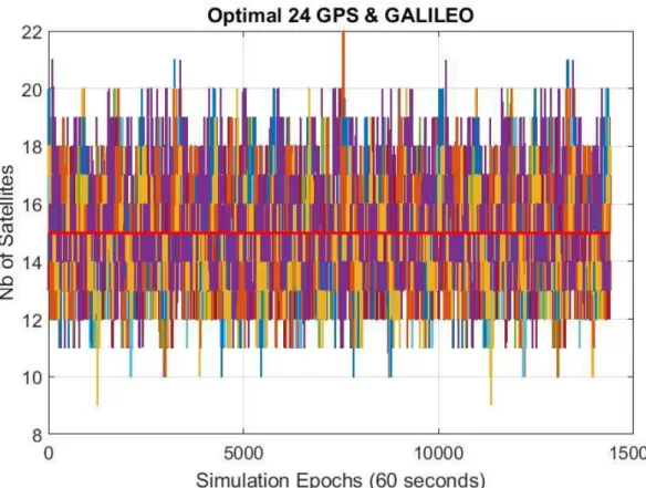
4.5.1 Dual Constellation 12 Satellite subset
In this simulation, a dual constellation composed by the optimal 24 GPS and the optimal 24 Galileo constellations is simulated because these two constellations represent the baseline for the GAST-F service. The next figure shows the number of visible satellites across all the epochs and airports.
Figure 52 – Number of Satellites for all the simulated epochs and airports and 12 satellites subset in red
4-SATELLITE SELECTION
It is possible to see in the previous figures that for more than 92% of epochs, there are more satellites than the subset limit across all airport. Under this condition, the parameters computed for the all-in-view case and the ones computed using only a subset may be quite different. The computational load, due to a difference of 10 satellites in rare case between satellites in view and subset, is expected to be very high.
4.5.1.1 Impact of the Selection Method on the DOP Value
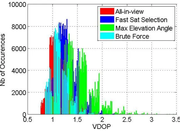
The values of the DOP, in the vertical and horizontal domain, provide a feedback about the accuracy that the all-in-view and the three selection algorithms are able to provide according to the number of satellite and their geometry in the sky. In Figure 54 and Figure 55 the values of VDOP and HDOP are shown.
Table 16 – VDOP percentile at 95, 99 and 99.9 % for 12 satellites subset
95 % VDOP 99 % VDOP 99.9% VDOP
All-in-view 1.4115 1.6099 1.9041
Fast Satellite Selection 1.6208 1.8551 2.1710
Maximum Elevation Angle 2.0411 2.4575 3.0718
Brute Force 1.4236 1.6180 1.9103
Figure 55 – HDOP values across all epochs and airports for all the methods and for all-in-view satellites Table 17 – HDOP percentile at 95, 99 and 99.9 % for 12 satellites subset
95 % HDOP 99 % HDOP 99.9% HDOP
All-in-view 0.8758 0.9770 1.1125
Fast Satellite Selection 0.9760 1.0675 1.2383
Maximum Elevation Angle 1.0274 1.1182 1.3037
4-SATELLITE SELECTION
It is possible to see from the analysis of Figure 54, Figure 55, Table 16and Table 17 that, using a satellite subset, the DOP values are higher than for the all-in-view case. In particular, for the maximum elevation angle selection method, the VDOP values are clearly bigger than the other methods. The fast satellite selection and the brute force are able to provide values similar in magnitude to the all-in-view solution, the brute force methods seems in any case to provide slightly better results than the fast selection criteria. In the next table, the average time to compute the previous parameters for one airport will be listed for all the three methods. The maximum time for each method will be listed as well in Table 18. This analysis aims to provide an insight of the computational load of each method.
Table 18 – Computational time, in seconds, for all methods with 12 satellites subset
All-in-View Fast Satellite Selection
Max Elevation
Angle Brute Force
Maximum Time 0.0604 0.1668 0.0537 119.14
Average Time 6.3702 ∗ 10−4 1.5 ∗ 10−3 3.2416 ∗ 10−4 0.8096
The brute force selection criteria is, as expected, the one with the highest computational load due to the number of combinations that has to be analyzed in order to find the best VPL. The other selection criteria require a computation time similar to the all-in-view case where no selection is done.
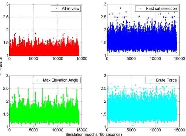
4.5.1.2 GAST D Protection Level
The simulated processing mode is the one used in GAST D, the sigma values for this service type are computed considering the model proposed in (RTCA Inc. DO245-A) and in (RTCA Inc.; DO253-C, 2008).
the non-aircraft RMS error is computed considering results obtained in Table 10 and divided by √4 to consider the presence of four reference receivers at ground
the airborne pseudorange performance are computed using the AAD model considering a B level (2.3.3), then it is multiplied by a factor of 1.3 in order to take into account the increased noise level related to the use of 30 seconds as smoothing constant instead of 100 seconds (Murphy, et al., 2010).
the RMS of the aircraft multipath is computed as in the model given in Eq. 2.69
the ionospheric and the tropospheric Residual Error are computed as in Eq. 2.70 and Eq. 2.52 𝐷𝑉and 𝐷𝐿, represent the difference in the vertical and lateral domain between the 30 seconds and the
𝑇ℎ(𝐷𝑉) = 𝐾𝑓𝑑𝐷√∑ 𝑆𝐴𝑝𝑟 𝑣𝑒𝑟𝑡,𝑖2 𝜎𝐷𝑅 2 𝑁 𝑖=1 Eq. 4.7 𝑇ℎ(𝐷𝐿) = 𝐾𝑓𝑑𝐷√∑ 𝑆𝐴𝑝𝑟 𝑙𝑎𝑡,𝑖2 𝜎 𝐷𝑅 2 𝑁 𝑖=1 Eq. 4.8 𝐾𝑓𝑑𝐷 , is the multiplier taking into account for the probability of false alarm. It is set at 5.5
considering a continuity risk of 4 × 10⁻⁸
𝜎𝐷𝑅 = 𝐹𝑃𝑃× 𝜎𝑣𝑖𝑔× 140 × 𝑉_𝑎𝑖𝑟; Considering a value of 𝜎𝑣𝑖𝑔= 4 𝑚𝑚/𝑘𝑚 and a landing speed of the aircraft of 72 𝑚/𝑠, the previous model can be approximated to 𝜎𝐷𝑅 = 𝐹𝑃𝑃× 0.04 𝑚
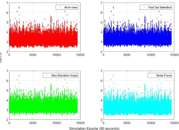
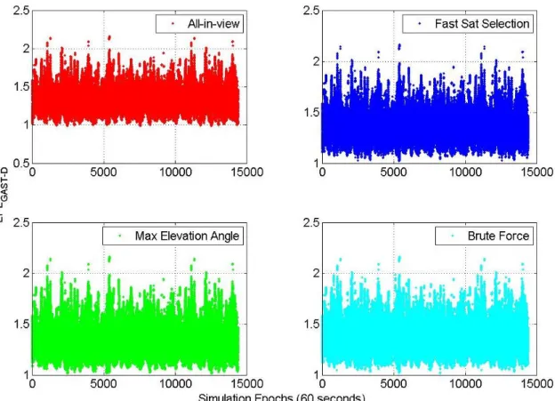
The next figures show the VPL and LPL as in Eq. 4.4 and Eq. 4.5 and the values of 𝑆𝑣𝑒𝑟𝑡 and 𝑆𝑣𝑒𝑟𝑡2.
The aim of these two plots is to verify that at any epoch, the limit value of 10 meters is not exceeded by VPL or LPL, or the 2 and 3 limits are not overcome by 𝑆𝑣𝑒𝑟𝑡 and 𝑆𝑣𝑒𝑟𝑡2.
4-SATELLITE SELECTION
Figure 57 – GAST-D LPL computed across all the epochs and airports for three selection methods and all-in-view satellites
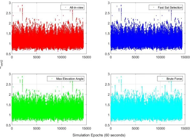
Figure 59 – GAST D 𝑆𝑣𝑒𝑟𝑡2 values across all epochs and airports for three methods and all-in-view satellites As expected, the VPL provides larger values than the LPL. In both figures, the protection levels do not overcome the 10 meters limit, making the GAST D service available at all airports and at all epochs. The brute force algorithm is optimized to find the lowest VPL. This explains why at several epochs, the LPLs found by the brute force algorithm is higher than the ones found by the other two methodologies.
Table 19 – Geometry screening availability for all the selection methods with 12 satellites and all in view case
VPL Availability LPL Availability 𝑺𝒗𝒆𝒓𝒕 Availability 𝑺𝒗𝒆𝒓𝒕𝟐 Availability All-in-view 100 % 100 % 100 % 100 % Fast Sat Selection 100 % 100 % 100 % >99.999 % Max Elevation Angle 100 % 100 % 99.92 % 99.79 % Brute Force 100 % 100 % 100 % 100 %
4-SATELLITE SELECTION
The comparison between the three selection methods shows that the brute force algorithm is able to find the lowest VPL, the fast satellite selection finds geometries providing VPL values slightly larger than the brute force. This last provides, indeed, some geometry screening unavailability due to the overcoming of the 𝑆𝑣𝑒𝑟𝑡2 limit of 3. The use of geometries based on the selection of the satellites with
the maximum elevation angle is the one providing the largest VPL values, moreover in several epochs the 𝑆𝑣𝑒𝑟𝑡 and 𝑆𝑣𝑒𝑟𝑡2 limits are overcome, making these epochs unavailable. In the horizontal domain the
use of the maximum elevation angle criteria provide better result than the other two methodologies, the results are however good for all the three selection criteria.
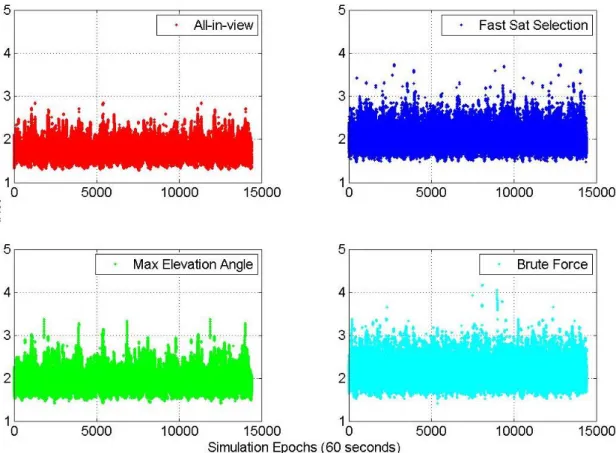
4.5.1.3 I-Free Protection Level
In the frame of dual constellation and dual frequency GBAS research, a possible candidate for the processing mode is the I-Free (2.2.2.2.3). This mode permits to remove entirely the ionospheric delay from the code measurement at the cost of increased noise level, at the ground for the computation of the pseudorange correction and at the airborne level for the final position computation. To compute the protection level considering the use of this technique, there are no official formula as for the GAST D service, so the computation of these parameters will be done considering the results obtained in the analysis of the performance for noise and multipath at ground station level for L1 and L5. It has to be reminded that a calibration issue has been found n L5 band measurements and that it impacts also the I-free results. All the components taking into account the ionospheric delay for the computation of the protection level in GAST D will be removed for the I-Free protection level. The divergence terms, 𝐷𝑉
and 𝐷𝐿, are set at zero because the double smoothing constant is not used in this case. The sigma ground
will be inflated considering the use of the two frequencies, as well as the sigma airborne. The total sigma is:
𝜎𝑡𝑜𝑡 𝐼−𝐹𝑟𝑒𝑒(𝑖) = √𝜎𝑝𝑟 𝑔𝑛𝑑 𝐼−𝐹𝑟𝑒𝑒,𝑖2 + 𝜎
𝑡𝑟𝑜𝑝𝑜,𝑖+ 𝜎𝑝𝑟 𝑎𝑖𝑟 𝐼−𝐹𝑟𝑒𝑒,𝑖2 Eq. 4.9
Where:
𝜎𝑝𝑟 𝑔𝑛𝑑 𝐼−𝐹𝑟𝑒𝑒 is defined using the bound defined in 3.4
𝜎𝑝𝑟 𝑎𝑖𝑟 𝐼−𝐹𝑟𝑒𝑒= √𝜎²𝑝𝑟 𝑎𝑖𝑟 𝐿1(1 −1𝛼) 2
+ 𝜎²𝑝𝑟 𝑎𝑖𝑟 𝐿5 𝛼12
Because lack of information about accuracy of L5 measurement at airborne side, 𝜎𝑝𝑟 𝑎𝑖𝑟 𝐿5is assumed
to have the same values as 𝜎𝑝𝑟 𝑎𝑖𝑟 𝐿1 computed relying on the AAD model (Table 12)
𝜎𝑝𝑟 𝑎𝑖𝑟 𝐼−𝐹𝑟𝑒𝑒= 𝜎𝑝𝑟 𝑎𝑖𝑟 √(1 −𝛼1) 2
+𝛼12
Figure 60 – I-Free VPL across all epochs and airports for three methods and all-in-view satellites
4-SATELLITE SELECTION
Figure 62 – I-Free 𝑆𝑣𝑒𝑟𝑡 values across all epochs and airports for three methods and all-in-view satellites
Table 20 – Geometry screening availability for all selection methods and all in view case VPL Availability LPL Availability 𝑺𝒗𝒆𝒓𝒕 Availability 𝑺𝒗𝒆𝒓𝒕𝟐 Availability All-in-view 100 % 100 % 100 % 100 % Fast Sat Selection > 99.999 % 100 % 100 % 99.91 % Max Elevation Angle 99.92 % 100 % 99.91 % 99.78 % Brute Force 100 % 100 % 100 % 100 %
The use of I-Free techniques, despite the absence of the sigma ionosphere value and the absence of the 𝐷𝑉or 𝐷𝐿 in the protection level formula, generates values of VPL bigger than the GAST D case. This is
because the value of standard deviation at ground and at airborne side are bigger than for GAST D. The fast satellite selection and the maximum elevation angle have values of VPL overcoming the alert limit of 10, leading to a system unavailability. The S values are as well as high fort the two methods, leading to unavailability in some epochs.
In particular the most critical conditions appear when the maximum elevation angle algorithm is used as selection method providing the lowest percentage of availability. The fast satellite selection method provides good performances and only in a few epochs the VPL exceeds the limit, as well as for the 𝑆𝑣𝑒𝑟𝑡
and 𝑆𝑣𝑒𝑟𝑡2 . The brute force algorithm is able to provide values of VPL almost similar to the all-in-view
condition and does not exceed the 10 meters limit in any epoch, the percentage of availability for this method is 100 %.
4.5.2 Dual Constellation 15 Satellites Subset
In this simulation the same two constellations used in 4.5 are used, the only difference is the number of satellites used for the subset.
4-SATELLITE SELECTION
Figure 64 – Number of satellites for all the epochs and airports and 15 satellites subset in red
Figure 65 – Histogram of satellites number across all airports and epochs with percentage of use of satellite selection for subset 15
From the previous figures, it is possible to see that in 67.71 % of the epochs, for all the airports, there are less satellites in view than the subset limit. This will provide more similar results between the all-in-view and the subset parameters, reducing also the computational load due to the limited time of use of the algorithm and limiting the number of combinations to analyze per epoch thanks to the limited difference between satellites in view and subset dimension.
4.5.2.1 Impact of the Selection Method on the DOP Value
In the next figures the values of the DOP for the vertical and horizontal will be analyzed.
Figure 66 – VDOP values across all epochs and airports for all the selection criteria and for all-in-view satellites Table 21 – VDOP percentile at 95, 99 and 99.9 % for 15 satellites subset
95 % VDOP 99 % VDOP 99.9% VDOP
All-in-view 1.4115 1.6099 1.9041
Fast Satellite Selection 1.4177 1.6121 1.9041
Maximum Elevation Angle 1.4668 1.6480 1.9129
4-SATELLITE SELECTION
Figure 67 – HDOP values across all epochs and airports for all the selection criteria and for all-in-view satellites Table 22 – HDOP percentile at 95, 99 and 99.9 % for 15 satellites subset
95 % HDOP 99 % HDOP 99.9% HDOP
All-in-view 0.8758 0.9770 1.1125
Fast Satellite Selection 0.8760 0.9770 1.1125
Maximum Elevation Angle 0.8780 0.9773 1.1125
Brute Force 0.8760 0.9770 1.1125
Analyzing the DOP values, Figure 66, Figure 67, Table 21 – VDOP percentile at 95, 99 and 99.9 % for 15 satellites subset Table 21 and Table 22, it is possible to assess that the maximum elevation angle provides slightly degraded results compared to the other two methods. The other selection criteria provide results similar to the all-in view case.
Table 23 – Computational time, in seconds, for all methods with 15 satellites subset
All-in-View Fast Satellite Selection
Max Elevation
Angle Brute Force
Maximum Time 0.0243 0.2059 0.0591 4.125
Average Time 5.2735 ∗ 10−4 8.2895 ∗ 10−4 7.4479 ∗ 10−4 7.8 ∗ 10−3
The brute force selection criteria is, also when 15 satellites are selected as subset, the one with the highest computational load. Compared to the computation time for a subset with a size of 12 satellites, the maximum time for the brute force is very small. The other selection criteria have almost the same computational load as for the all-in-view case.
4.5.2.2 GAST-D Protection Level
In the next figures the VPL, LPL, 𝑆𝑣𝑒𝑟𝑡and 𝑆𝑣𝑒𝑟𝑡2, computed using the GAST D requirement, will be
shown.
4-SATELLITE SELECTION
Figure 69 – GAST D LPL for all the epochs and airports for all the analyzed methods and all-in-view satellites
Figure 71 – GAST D 𝑆𝑣𝑒𝑟𝑡2 computed for all the epochs and airports for all the analyzed methods and all-in-view satellites As expected, in more than the half of the epochs, the results between the all-in-view case and the ones computed using a subset are the same. There are no cases of system unavailability due to bad geometry condition. It is possible to note, for the VPL analysis in Figure 68, that the maximum elevation angle algorithm provides values of VPL slightly bigger than the other two selection methods.
4.5.2.3 I-Free Protection Level
In this simulation the parameters used are the same as in 4.5.2.3, the only difference is the dimension of the subset. The next two figures shows the VPL and the LPL for computed for this processing mode.
4-SATELLITE SELECTION
Figure 74 – I-Free 𝑆𝑣𝑒𝑟𝑡 computed for all the epochs and airports for all the analyzed methods and all-in-view satellites
4-SATELLITE SELECTION
In this I-Free case, due to the increased number of satellites for the subset dimension, there are no epochs flagged as unavailable for exceeding the 10 meters limit or overcoming the 𝑆𝑣𝑒𝑟𝑡 limit. As for the GAST
D case the maximum elevation angle seems to provide values of the protection level slightly bigger than the other selection criteria.
4.6 Conclusions
In this chapter, the possibility of using a satellite subset instead of using all the satellites in view has been investigated. The reason for this analysis stemmed from:
The high number of signals coming from visible satellites to track with two constellations and two frequencies.
The limitation of the number of corrections that is possible to broadcast in the current GBAS messages structure. The current limit for GAST D is 18 satellites, but with the development of GAST F, and the requirement to maintain interoperability between services, the limit could drop to lower values.
Considering these conditions, together with the number of visible satellites, has been chosen to analyse subsets composed of 12 and 15 satellites.
The first conclusion regards the minimum number of satellites to use as subset. For the dual constellation case, two subset sizes have been tested. The use of 12 satellites, as it is possible to see from the results in section 4.5, seems to not be sufficient from a geometrical point of view. The loss of accuracy analyzed by plotting the DOPs indicates that the vertical domain experiences an important degradation of the accuracy (VDOP increased by 2 in the worst cases). The only methods that seems able to work under this condition is the brute force solution, able to find subsets providing values of DOP similar to the all-in-view solution. The analysis of the computational load, however, clearly show that this method is not adapted to be used for a real time application due to the high number of combinations to be analyzed in some epochs. Analysing the protection level for the two processing modes, it is possible to see that the VPL, being the most critical protection level, overcomes in some epochs the limit of 10 meters in the I-Free case making these epochs unavailable. The analysis of the 𝑆𝑣𝑒𝑟𝑡 and 𝑆𝑣𝑒𝑟𝑡2 values confirms what
has been seen in the VPL analysis. The use of a subset with 15 satellites provides better results, the values of the DOP are similar and the accuracy degradation is less important than the previous case. Analysing also the different processing modes, the it is possible to find out that no epochs can be flagged as unavailable due to a bad geometry, the VPL, the 𝑆𝑣𝑒𝑟𝑡 and the 𝑆𝑣𝑒𝑟𝑡2 do not overcome the alarm limit
in any epoch.
The second conclusion regards the comparison between the three selected methods. The optimal solution is the best methods to find the lowest VPL in all the simulations done. If, on one side, this method works
better than the other, on the other hand, its computational burden results to be much higher than any other. Therefore, this methodology could be inappropriate for a real time application.
The maximum elevation angle provides the opposite result than the optimal solution: it has almost no computational load but it does not take into account the geometrical aspect of the accuracy derivation. It can be observed, especially in the vertical domain, that the loss of accuracy is very important, because the selection of the highest elevation satellites reduces the spread in the elevation angle. Considering the analysis of the protection level and the S values, this method provides the highest values and in several epochs the GBAS service may result as unavailable if a subset is used.
The fast satellite selection seems to be a compromise methodology between the two other methods, it has almost the same computational load as the maximum elevation angle criteria but it is able to find subset with good geometry. This method, in fact, takes into account the geometry as an important factor but is more efficient than the optimal solution in term of computational load. It takes into account also the elevation angle because in the slice of sky with more than one satellite, the one with the highest elevation angle can be selected.
Considering the joint analysis, the use of a subset with 15 satellites seems to be a better choice in order to guarantee the availability of the GBAS service, the fast satellite selection method is the one providing the best joint results: accuracy and low computational burden. Moreover with this subset size is possible to rely on the use of the I-free combination. Considering that GAST-D is still under validation due to a lack of integrity performance in detecting ionosphere anomalies and knowing that the I-free combination is the only one able to totally remove the ionospheric delay from the code measurement this condition has a relevant importance in the choice of the optimal subset size.
This analysis does not take into account other kinds of problems that may rise in GBAS, such as the impact of satellite selection on the smoothing process or monitors. It is well known that the smoothing steady state performances are reached when the time elapsed from the start of the filter is at least equivalent the smoothing constant used. This condition can represent a problem if the used selection methodology has a rate of change of subset that is too high. To be suitable for GBAS, the rate of change of subset for any methods has to be checked and the results must be taken into account with the previous analysis. A useful algorithm to avoid losing a setting satellite during the approach phase is the “Constellation Freezing” proposed in (Neri, 2011). It may help not to take into account in the subset search satellites that are present at the beginning of the approach and are going to set before the landing. Thanks to the use of this algorithm, the rate of change of subsets could be further reduced.
Another problem not considered in this study may be represented by the difference of satellites in view between the ground and the airborne subsystem, if the ground station selects a certain subset but for any
4-SATELLITE SELECTION
solution to this kind of problem is the application of the satellite selection only at airborne level, in this way the probability to have a difference between the satellites in view is reduced.
Integrity has been for all GBAS services one of the most critical parameter to meet. According to the level of service that each GAST service is expected to provide, the integrity concepts have been developed following different methodologies which are now summarised.
In GAST-C, the ground station is responsible for monitoring the entire system. In order to bound errors present at the aircraft side, where no monitors are present, the ground station computes a series of protection levels based on conservative assumptions such as accounting for a number of measurement outages. This complements the fault-free protection level determined within the aircraft whose role is to protect against positioning failures due to nominal errors. The ground based bounding is designed to ensure that undetected faults cannot cause a positioning failure for a ‘worst’ aircraft geometry under certain conditions. This service has been validated to provide CAT I precision approach operations. In case of anomalous ionospheric conditions the availability of the service is strongly impacted due to the absence of monitors at aircraft level and due to the conservative assumption done to cope with this absence.
The demonstrations of GAST-D airworthiness relying on the same concept used in GAST-C, linearization of the ILS performances, is not possible due to the higher level of performances expected for this kind of operations Figure 110. In order to better reproduce GBAS properties another concept has been used for GAST-D, the auto-land model. This consider the ability of the aircraft to land in a defined “box” (figure in appendix A) based on two main error sources.
The Navigation System Error (NSE). The Flight Technical Error (FTE)
5GBASINTEGRITY
Figure 76 GBAS standards to support CAT III operations (ICAO NSP, 2010)
GBAS, under GAST-D, contributes only for the NSE. Considering the touchdown performances as dependent from the Total System Error (TSE), and this last being the sum of NSE and FTE. The derivation of the “expected GBAS contribution to NSE” may be derived. The challenge has been to derive GBAS performances that permit to demonstrate airworthiness to a large number of aircraft. So in this service the aircraft is now responsible for determining its own airworthiness which partly relies on additional responsibilities regarding the monitoring of ionosphere anomalies. The ground station, on the other side, is only responsible for monitoring all ranging sources failures. In spite of the development of a new concept, and new monitors, this service remains to be fully validated and standardised since the proof of integrity relating to ionosphere monitoring has yet to be achieved. Initial developments into a GAST F service, also with the goal of supporting Cat II/III operations, have begun within SESAR 15.3.7. A common requirements framework to GAST D has been assumed which will require the aircraft to assess its total system performance assuming a standardised ground monitoring capability for ranging source faults. New integrity challenges have been identified which are related to the use of new signals, DF combinations and possible new processing modes (different update rate for the PRC and RRC). Moreover the impact of the threats on new signals (frequency, constellation) must be assessed, for example the ionospheric delay differs according to the frequency used. For this new service, fallback modes has to be defined in case of loss of a frequency or loss of a constellation. In Figure 77 an example of fallback modes for GAST-F is shown.
Figure 77 – GAST-F fallback modes example
5.1
The GAST D Concept
For GAST-C, international standardization bodies (ICAO, RTCA and EUROCAE) have worked jointly to define a standard that reuses the known performance of ILS Category I, which is defined angularly, to derive GBAS Landing System (GLS) Cat I performance. For GAST C, responsibility of the performance is ensured by the ground subsystem in the position domain for all aircraft operating in the GBAS Service volume and for all associated constellation geometries.
When the concept for GAST-D has been developed the fact that associated requirements, TSE and consequentially the FTE and NSE, are much more challenging to achieve for CAT II/III operation level has led to important new considerations. To derive GAST-D airworthiness a different approach was chosen, touchdown performance-based, instead of using the ILS-like method. Furthermore, performance allocation was split between air and ground taking advantage of the fact that the airborne subsystem knows best, which navigation data (e.g. which satellite set) it actually uses. This allows to not use conservative values of the FTE and NSE to derive the TSE and to use less conservative integrity requirements.
According to the GAST-D concept, the ground station protects the aircraft in the range domain instead of protecting it in the position domain (as GAST-C) by monitoring each GPS (or GLONASS) measurement against an acceptable error limit. Then, it is the airborne receiver which has now the responsibility to select satellite geometry because considering that the aircraft knows its own geometry
5GBASINTEGRITY
Finally, the mitigation of errors induced by anomalous ionospheric condition has been allocated to both the airborne system (RTCA Inc.; DO253-C, 2008) by adding a Dual Solution Ionospheric Monitoring Architecture (DSIGMA) monitor algorithm and the ground subsystem by implementing the Ionospheric Gradient Monitoring (IGM).
GAST-F is expected to follow the same concept adopted for GAST-D as outlined above yet with potentially different range error requirements.
5.1.1 Low Level Performance Requirements for Ground Monitors
Under GAST-D the ground station is responsible for the monitoring only of the ranging errors. At this scope a new requirement, considering the probability of an unsafe landing for a varying vertical error, has been developed in the range domain. It considers that under GAST-D the FTE is no longer estimated by the GS, using conservative values, the requirement is considered to have a low level of performances thanks to the possibility to relax the NSE.
The process followed in (ICAO NSP, 2010) is based at first on the probability to have an unsafe landing (𝑃𝑈𝐿), this means to land outside of a pre-defined box, computed considering standard NSE and FTE
values and varying the vertical error. Then the values of 𝑃𝑚𝑑,knowing that any unsafe landing condition
has to be monitored with a 𝑃𝑚𝑑 < 10−5, is determined as:
𝑃𝑚𝑑(𝐸𝑣) =
𝑃𝑈𝐿(𝐸𝑣)
10−5
Where:
𝑃𝑚𝑑(𝐸𝑣) is the probability of missed detection of a vertical error 𝐸𝑣
𝑃𝑈𝐿(𝐸𝑣) is the probability of an unsafe landing for a given vertical error
Then the 𝑃𝑚𝑑 curve is converted in the range domain dividing the vertical error by a worst-case
Figure 78 – Derived limit case 𝑃𝑚𝑑 requirement for ranging source monitor (ICAO NSP, 2010)
The same analysis has been done for the malfunction case where an undetected error affects one range measurement. In this case the maximum vertical error that leads to a safe landing, always considering fixed values of NSE and FTE, has been computed. Once that the value, 6.44 meters, has been found, it has been converted in the range domain dividing it by 4, the worst 𝑆𝑣𝑒𝑟𝑡 possible, obtaining a value of
1.61 meters. This error must be monitored with a probability of missed detection of 1.3 ∙ 10−4,
considering an a priori probability of fault 𝑃𝑓𝑎𝑢𝑙𝑡 = 7.5 ∙ 10−6, in order to have a safe landing.
From the union of the two requirement, for limit and malfunction case, has been derived the general 𝑃𝑚𝑑 requirement curve shown in Figure 79 for the range domain.
0 2 4 6 8 10 12 1 10 5 1 10 4 1 10 3 0.01 0.1 1 PMD monitoring requirement
Vertical Error Value
PM D c on st ra int PmdjoinEr( )si Er 0.75 1 10 9si Er 1.60999 10(2.56Er1.92)si Er 1.61 104si Er 2.32 104si Er 2.7 10(2.56Er1.92)105 0 0.5 1 1.5 2 2.5 3 1 10 6 1 10 5 1 10 4 1 10 3 0.01 0.1
1 Global PMD Monitoring requirement in Ranging domain
Ranging error PM D c on st ra int s
5GBASINTEGRITY
For each monitor the performances have to be computed considering the test metric used, its distribution, its standard deviation and the 𝑃𝑓𝑎. In Figure 80 an example of a compliant and a non- compliant monitor
is shown.
Figure 80 – Example of monitor performances Vs. 𝑃𝑚𝑑 requirements
The red curve is related to the performances of a monitor with a test metric following a Gaussian distribution with 𝜎𝑡𝑒𝑠𝑡= 0.15 meters and threshold set at 1 meter. This kind of monitor is compliant
with the “malfunction case” requirement but it exceeds the “limit case” one in some case. The green curve is instead relative to a similar monitor where the 𝜎𝑡𝑒𝑡𝑠= 0.123 meters and the threshold is set to
0.85 meters. In this case the monitor is able to meet the requirement for all differential errors.
5.1.2 Geometry Screening
In GAST-D the aircraft is responsible for the selection of a satellite geometry, the subset that is adapted to its performance (CAT III for GAST-D). This process is done at aircraft level by geometry screening. Considering that relationship between errors on measurements and errors on the estimated position coordinates and receiver clock offset:
𝐸𝑠𝑜𝑙 = 𝐸𝑟𝑎𝑛𝑔𝑒 𝑆 Eq. 5.1
𝐸𝑠𝑜𝑙 is a vector of four terms expressing the estimation errors on X, Y, Z axis and the receiver
clock bias
𝐸𝑟𝑎𝑛𝑔𝑒 is the vector, with a length equal to the number of satellites used to compute the solution, indicating the differential errors on each corrected measurement
𝑆 is the projection matrix presented in 2.3.3.2
Eq. 5.1 can be rewritten considering only the vertical and lateral components of the position error as 𝐸𝑣𝑒𝑟𝑡,𝑖 = 𝐸𝑖 𝑆𝑣𝑒𝑟𝑡,𝑖 Eq. 5.2
𝐸𝑙𝑎𝑡,𝑖 = 𝐸𝑖 𝑆𝑙𝑎𝑡,𝑖 Eq. 5.3
Where:
𝐸𝑣𝑒𝑟𝑡,𝑖 is the vertical position error caused by satellite i 𝐸𝑙𝑎𝑡,𝑖 is the lateral position error caused by satellite i
𝐸𝑖 is the range error on the 𝑖𝑡ℎ satellite, is a vector with a length equal to the number of satellites,
with zero values everywhere except at the 𝑖𝑡ℎ line, where the value is 𝐸 𝑖
𝑆𝑣𝑒𝑟𝑡,𝑖 is defined in 2.3.3.2 𝑆𝑙𝑎𝑡,𝑖 is defined in 2.3.3.2
Knowing that the magnitude of the differential error is limited thanks to the presence of monitors, both at the grounds and aircraft side, by limiting the magnitude of 𝑆𝑣𝑒𝑟𝑡 and 𝑆𝑙𝑎𝑡, it is possible to limit the
error in the position domain.
For GAST-D considering the requirement in (ICAO NSP, 2010), any range error bigger than 1.6 meters must be detected with a 𝑃𝑚𝑑 of 10−9, the following limits are adopted: 𝑆𝑣𝑒𝑟𝑡,𝑖 and 𝑆𝑙𝑎𝑡,𝑖 < 4 for any
satellite. In order to protect the user, especially in the vertical position domain, against the presence of a fault on a second satellite at the same epoch, another value has to be monitored as well: 𝑆𝑣𝑒𝑟𝑡2,𝑖. This
last value represents the sum of all possible pairs of satellites (ICAO NSP, 2010) and it shall not exceed 6.
5.1.3 SiS TTA
An important parameter to derive the integrity performances of the monitors is the SiS TTA. Although it has been already presented in 2.3.3, it is helpful to clarify the time-to-alert scheme as proposed in Figure 15. In (ICAO, 2006) the value, in seconds, of the TTA is set at 2.5 seconds. This time is the maximum interval that has to pass from the first faulty measurement received by the ground segment,
5GBASINTEGRITY
time takes into account for 1.5 seconds as the maximum time to process and broadcast the information and two missed messages for the airborne equipment.
In Figure 81 a detailed scheme of the SiS TTA and the TTDAB (Time-To-Detect And Broadcast) is shown.
Figure 81 – Timing diagram derivation for below 200 ft. processing derived from (SESAR JU, 2011)
Figure 81 also helps to understand how an error impacts a differential system like GBAS. Considering an error onset just after 𝑡 = −0.5 𝑠, it could be detected in measurement done at time 𝑡 = 0 s by the ground station for which the measurement rate is 2 Hz. Corrections are received with a time delay of 1.5 seconds due to the time needed to process and broadcast the PRC and RRC. Considering the possibility to have two missed messages, the maximum time that can pass before receiving an integrity message after detection by the ground segment of the first faulty measurement is 2.5 seconds. Knowing that the SiS TTA is 2.5 seconds, and according to Figure 81, the biggest differential error is reached at 𝑡 = 2 generated by an undetected fault lasting 2.5 seconds. It has to be considered that the aircraft measurements sampling rate can be different from the one adopted at ground station, with values bigger than 2 Hz. Moreover, the two subsystem’s sampling times could be unsynchronized. According to this condition, it is more realistic to compute the maximum differential error at 𝑡 = 2.5 generated by a fault lasting 3 seconds.
In (ICAO NSP, 2010) it is stated to not consider the airborne processing time (RP box in Figure 81) to derive the monitor performances
5.2
GAST D Integrity Monitoring
This section introduces the monitors present at ground and airborne levels for GAST-D service. Some of them have been already introduced in 2.3.3.3 since they were developed to work also for GAST-C. Monitors developed for GAST-D, or for which a relevant role is expected in the ionosphere anomalies detection, will be described more in details for sake of clarity of the following sections.
5.2.1 GAST D Monitors State-of-Art
5.2.1.1 SQM (Signal Quality monitor)
The Signal Deformation threat has been already introduced in 2.3.3.3.1. In this section a more detailed description of the threat and the monitor will be given.
In (ICAO, 2006) three fault types A, B, C are identified.
Dead zones; if the correlation function loses its peak, the receiver’s discriminator function will include a flat spot or dead zone. If the reference receiver and aircraft receiver settle in different portions of this dead zone, Misleading Information (MI) can result.
False peaks: If the reference receiver and aircraft receiver lock to different peaks, MI could exist.
Distortions: If the correlation peak is misshapen, an aircraft that uses a correlator spacing different than the one used by the reference receivers may experience MI.
Signal Quality Monitor (SQM) are designed to protect the users from deformations defined by a threat model, which has three parts that can reproduce the three faults listed above. It is valid for GPS L1 C/A signal:
A. Threat Model A (TMA) consists of the normal C/A code signal except that all the positive chips have a falling edge that leads or lags relative to the correct end-time for that chip. This threat model is associated with a failure in the navigation data unit (NDU), the digital partition of a GPS or GLONASS satellite (ICAO, 2006).
5GBASINTEGRITY
Details about the parameters of this threat are shown in (ICAO, 2006)
B. Threat Model B (TMB) introduces amplitude modulation and models degradations in the analog section of the GPS or GLONASS satellite. More specifically, it consists of the output from a second order system when the nominal C/A code baseband signal is the input. Threat Model B assumes that the degraded satellite subsystem can be described as a linear system dominated by a pair of complex conjugate poles. These poles are located at 𝜎 ± 𝑗2𝜋𝑓𝑑, where σ is the damping factor in nepers/second and fd is the resonant frequency with units of cycles/second.
Figure 83 – Threat Model B: Analog failure mode
Details about the parameters of this threat are shown in (ICAO, 2006)
C. Threat Model C introduces both lead/lag and amplitude modulation. Specifically, it consists of outputs from a second order system when the C/A code signal at the input suffers from lead or lag. This waveform is a combination of the two effects described above.
Figure 84 – Threat Model C: Analog and digital failure mode.
Two types of test metrics are formed: early-minus-late metrics (D) that are indicative of tracking errors caused by peak distortion and amplitude ratio metrics (R) that measure slope and are indicative of peak flatness or close-in, multiple peaks. More details about the metrics are given in (Enge, et al., 2000) and (Mitelman, 2004).
The last step is the definition of the thresholds for the two metrics. They are defined as the Minimum Detectable Error (MDE) or Minimum Detectable Ratio (MDR).
𝑀𝐷𝐸 = (𝐾𝑓𝑓𝑑+ 𝐾𝑚𝑑)𝜎𝐷,𝑡𝑒𝑠𝑡
𝑀𝐷𝑅 = (𝐾𝑓𝑓𝑑+ 𝐾𝑚𝑑)𝜎𝑅,𝑡𝑒𝑠𝑡
Where:
𝐾𝑓𝑓𝑑 = 5.26 is a typical fault-free detection multiplier representing a false detection probability of 1.5 × 10⁻⁷ per test;
𝐾𝑚𝑑 = 3.09 is a typical missed detection multiplier representing a missed detection probability of10−3per test;
𝜎𝐷,𝑡𝑒𝑠𝑡 is the standard deviation of measured values of difference test metric D; 𝜎𝑅,𝑡𝑒𝑠𝑡 is the standard deviation of measured values of ratio test metric R. As for the metrics, further details are given in (Enge, et al., 2000) and (Mitelman, 2004). A failure is declared when the metrics is bigger than the threshold
| 𝐷, 𝑡𝑒𝑠𝑡 – 𝜇𝐷,𝑡𝑒𝑠𝑡 | ≥ 𝑀𝐷𝐸 𝑜𝑟 | 𝑅, 𝑡𝑒𝑠𝑡 – 𝜇𝑅,𝑡𝑒𝑠𝑡 | ≥ 𝑀𝐷𝑅
Where 𝜇, for both the test metric, is the median value across all visible satellites considered as the nominal value of the metric for an undistorted satellite.
5.2.1.2 Low Signal Level Monitor
As said in 2.3.3.3.2 this kind of threat is covered by the SQM. 5.2.1.3 Code-Carrier Divergence (CCD) Monitor
The code-carrier divergence threat is a fault condition that causes the excessive divergence between the measured carrier phase and the code phase. Possible causes of this divergence could be a payload failure or an ionospheric front. However since payload failure has never been observed, it is mainly attributed to the detection of ionosphere anomalous conditions.
Even if this monitor is present also for GAST-C service, for GAST-D service it has to be present at aircraft level as well.
The threat space, in this case, is 2-dimensional and corresponds to the time of the fault onset relative to initialization of the airborne smoothing filter and the divergence rate. The timing of the fault onset relative to the initialization of the airborne filter defines one axis of the threat space since the filter at
5GBASINTEGRITY
the ground is supposed to be already in the steady state. If both the filters, at airborne and ground side, are in steady state the differential error introduced by any divergence is minimal (Jiang, et al., 2015). As mentioned in 2.3.3.3.3 the monitor analyzes the rate of change of two consecutive CMC.
𝐶𝑀𝐶(𝑡) = 𝜌(𝑡) − 𝜙(𝑡) Eq. 5.4
Noting ∆𝑇 as the sample interval, it is possible to compute the CMC rate as 𝑑𝐶𝑀𝐶(𝑡) =𝐶𝑀𝐶(𝑡) − 𝐶𝑀𝐶(𝑡 − ∆𝑇)
∆𝑇 Eq. 5.5
Thus errors common to code and carrier measurements, such as satellite and receiver clock offsets, troposphere delay error and etc. are eliminated. Constant errors are removed, e.g. the integer ambiguity. The difference between two epochs removes largely the slowly varying biases. The leftover errors appear in the form of rate of change of the ionosphere delay, multipath and noise (Simili, et al., 2006). The errors are then smoothed via two cascaded first order low pass filters 𝑓 are defined as,
𝐹1(𝑘) = (𝜏𝐹1− ∆𝑇
𝜏𝐹1 ) 𝐹1(𝑘 − 1) + 𝛼 ∙ 𝑑𝐶𝑀𝐶(𝑘) Eq. 5.6
𝐹2(𝑘) = (𝜏𝐹2− ∆𝑇
𝜏𝐹2 ) 𝐹2(𝑘 − 1) + 𝛼 ∙ 𝐹1(𝑘) Eq. 5.7
Where:
𝜏 is the filter constant for the first and the second low pass filter
𝐹1 is the first order filter output; 𝐹2 corresponds to the second order filter output
𝛼 =∆𝑇
𝜏 is the filter weight
Shorter time constant results in faster detection of CCD failure, and therefore less susceptible to the build-up of divergence induced filter lag errors, but also in noisier test metric.
The test metric can be expressed in the Laplace domain as in (Hwang, et al., 1999):
𝐹2(𝑠) = 1
(𝜏𝑠 + 1)² 𝑑𝐶𝑀𝐶(𝑠) = 𝑠
(𝜏𝑠 + 1)2𝐶𝑀𝐶(𝑠) Eq. 5.8
The non-centrality parameter of the test metric is the divergence rate 𝑑, and the steady state is the same which is independent of the time constant 𝜏,
lim 𝑠→0𝑠𝐹2(𝑠) = 𝑠2 (𝜏𝑠 + 1)2 𝑑 𝑠2= 𝑑 Eq. 5.9 Where:
In the steady state, assuming the input noise follows a first-order Gauss-Markov distribution, the resulting noise attenuation is derived below when the filter weight is small,
𝜎𝐹22 ≅𝛼
4𝜎𝑑𝐶𝑀𝐶2 Eq. 5.10
The next step is to compute the threshold value for the metric,
𝑇ℎ𝐶𝐶𝐷 = 𝐾𝑓𝑓𝑑,𝑚𝑜𝑛 𝜎𝐹2 Eq. 5.11 The value of sigma is related to the smoothing constants employed in the two low pass filters. The value of 𝐾𝑓𝑓𝑑,𝑚𝑜𝑛 is selected in order to meet the probability of fault-free alarm (Simili, et al., 2006). The
value of the monitor standard deviation has been derived in (Simili, et al., 2006) and (Jiang, et al., 2015) for the ground monitor using 30 seconds smoothing constant and airborne one using 100 seconds smoothing constant. For the ground station, the monitor standard deviation is 0.00399 m/s and, considering a probability of false alarm at 10−9 (𝐾
𝑓𝑓𝑑,𝑚𝑜𝑛 = 5.83), the threshold is set at 0.0233 m/s.
The airborne monitor standard deviation is 0.0022 m/s, smaller than for the ground station monitor due to the use of 100 seconds as smoothing constant, and the threshold is set at 0.0125 m/s
The metric 𝐹2 is finally compared to the threshold 𝑇ℎ𝐶𝐶𝐷 to perform a decision test and detect possible
faults on the measurements. The performance of the monitor is related to the magnitude of the divergence rate (Simili, et al., 2006).
The detection capabilities of the monitor are, however, not only related to the divergence rate. The time elapsed from the fault onset is at same time important to correctly derive them (Jiang, et al., 2015). In this context only the case where both filters have similar properties (same smoothing constant and in steady state) and they have converged to a new steady state after the divergence fault onset is considered. Under this hypothesis the divergence rate that can be detected with a 𝑃𝑚𝑑= 10−9 can be estimated.
This value can be considered as a sort of limit since all values bigger than this will be detected with a 𝑃𝑚𝑑< 10−9.
𝐹2,𝑙𝑖𝑚𝑖𝑡= 𝜎𝐹2(𝐾𝑓𝑓𝑑,𝑚𝑜𝑛+ 𝐾𝑚𝑑) Eq. 5.12
The value of 𝐾𝑓𝑓𝑑,𝑚𝑜𝑛 = 5.83 and 𝐾𝑚𝑑= 5.81 as for the VPL and LPL computation (Simili, et al.,
2006).
The limit divergence rates for the ground and airborne monitor are 0.0464 and 0.256 m/s. 5.2.1.4 Excessive Acceleration (EA) Monitor
5GBASINTEGRITY
be a fault of the operational satellite clock or an undesired acceleration in the satellite position due to an unscheduled manoeuvre. Even if this monitor is already present for GAST-C service, the analysis of the test statistic is useful to introduce the innovations or the analysis done for GAST-F. Moreover an alternative test statistic based on the estimated acceleration and the velocity has been proposed (Stakkeland, et al., 2014).
The range acceleration error is estimated for any satellite measured over any 3-epochs interval, the formula is given in (Brenner, et al., 2010).
𝜙̈(𝑘 − 1) =(𝜙(𝑘) − 2𝜙(𝑘 − 1) + 𝜙(𝑘 − 2))
∆𝑇2 Eq. 5.13
Where:
𝜙(𝑘) is the phase measurement for epoch k
∆𝑇 is the sampling interval in s, for GBAS ground station this value is 0.5 seconds.
Considering the SiS TTA requirement (5.1.3), the differential error after 2.5 seconds from the first faulty measurement, and caused by 3 seconds acceleration, is given as:
𝐸𝑟 (𝑡𝑓𝑎𝑢𝑙𝑡) = 1 2 𝑎 (𝑡𝑓𝑎𝑢𝑙𝑡) 2 −1 2 𝑎 (𝑡𝑓𝑎𝑢𝑙𝑡− 𝑡𝑔𝑠) 2 − (0.5 𝑎 ((𝑡𝑓𝑎𝑢𝑙𝑡− 𝑡𝑔𝑠) 2 − (𝑡𝑝𝑟𝑐− ∆𝑇)²) ∆𝑇 ) ∙ 𝑡𝑎𝑧 Eq. 5.14 Where:
𝐸𝑟 is the differential error caused by any acceleration, the term in bracket refers to time elapsed
from the fault onset
𝑎 represents an acceleration with no limitation in magnitude 𝑡𝑓𝑎𝑢𝑙𝑡 is the time elapsed from the fault onset
𝑡𝑎𝑧 is the time between PRC and RRC computation and their application at aircraft side
𝑡𝑔𝑠= 𝑡𝑃𝑅𝐶 𝑟𝑎𝑡𝑒+ 𝑡𝑔𝑛𝑑 𝑝𝑟𝑜𝑐; 𝑡𝑃𝑅𝐶 𝑟𝑎𝑡𝑒 is the PRC, and RRC, update period in seconds. 𝑡𝑔𝑛𝑑 𝑝𝑟𝑜𝑐
is the time needed at ground station to process measurement, it is assumed to be 1 second. The first term in Eq. 5.14 is the error induced in the measurement at the aircraft side. The second one, represents the part of acceleration error present in the PRC and compensated when PRCs are applied. The last term is the computation of the RRC based on the difference between two consecutive epochs. RRC are then multiplied by the time elapsed from their computation to the moment when they are used at aircraft side. Developing Eq. 5.14 with a 𝑡𝑓𝑎𝑢𝑙𝑡 = 3; 𝑡𝑔𝑠= 1.5, 𝑡𝑎𝑧= 1.5 and a ∆𝑇 = 0.5 it is possible
𝐸𝑟 (3) = 4.5 𝑎 − 1.125 𝑎 − 1.875 𝑎 = 1.5 𝑎 Eq. 5.15 Eq. 5.15 can be generalized as:
𝐸𝑟 (3) = 𝑎 (𝑡𝑔𝑠 (𝑡𝑔𝑠+ 0.5)) /2 Eq. 5.16
In Figure 85, it is possible to see the differential error, computed as in Eq. 5.16, at 𝑡 = 3.0 seconds. The fault onset, for this case, is at 𝑡 = 0 just after the measurement done at the same epoch. The first faulty measurement is so recorded at 𝑡 = 0.5 seconds. The maximum differential error, always considering a SiS TTA of 2.5 seconds, is at 𝑡 = 3 s. From this epoch, the PRC and RRC, containing information about the acceleration, permit to decrease the total differential error. It has to be considered that the aircraft may have a different measurement interval than the one used at ground. In this case the differential error after 𝑡 = 3 grows and each 0.5 seconds is reduced by the received PRC and RRC.
Figure 85 – Acceleration induced differential range error
The shape of the curves, in Figure 85, is caused by the non-synchronization of the measurements between the GS and the aircraft and the possible difference in the measurements interval between the two. Each 0.5 seconds the differential error decreases thank to the reception of a new set of PRC and RRC.
5GBASINTEGRITY
Considering the requirement for the ground monitor presented in 5.1.1, and also taking into account the performances of monitors with respect to the 𝑃𝑚𝑑 curve requirement a maximum differential error of
1.4 meter to detect with a 𝑃𝑚𝑑< 1 ∙ 10−4 is considered (Brenner, et al., 2010).
Knowing that the maximum error after 2.5 seconds from the first faulty measurement is 1.5 𝑎, it is possible to derive the maximum acceleration which must be detected by the monitor with the required probability in order to meet the constraint of 𝐸𝑟 < 1.4 meters.
1.5 ∗ 𝑎 = 1.4 → 𝑎 =1.4
1.5→ 𝑎 = 0.933 𝑚/𝑠2 Eq. 5.17
It has to be considered however that the detected acceleration, at first epoch after the fault onset, is the half of the real value (considering the case of a fault onset just after the measurement) or less (considering the case of fault onset in between two ground measurements). Simulating a constant value of the errors on phase measurements 𝜙, after the compensation for satellite motion, clock drifts and receiver clock compensation and including an acceleration 𝑎 lasting 0.5 seconds only on measurement at epoch 𝑡, equation Eq. 5.13 becomes:
𝜙̈(𝑡 − ∆T) =(𝜙(𝑡) + 0.5𝑎∆𝑇2− 2𝜙(𝑡 − ∆𝑇) + 𝜙(𝑡 − 2∆𝑇))
∆𝑇2 =
0.5𝑎∆𝑇2
∆𝑇2 = 0.5𝑎 Eq. 5.18
Considering that the detected acceleration in the first epoch is the half of its real value the threshold must be lower than the half of the values computed in Eq. 5.17, so lower than0.4665 𝑚/𝑠², to be sure that all undetected values will not cause a differential error bigger than 1.4 meters.
The last step is to analyze the feasibility of the monitor including the noise contribution to the acceleration. According to (Brenner, et al., 2010), the phase noise sigma with only 2 RR and the lowest carrier-to-noise ratio at 32 dB-Hz and PLL tracking loop bandwidth of 10 Hz is 0.25/√2 𝑐𝑚. Considering the model of the test as in equation Eq. 5.13, the variance of the test is
𝑉𝑎𝑟[𝜙̈] = (𝜎𝜙2+ 4𝜎
𝜙2+ 𝜎𝜙2)/0.54 Eq. 5.19
Replacing the value of the standard deviation stated before, the standard deviation of the test becomes σϕ̈= √6 (0.25
√2) / 0.25 = 1.73 𝑐𝑚/𝑠² Eq. 5.20
Assuming that the threshold is set at 6 sigma in order to take into account the probability of false alarm and another margin of 4 is considered for the probability of missed detection (Brenner, et al., 2010), the value of 10 times sigma represent the limit case and it is 0.173 𝑚/𝑠² that is well below the acceleration limit of 0.4665 𝑚/𝑠² (Brenner, et al., 2010). This shows that the monitor is feasible for GAST-D