RESEARCH OUTPUTS / RÉSULTATS DE RECHERCHE
Author(s) - Auteur(s) :
Publication date - Date de publication :
Permanent link - Permalien :
Rights / License - Licence de droit d’auteur :
Bibliothèque Universitaire Moretus Plantin
Institutional Repository - Research Portal
Dépôt Institutionnel - Portail de la Recherche
researchportal.unamur.be
University of Namur
Potential impact of chemical stress on freshwater invertebrates
van den Berg, Sanne; Rendal, Cecilie; Focks, Andreas; Butler, Emma; Peeters, Edwin; DE LAENDER, Frederik; Van den Brink, Paul J.
Published in:
Science of the Total Environment
Publication date:
2020
Document Version
Peer reviewed version
Link to publication
Citation for pulished version (HARVARD):
van den Berg, S, Rendal, C, Focks, A, Butler, E, Peeters, E, DE LAENDER, F & Van den Brink, PJ 2020, 'Potential impact of chemical stress on freshwater invertebrates: A sensitivity assessment on continental and national scale based on distribution patterns, biological traits, and relatedness.', Science of the Total
Environment.
General rights
Copyright and moral rights for the publications made accessible in the public portal are retained by the authors and/or other copyright owners and it is a condition of accessing publications that users recognise and abide by the legal requirements associated with these rights. • Users may download and print one copy of any publication from the public portal for the purpose of private study or research. • You may not further distribute the material or use it for any profit-making activity or commercial gain
• You may freely distribute the URL identifying the publication in the public portal ? Take down policy
If you believe that this document breaches copyright please contact us providing details, and we will remove access to the work immediately and investigate your claim.
1
Potential impact of chemical stress on freshwater invertebrates: A
1
sensitivity assessment on continental and national scale based on
2
distribution patterns, biological traits, and relatedness.
3
Sanne J. P. Van den Berg*,1,2, Cecilie Rendal3, Andreas Focks4, Emma Butler3, Edwin THM 4
Peeters1, Frederik De Laender2, Paul J. Van den Brink1,4
5
1Aquatic Ecology and Water Quality Management group, Wageningen University and
6
Research, P.O. box 47, 6700 AA Wageningen, The Netherlands 7
2Research Unit of Environmental and Evolutionary Biology, Namur Institute of Complex
8
Systems, and Institute of Life, Earth, and the Environment, University of Namur, Rue de 9
Bruxelles 61, 5000, Namur, Belgium 10
3Safety and Environmental Assurance Centre, Unilever, Colworth Science Park, Sharnbrook
11
MK441LQ, United Kingdom 12
4Wageningen Environmental Research, P.O. Box 47, 6700 AA Wageningen, The Netherlands
13
*Corresponding author (sannejpvandenberg@gmail.com, +31646276519)
14
Keywords (6-10)
15
Predictive ecotoxicology, macroinvertebrate assemblage sensitivity, chemical stress, species 16
traits, phylogenetic modelling, chemical mode of action 17
Paper type
18
Primary research article 19
2
Abstract
21
Current chemical risk assessment approaches rely on a standard suite of test species to assess 22
toxicity to environmental species. Assessment factors are used to extrapolate from single 23
species to communities and ecosystem effects. This approach is pragmatic, but lacks 24
resolution in biological and environmental parameters. Novel modelling approaches can help 25
improve the biological resolution of assessments by using mechanistic information to identify 26
priority species and priority regions that are potentially most impacted by chemical stressors. 27
In this study we developed predictive sensitivity models by combining species-specific 28
information on acute chemical sensitivity (LC50 and EC50), traits, and taxonomic 29
relatedness. These models were applied at two spatial scales to reveal spatial differences in 30
the sensitivity of species assemblages towards two chemical modes of action (MOA): narcosis 31
and acetylcholinesterase (AChE) inhibition. We found that on a relative scale, 46% and 33% 32
of European species were ranked as more sensitive towards narcosis and AChE inhibition, 33
respectively. These more sensitive species were distributed with higher occurrences in the 34
south and north-eastern regions, reflecting known continental patterns of endemic 35
macroinvertebrate biodiversity. We found contradicting sensitivity patterns depending on the 36
MOA for UK scenarios, with more species displaying relative sensitivity to narcotic MOA in 37
north and north-western regions, and more species with relative sensitivity to AChE inhibition 38
MOA in south and south-western regions. Overall, we identified hotspots of species sensitive 39
to chemical stressors at two spatial scales, and discuss data gaps and crucial technological 40
advances required for the successful application of the proposed methodology to invertebrate 41
scenarios, which remain underrepresented in global conservation priorities. 42
3
1. Introduction
43
The scientific community is rapidly developing new ecological models to increase realism in 44
environmental risk assessment (ERA, e.g. De Laender, Morselli, Baveco, Van den Brink, & 45
Di Guardo, 2015; Windsor, Ormerod, & Tyler, 2018). However, what so far has remained 46
unclear is which organisms need to be modelled. Common standard test species are usually 47
not representative of all species present in ecosystems with regards to their sensitivity to 48
stressors (Nagai, 2016). Indeed, it has already been argued for over 30 years that there is not a 49
single species or a specific group of species which is always the most sensitive (all the time, 50
everywhere, and towards every compound). This has been coined the ‘myth of the most 51
sensitive species’ (Cairns, 1986). However, since in reality both compound multiplicity as 52
well as species diversity occur simultaneously, it is not feasible to acquire all possible 53
sensitivity data with laboratory toxicity testing. Therefore, there is a need to develop models 54
that can help identify priority species, which are species that are likely to be intrinsically most 55
sensitive to chemical stressors. 56
Several studies have tried to determine which species are intrinsically most sensitive to 57
chemical stressors by using species traits, and were able to explain up to 87 percent of the 58
variation in species sensitivity using only four traits (Rico & Van den Brink, 2015; Rubach et 59
al., 2012; Rubach, Baird, & Van den Brink, 2010; van den Berg et al., 2019). A large 60
advantage of using traits-based approaches is that they add mechanistic understanding of the 61
sensitivity process by describing characteristics that make a species more or less sensitive 62
towards chemical stressors. This largely reduces the chances of overfitting models to the 63
training data (Johnson & Omland, 2004). In addition to that, describing aquatic communities 64
in terms of their biological traits increases the generality of such characterizations and their 65
subsequent transferability between regions (Van den Brink et al., 2011). Also, correlations 66
4
between species traits and species sensitivity might exist, potentially resulting in unexpected 67
effects at the community level (Baert, De Laender, & Janssen, 2017). 68
Other studies (Malaj, Guénard, Schäfer, & Van der Ohe, 2016) concerned with determining 69
which species were most sensitive to chemical stressors, combined phylogenetic information 70
with chemical properties. They were to a great extent (R2 of ~0.8) capable of predicting
71
species sensitivity to pesticides (Guénard, von der Ohe, Walker, Lek, & Legendre, 2014) and 72
heavy metals (Malaj et al., 2016). Furthermore, some studies have demonstrated that indeed 73
traits and phylogeny (or other measures of relatedness between species) both explain an 74
unique part of the sensitivity process (Pilière et al., 2016; Poteat, Jacobus, & Buchwalter, 75
2015). However, phylogenetic approaches do not unravel any concrete mechanisms of 76
sensitivity, and are therefore more susceptible to overfitting on the training data. For this 77
reason, we think that a combination of both traits and phylogenetic information has the most 78
potential for identifying priority species at a large spatial scale. 79
We envision these priority species to, in the future, become part of environmental scenarios, a 80
simplified (model) representation of exposed aquatic ecosystems which provides a sufficient 81
amount of ecological realism, enabling us to conduct an appropriate ERA (Rico, Van den 82
Brink, Gylstra, Focks, & Brock, 2016). There are clear benefits associated with the 83
development of scenarios for use in risk assessment, the most important ones being reduction 84
of animal tests, integration of exposure and effect assessments, and increased realism with 85
respect to spatial-temporal dimensions and species biodiversity (Rohr, Salice, & Nisbet, 86
2016). However, for obtaining more realism in respect to spatial-temporal dimensions and 87
biodiversity, we require not only the identification of priority species, but also the spatial-88
temporal dimensions at which these species occur. Therefore, after identifying priority 89
species, looking into the distribution patterns of these species can help to identify priority 90
regions, that is, regions where these priority species are more abundant. These regions can 91
5
assist in delivering realistic ranges of important landscape parameters (e.g. temperature, 92
discharge, alkalinity) as input for environmental scenarios, enabling more realistic landscape 93
level ERA (Franco et al., 2016; Rico et al., 2016). Additionally, these regions can become the 94
focus of conservation and management efforts. 95
The two main objectives of the present study therefore are i) to construct models predicting 96
the sensitivity of aquatic macroinvertebrates based on mode of action (MOA), traits and 97
relatedness, and ii) to reveal spatial differences in the sensitivity of species composition 98
assemblages by applying the developed models at the continental and national scale. The 99
community composition of European freshwater ecoregions (ERs, based on Illies, 1978) is 100
used for the application of our models at the continental scale, while the reference database of 101
the RIVPACS (River InVertebrate Prediction And Classification System) tool is used for 102
river-type scale within the United Kingdom (Wright, 1994). We conduct the first trait-based 103
chemical sensitivity assessment of freshwater macroinvertebrate assemblages, extensively test 104
the influence of spatial scale on sensitivity patterns, and provide key recommendations for its 105
robust application in data-poor taxa. 106
2. Methods
107
The whole methodology of this study has been developed in R, a free software environment 108
(R Core Team, 2018). The R project, along with all scripts and data necessary to reproduce 109
the models and figures performed in this study are available at Figshare 110
(10.6084/m9.figshare.11294450) (van den Berg, 2019). 111
2.1. Modelling approach 112
We extracted toxicological data from Van den Berg et al. (2019; original data from ECOTOX 113
(USEPA, 2017)), which comprised Mode Specific Sensitivity (MSS) values for 36 and 32 114
macroinvertebrate genera towards baseline (narcosis) and AChE inhibiting toxicants 115
6
respectively. Briefly, the MSS value represents the average relative sensitivity of each species 116
to a group of chemicals with the same MOA (original MOA classification from Barron, 117
Lilavois, & Martin, 2015), where an MSS value below zero indicates that the species is more 118
sensitive than average, and an MSS value above zero indicates that the species is less 119
sensitive than average. The MOAs narcosis and AChE inhibition were selected for this study, 120
because they were the most data rich (van den Berg et al., 2019). Narcosis, also called 121
baseline toxicity, is found toxic at similar internal concentration across all organisms (Escher 122
& Hermens, 2002; Wezel & Opperhuizen, 1995). Therefore, differences in sensitivity for this 123
MOA are expected to be small, equally distributed across taxonomic groups, and mainly 124
explained by traits related to toxicokinetics (i.e. uptake, biotransformation, and elimination). 125
AChE inhibition is a more specific MOA, and therefore shows large differences in effect 126
concentrations depending on taxonomic group (van den Berg et al., 2019). For this MOA we, 127
therefore, expect a stronger phylogenetic signal. To justify a separate analysis for the two 128
MOAs, we made a correlation plot of the measured MSS values of species that were tested on 129
both MOAs (Figure A.7). The lack of a significant relationship between species sensitivity 130
towards the two MOAs indicates that sensitivity towards them is independent. We therefore 131
chose to perform a separate analysis for both MOAs in this study. 132
The dataset from Van den Berg et al. (2019) also contained data on genus name, unique 133
identifier (UID from the NCBI database, Benson, Karsch-Mizrachi, Lipman, Ostell, & Sayers, 134
2009; Sayers et al., 2009), and traits (original data from Tachet, Richoux, Bournaud, & 135
Usseglio-Polatera, 2000; Usseglio‐Polatera, Bournaud, Richoux, & Tachet, 2000). In this 136
study, we added relatedness to this dataset by constructing a taxonomic tree, since detailed 137
phylogenetic data was still largely unavailable or incoherent for most freshwater 138
macroinvertebrates (we looked, for instance, in Genbank, Benson et al., 2009), and Guénard 139
and Von der Ohe et al. (2014) have provided sufficient proof that taxonomic relatedness 140
7
explains around the same amount of variation in species sensitivity as phylogenetic data when 141
a wide taxonomic range is taken into consideration. This taxonomic tree is subsequently 142
converted to Phylogenetic Eigenvector Maps (PEMs), from which species scores are extracted 143
which subsequently serve as predictors of relatedness in model construction (Griffith & Peres-144
Neto, 2006; Guénard, Legendre, & Peres‐Neto, 2013). 145
2.1.1. Constructing the taxonomic tree. 146
We constructed the taxonomic tree by extracting taxonomic data from the NCBI (National 147
Centre for Biotechnology Information) database (Benson et al., 2009; Sayers et al., 2009), 148
followed by applying the class2tree function from the taxize package in R (version 0.9.3, 149
Chamberlain & Szöcs, 2013). Both the model species (for which we had sensitivity data 150
available) and the target species (whose sensitivity we wanted to predict) were included in the 151
tree. The simultaneous incorporation of both model and target species was necessary, because 152
the PEM would change if the large number of target species would be added to the tree at a 153
later point. 154
2.1.2. Phylogenetic eigenvector maps. 155
As descriptors of the taxonomic tree, phylogenetic eigenvectors were obtained from the PEM 156
(see Guénard et al., 2013 for details). PEMs work on a similar basis as principal component 157
analysis (PCA; Legendre & Legendre, 2012). Briefly, the eigenvectors of a PEM are obtained 158
from a decomposition of the among-species covariance’s and represent a set of candidate 159
patterns of taxonomic variation of the response variables (i.e. the sensitivities to different 160
chemicals). As is the case for a traditional PCA, this decomposition results in n – 1 161
eigenvectors (Legendre & Legendre, 2012), where in our analysis n was the number of model 162
species. The calculation of a PEM is obtained from both the structure of the taxonomic tree 163
and from the dynamics of the (in our case) sensitivity evolution. The dynamics of the 164
8
sensitivity evolution depends on the strength of a steepness parameter (parameter α; related to 165
Pagels’ parameter κ (Pagel, 1999), where α = 1 – κ). This parameter represents the relative 166
evolution rate of the sensitivity to the MOA, takes values between 0 (natural evolution) and 1 167
(strong natural selection), and was in our study estimated from the known sensitivity of the 168
model species. We constructed the PEMs with the MPSEM package (version 0.3-4, Guénard, 169
2018; Guénard et al., 2013). 170
2.1.3. Model construction. 171
For the narcosis dataset, two leverage points were discovered during the modelling process 172
(Figure A.1 and A.2). Since we doubted the validity of these points (they were exactly 173
identical) and were unable to assess their validity (there was no data available on closely 174
related species, and the reference was inaccessible), they were removed from the dataset, 175
reducing the number of species for which toxicity data was available to 34. For the AChE 176
inhibition dataset, only the 27 Arthropoda species present in the dataset were included in the 177
analysis, because this MOA works in a more specific manner, making differences in MOA 178
among different phyla more likely (Maltby, Blake, Brock, & Van den Brink, 2005). 179
Eventually, 33 and 26 eigenvectors were included as taxonomic predictors for narcosis and 180
AChE inhibition respectively (in the modelling process, taxonomic predictors were indicated 181
with a ‘V’, see Figures A.3 and A.4 for examples of such predictors), and were added to the 182
sensitivity and trait data. To reduce the number of predictors going into the final model 183
building process (required due to memory limitations of the algorithm), an exhaustive search 184
was performed using the regsubsets function from the leaps package (version 3.0, Lumley & 185
Miller, 2017). From this, traits or phylogenetic eigenvectors that were least frequently 186
included in the best 1% of the models, ordered according to the Bayesian Information 187
Criterion (BIC), were removed from the analysis. Next, an exhaustive regression was 188
performed between the remaining predictors and the available MSS values, allowing a 189
9
maximum of 4 predictors in the models. The best model was the model with the lowest AICc 190
(Aikaike’s Information Criterion with a correction for small sample size, Johnson & Omland, 191
2004). The modelling exercise was repeated using only traits-, and a combination of traits- 192
and taxonomic- predictors. We did not consider taxonomy-only models, because we were 193
primarily interested in obtaining more mechanistic understanding of the sensitivity process. 194
2.2. Predicting unknown taxa 195
The best model found for narcosis and the best model found for AChE inhibition were 196
subsequently applied to the prediction of the sensitivity of species composition assemblages at 197
two different spatial scales, continental and national. For the continental scale, the community 198
composition of European freshwater ecoregions (ERs) was downloaded from 199
https://www.freshwaterecology.info/ (Schmidt-Kloiber & Hering, 2015). Although we realize 200
that these data do not exactly resemble species assemblage data, it was the only dataset 201
currently available at this spatial scale. For the national scale, the reference database of the 202
RIVPACS tool was downloaded from the website of the Centre for Ecology and Hydrology 203
(https://www.ceh.ac.uk/services/rivpacs-reference-database). The RIVPAC database was 204
selected, because it is the only easily accessible database that provides detailed community 205
level data at this spatial scale. The database contains macroinvertebrate assemblages at 685 206
reference sites, and was originally used to assess the ecological quality of UK rivers under the 207
Water Framework Directive. To assess the ecological quality, the 685 sites have in an earlier 208
study been grouped into 43 end groups based on biological and environmental variables 209
(Davy-Bowker et al., 2008). For descriptive summary purposes, these 43 end-groups were 210
furthermore combined into 7 higher level super-groups (Davy-Bowker et al., 2008, Table 1), 211
such that these super-groups can be considered river-types at a relatively broad scale. In this 212
study, we will use the super-groups to assess differences in species sensitivity on a river-type 213
scale (Table 1). 214
10
The Tachet database was used as a source of traits data (Tachet et al., 2000; Usseglio‐Polatera 215
et al., 2000). In order to make species-traits matching between the two community 216
compositions (ERs and RIVPACS) and the Tachet database possible, the taxonomy of the 217
three databases was aligned with the NCBI database using the taxize package (version 0.9.3, 218
Chamberlain & Szöcs, 2013). Species from the ER and RIVPACS communities could then be 219
matched with traits from the Tachet database using the UIDs from the NCBI database. This 220
matching was done at genus level. Since the traits in the Tachet database are coded using a 221
fuzzy coding approach (describing a species by its affinity to several trait modalities, see 222
Chevenet, Dolédec, & Chessel, 1994 for more information), a transformation was required 223
before this data could be used. Continuous traits were transformed using a weighted averaging 224
of the different trait modalities, whilst for factorial traits the modality for which the species 225
had the highest affinity was selected (as in van den Berg et al., 2019). 226
At this point, taxonomic and trait data of all the target species (species for which we want to 227
predict sensitivity) were complete, and PEM scores had to be added. To do this, the locations 228
of the target species were extracted from the taxonomic tree, and subsequently transformed 229
into PEM scores using the MPSEM package (version 0.3-4, Guénard, 2018; Guénard et al., 230
2013). The PEM scores were then combined with the traits data, which allowed us to predict 231
the sensitivity (MSS values) towards narcotic and AChE inhibiting chemicals using the two 232
best models developed earlier. 233
The sensitivity of each ER or river type was determined by calculating the percentage of 234
species with an MSS value below 0, comparable to (Hering et al., 2009). For RIVPACS, this 235
was initially done both on abundance and presence-absence data, on the seasons spring, 236
summer and autumn separately, and averaged over the three seasons. Eventually, we focused 237
on presence-absence data averaged over the three seasons only, due to higher uncertainty (e.g. 238
due to sampling error and seasonality) associated with the other data subsets. The results were 239
11
projected on maps by colouring the ERs and river types according to the percentage of 240
sensitivity species (MSS < 0) present. To construct the maps, we downloaded a map of the 241
world from the Natural Earth website (
https://www.naturalearthdata.com/downloads/10m-242
cultural-vectors/). The shape files for the ERs were obtained from the European Environment 243
Agency (https://www.eea.europa.eu/data-and-maps/data/ecoregions-for-rivers-and-lakes), and 244
their projection was transformed to match the projection of the world map using the 245
spTransform function form the sp package (version 1.3-1, Pebesma & Bivand, 2005).
246
Coordinates of all the RIVPACS sites were available in the RIVPACS database. 247
2.3. Statistics 248
A Kruskal-Wallis Rank Sum Test was done to check if there were any statistically significant 249
differences in sensitivity between ERs or RIVPAS groups. If this was true, multiple 250
comparisons of all the groups were done with Kruskal Wallis using the kruskal function from 251
the agricolae R package (version 1.2-8, Mendiburu, 2017). Fisher’s least significant 252
difference criterion was used as a post-hoc test, and we used the Bonferroni correction as p-253
adjustment method. 254
12
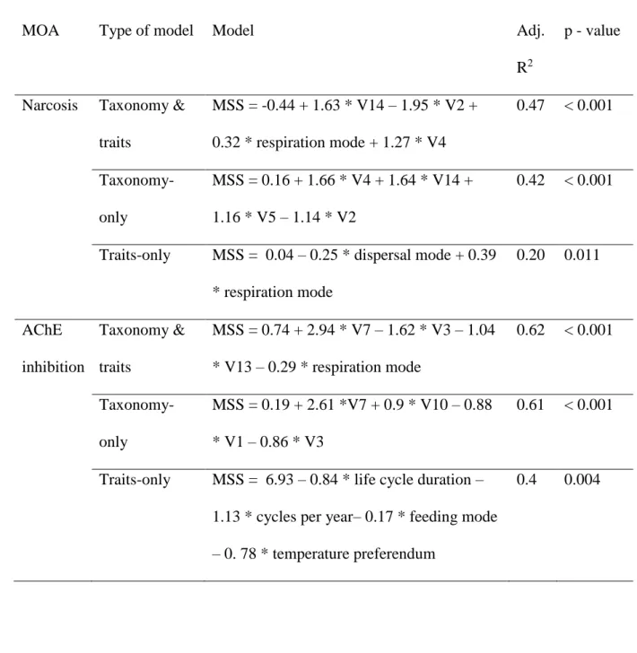
Table 1. Division of the 685 reference sites into the 7 super-groups, along with a description
256
of the dominant characteristics of the super-groups (taken from Davy-Bowker et al., 2008). 257 RIVPACS super-group N sites Dominant characteristics
1 64 All in Scotland, mostly islands
2 148 Upland streams, mainly in Scotland and Northern England
3 169 Intermediate rivers, South-East Scotland, Wales, North and South-West England 4 48 Small steeper streams, within 13 km of source
5 115 Intermediate size lowland streams, including chalk, South-East England 6 84 Small lowland streams, including chalk, South-East England
7 57 Larger, lowland streams, South-East England, larger, finer sediments 258
3. Results
259
3.1. Sensitivity models 260
Incorporating taxonomic relatedness slightly improved the predictive capacity of models for 261
invertebrate sensitivity towards narcotic and AChE inhibiting chemicals (higher adjusted R2), 262
compared to models without taxonomy (Table 2). Interestingly, the trait ‘mode of respiration’ 263
was incorporated in the taxonomy & traits model of narcosis (Figure A.3) and was also 264
present in the traits-only model. For AChE inhibition, mode of respiration was included in the 265
taxonomy & traits model (Figure A.4), but not in the traits-only model. Considering the 266
taxonomic predictors, V14, V2 and V4 were present in both the taxonomy-only and the 267
taxonomy & traits model for narcosis. For AChE inhibition, the predictors V7 and V3 were 268
present in both the taxonomy-only and the taxonomy & traits model. 269
13
Table 2. Predictive models constructed for narcotic and AChE inhibiting chemicals, in- and
271
excluding taxonomy. Taxonomic predictors are indicated with a V. See Figures A.3 and A.4 272
for a visualization of the predictors incorporated in the taxonomy & traits models. 273
MOA Type of model Model Adj.
R2
p - value
Narcosis Taxonomy & traits MSS = -0.44 + 1.63 * V14 – 1.95 * V2 + 0.32 * respiration mode + 1.27 * V4 0.47 < 0.001 Taxonomy-only MSS = 0.16 + 1.66 * V4 + 1.64 * V14 + 1.16 * V5 – 1.14 * V2 0.42 < 0.001
Traits-only MSS = 0.04 – 0.25 * dispersal mode + 0.39 * respiration mode 0.20 0.011 AChE inhibition Taxonomy & traits MSS = 0.74 + 2.94 * V7 – 1.62 * V3 – 1.04 * V13 – 0.29 * respiration mode 0.62 < 0.001 Taxonomy-only MSS = 0.19 + 2.61 *V7 + 0.9 * V10 – 0.88 * V1 – 0.86 * V3 0.61 < 0.001
Traits-only MSS = 6.93 – 0.84 * life cycle duration – 1.13 * cycles per year– 0.17 * feeding mode – 0. 78 * temperature preferendum
0.4 0.004
274
Cross-validation of the model species resulted in the correct classification of 82% and 74% of 275
the genera as sensitive or tolerant for respectively narcosis and AChE inhibiting chemicals 276
(Figure 1). For narcosis, the Diptera Paratanytarsus and Mochlonyx, the Odonata 277
Ophiogompus, the Ephemeroptera Siphlonurus, the Gastropoda Aplexa, and the Annelida
278
Chaetogaster were misclassified (predicted on the wrong side of the zero line). For AChE
14
inhibition, incorrect predictions were made in only two taxonomic groups, the Diptera 280
Glyptotendipes, Paratanytarsus, Tanytarsus, and the Odonata Anax, Crocothemis,
281
Ophiogompus and Orthetrum.
282
283
Figure 1. Observed MSS values (filled squares) and values predicted (unfilled circles) using
284
traits and taxonomy according to the best models for (a) narcotic (b) and AChE inhibiting 285
chemicals. 286
3.2. European freshwater ecoregions 287
3.2.1. Data availability. 288
For the ER communities, taxonomic data was available for 97% of the species, and covered 289
four crustacean orders (Amphipoda, Anostraca, Decopoda, and Isopoda), and six insect orders 290
(Coleoptera, Diptera, Ephemeroptera, Lepidoptera, Plecoptera and Trichoptera). Figure A.5 291
shows the taxonomic composition of all ERs at the order level. For 19% of these species there 292
was no or incomplete trait data available, leading to the exclusion of these species from our 293
analysis. Of the remaining species, only around 5% had toxicity data available. We therefore 294
15
had to predict the sensitivity of around 95% of the species for which no toxicity data was 295
available using the taxonomy & traits models for narcosis and AChE inhibition. 296
3.2.2. Taxonomic pattern. 297
On the continental scale, 46 and 33% of the species were found sensitive (MSS < 0) towards 298
narcotic and AChE inhibiting chemicals, respectively. For narcotic chemicals, 18 families 299
contained only genera predicted as sensitive. Among these 18 families were all families 300
belonging to the order of Isopoda (1 family), as well as a part of the Amphipoda (1 family), 301
Plecoptera (6), and Trichoptera (10) families included in our study (Table A.1). Five families 302
contained both sensitive and tolerant genera. Four of these families belonged to the order of 303
the Trichoptera, and one to the order of Lepidoptera. The remaining 25 families were 304
predicted to only contain tolerant genera (MSS > 0), and included all of the families 305
belonging to the order of Anostraca (1 family), Decapoda (5), Diptera (1), and Ephemeroptera 306
(12), as well as the remaining Amphipoda (2 families), Plecoptera (1), and Trichoptera (3) 307
families included in this study (Table A.2). 308
For AChE inhibiting chemicals, there was little variation in sensitivity of the genera 309
belonging to the same family, and the whole family was either predicted to contain only 310
sensitive (MSS < 0) or only tolerant (MSS > 0) genera. All genera belonging to the order of 311
the Trichoptera and all genera belonging to the family of the Gammaridae were predicted as 312
sensitive (Table A.3), while all other families included in this study were predicted to contain 313
only tolerant genera (Table A.4). 314
3.2.3. Geographical pattern. 315
For both MOAs, we noticed that the South of Europe (e.g. ER 1) has the highest proportion of 316
sensitive species (MSS < 0), whilst Iceland (ER 19) is the ecoregion containing the lowest 317
proportion of sensitive species (Figure 2). Central Europe (e.g. ER 14) contains the lowest 318
16
percentages of sensitive species. ER 6 contains the largest percentage (57%) of species 319
sensitive to narcotic chemicals, whilst ER 24 contains the largest percentage (45%) of species 320
sensitive to AChE inhibiting chemicals. 321
When comparing the assigned sensitivity class of each ER for the two MOAs, we find that 8 322
of the 25 ERs were grouped into the same class for both MOAs (ER 1, 3, 5, 11, 18, 19, 21, 24, 323
Figure A.5). ER 2, 4, and 6 -10 were classified one or two classes lower for sensitivity 324
towards AChE inhibiting chemicals compared to sensitivity towards narcotic chemicals, 325
whilst the opposite was true for ER 12 -17, 20, 22, 23, and 25 (Figure A.6). 326
17 327
Figure 2. Percentage of sensitive taxa (MSS < 0) to narcotic (a) and AChE inhibiting (b) chemicals in European freshwater ecoregions. The
328
numbers refer to the ecoregion number (ER 1 through ER 25). 329
18
3.3. RIVPACS river types 330
3.3.1. Data availability. 331
For the RIVPACS end-group communities, taxonomic data was available for 98% of the 332
species. To ensure that model predictions did not trespass the taxonomic range on which the 333
model was calibrated, any phylum that was not represented by one of the model species was 334
removed from the analysis. Consequently, sensitivity towards narcotic chemicals was 335
predicted for genera belonging to the phyla Annelida, Mollusca, and Arthropoda, whilst 336
sensitivity towards AChE inhibiting chemicals was predicted only for Arthropoda. 337
Coincidentally, in case of both datasets (Annelida, Mollusca, and Arthropoda, versus 338
Arthropoda only), 34% of the species had no or incomplete traits data available, leading to the 339
exclusions of these species from the analysis. Of the remaining species, less than 10% had 340
toxicity data available. We therefore had to predict the sensitivity of 90% of the species for 341
which no toxicity data was available using the taxonomy & traits models for narcosis and 342
AChE inhibition. 343
3.3.2. Taxonomic pattern. 344
Within the UK, 38, and 25% of the species were found sensitive (MSS < 0) to narcotic and 345
AChE inhibiting chemicals respectively. For narcotic chemicals, 37 families contained only 346
genera predicted as sensitive, with an MSS value below zero. Among these 37 families were 347
all families belonging to the order of Annelida (9 families), Isopoda (1), and Odonata (7), as 348
well as a part of the Amphipoda (1), Plecoptera (6), Trichoptera (8), and Gastropoda (5) 349
families included in our study (Table A.5). Four families contained both sensitive and tolerant 350
genera, all of them belonging to the order of Trichoptera. The 49 remaining families were 351
predicted to only contain tolerant genera, with an MSS value above zero. Among them were 352
all families belonging to the order of Arguloida (1 family), Coleoptera (7), Decapoda (1), 353
19
Diptera (5), Ephemeroptera (9), Hemiptera (7), Lepidoptera (1), Megaloptera (1), Neuroptera 354
(2), and Bivalvia (4), as well as the remaining Amphipoda (3), Plecoptera (1), Trichoptera (3), 355
and Gastropoda (4) families (Table A.6). 356
For AChE inhibiting chemicals, there was little variation in sensitivity of the genera 357
belonging to the same family, and, as for the ER assemblages, the whole family was either 358
predicted to only contain sensitive (MSS < 0) or tolerant (MSS > 0) genera. In total, 25 359
families contained genera that were all predicted as sensitive. This encompassed all families 360
belonging to the order of Trichoptera (15 families), as well as a part of the Amphipoda (1), 361
Diptera (2), Neuroptera (1), and Odonata (6) families (Table A.7). The remaining 43 362
Arthropod families were predicted to only contain tolerant species, and included all Arguloida 363
(1 family), Coleoptera (7), Decapoda (1), Ephemeroptera (9), Hemiptera (7), Isopoda (1), 364
Lepidoptera (1), Megaloptera (1), and Plectopera (7), as well as the rest of the Amphipoda (3), 365
Diptera (3), Neuroptera (1), and Odonata (1) families (Table A.8). 366
3.3.3. Geographical pattern. 367
Considering the RIVPACS sites, geographical patterns show opposite results for the two 368
MOAs (Figure 3). Regions containing more species sensitive towards narcotic chemicals were 369
observed in the west and north of the UK, while regions containing more species sensitive 370
towards AChE inhibiting chemicals were found in the south, south-west of the UK (Figure 3). 371
RIVPACS sites located in small to intermediate lowland streams contained more sensitive 372
species towards AChE inhibiting chemicals (super-groups 3, 4 and primarily 5, boxplots 373
Figure 3), whilst for narcotic chemicals most sensitive species were found at sites located in 374
upland rivers, mainly located in Scotland and Northern England (super-groups 1 and 2, 375
boxplots Figure 3). For both MOAs, larger, lowland streams located in South-East England 376
(super-group 7), contained the smallest percentage of sensitive species. 377
20 378
Figure 3. Map of the UK showing the percentage of sensitive taxa (MSS < 0) present at all
379
RIVPACS sites, and boxplots of the percentage of sensitive species (MSS < 0) present in each 380
RIVPACS super-group to narcotic and AChE inhibiting chemicals. Letters in boxplots 381
indicate significant differences (p < 0.05). 382
4. Discussion
383
4.1. Traits and taxonomic predictor selection, and how this can be improved 384
For both MOAs, mode of respiration was selected as an important trait for explaining species 385
sensitivity (Table 2). Several studies have investigated the relationship between respiration 386
and AChE inhibiting chemicals before (Buchwalter, Jenkins, & Curtis, 2002; Rico & Van den 387
Brink, 2015; Rubach et al., 2012; Rubach et al., 2010; van den Berg et al., 2019), and have 388
frequently found respiration important for determining species sensitivity, primarily due to an 389
21
influence of respiration mode on uptake rates. The relationship between narcosis and 390
respiration has been studied less, and there is to our knowledge only one study available that 391
performed an analysis with narcotic chemicals (van den Berg et al., 2019). The result of that 392
study closely aligns with ours, undoubtedly due to the large overlap in the data included in 393
both studies. 394
We find that combining traits with taxonomic information results in models with increased 395
predictive power, although only marginal (Table 2). Previous studies likewise emphasize the 396
importance of complementing traits approaches with taxonomic approaches (Pilière et al., 397
2016; Poff et al., 2006; Poteat et al., 2015). For example, Pilière and colleagues (2016) used 398
boosted regression tree modelling to assess the environmental responses of single traits, 399
orders and trait profile groups. They found that taxa belonging to the same trait profile group 400
but to different orders showed different environmental responses. Similarly, they found that 401
taxa belonging to the same order but to different trait profile groups showed different 402
environmental responses (Pilière et al., 2016). This indicates that unique information related 403
to the evolutionary history was captured by the order of a taxon, whilst another part was 404
captured by the trait set of a taxon. We find a similar result in our study, where the taxonomy-405
only model explaining sensitivity towards narcotic chemicals has an explanatory power of 406
0.42. This explanatory power increases to 0.46 when traits are included (Table 2). For AChE 407
inhibition we see a similar result, although there the increase is only from 0.61 to 0.62 (Table 408
2). Although the increase of predictive power is only slight, the increase in mechanistic 409
explanation is large, since the traits reveal mechanistic information regarding species 410
sensitivity, and the taxonomic predictors point out taxa which show a different response to the 411
chemical. The taxonomic predictors can thereby focus future research on finding the actual 412
mechanisms that are different between these taxa. For this reason, both traits and taxonomy 413
should be taken into consideration simultaneously for maximum benefit to risk assessment. 414
22
Although our models already show a good fit on the available data (Table 2), we anticipate 415
that technological advances both in molecular and computational technologies will lead to an 416
improvement of our models over time. Applying sophisticated molecular approaches can help 417
with resolving the taxonomy of currently still problematic organism groups, for instance, by 418
increasingly basing taxonomy on DNA markers, ideally replacing taxonomy completely by 419
phylogenetics in due time (Hebert, Cywinska, Ball, & Dewaard, 2003). Additionally, basing 420
phylogenetic trees on key target genes associated with Adverse Outcome Pathways (AOPs) 421
might substantially improve phylogenetic predictive models for application in ecotoxicology 422
(e.g. LaLone et al., 2013). Furthermore, our models could improve with increased computing 423
power. Due to memory limitations and the structure of currently existing model selection 424
algorithms, we had to restrict the number of predictors going into the model selection process. 425
However, since we maintain strict rules to avoid overfitting (e.g. the use of AICc as a model 426
selection criterion and the use of a multivariate approach for the taxonomic predictors), it 427
would be possible to add more predictors to the model without increasing the chance of 428
overfitting. 429
4.2. Sensitivity patterns at European scale 430
At the continental scale, we predict that around half of the species are sensitive (MSS < 0) 431
towards narcotic chemicals. This matches our expectations, since MSS is a relative value, and 432
there is not any taxonomic group known that is particularly sensitive towards narcotic 433
compounds (Escher & Hermens, 2002). For AChE inhibiting chemicals we predict around 434
one third of the arthropod species to be sensitive (MSS < 0). This is less than found in the 435
sensitivity ranking of Rico and Van den Brink (2015), where on average 70% of the 436
Arthropoda were found sensitive towards AChE inhibiting chemicals (organophosphates and 437
carbamates). However, this difference likely originates from the fact that Rico and Van den 438
Brink (2015) also included non-arthropod species. Since MSS is a relative value, and 439
23
arthropod species are the most sensitive group towards AChE inhibiting chemicals, including 440
non-arthropod species will result in relatively more sensitive arthropod species. 441
Considering both MOAs, our predictions show that river basins in central Europe contain 442
fewer sensitive species than those situated in the south (Figure 2). We reason that this results 443
from, on the one hand, chemical exposure patterns before and during the period that Illies 444
recorded the community composition of the ERs (Illies, 1978), and on the other hand, from 445
more ancient phylogeographical and ecological processes. Indeed, the pattern we find 446
coincides with the emission pattern of multiple persistent organic contaminants commonly 447
used in the 1960s, around the time when Illies was constructing his species database (Illies, 448
1978). Chemicals like DDT (Dichloro-diphenyl-trichloroethane, Stemmler & Lammel, 2009), 449
lindane (Prevedouros, MacLeod, Jones, & Sweetman, 2004), mercury (Pacyna, Pacyna, 450
Steenhuisen, & Wilson, 2003), and PCDFs (polychlorinated dibenzofurans, Pacyna, Breivik, 451
Münch, & Fudala, 2003) were more extensively used in central Europe, potentially reducing 452
the occurrence of more sensitive species in those regions. However, we think that chemical 453
exposure was not the main determinant for species composition, primarily because Moog and 454
colleagues demonstrated that different ERs could always be differentiated from each other 455
based on their community composition, even when heavily impacted by chemical stress 456
(Moog, Schmidt-Kloiber, Ofenböck, & Gerritsen, 2004). Therefore, we argue that the main 457
cause for the geographical pattern we see lies in the phylogeography of Europe, in which 458
extreme climatic events wipe out more sensitive species, and mountainous regions 459
consecutively serve as refugia and biodiversity hotspots (Rahbek, Borregaard, Antonelli, et 460
al., 2019; Rahbek, Borregaard, Colwell, et al., 2019). During the last ice age, glaciers covered 461
the majority of northern Europe, forcing most species towards refugia present in southern 462
Europe or to ice free parts of high mountain areas (e.g. Schmitt & Varga, 2012). Indeed, there 463
is a large overlap in biodiversity hotspots (Médail & Quézel, 1999; Mittermeier, Myers, 464
24
Thomsen, Da Fonseca, & Olivieri, 1998; Rahbek, Borregaard, Colwell, et al., 2019) or so-465
called regions of large endemism (Deharveng et al., 2000), with regions containing the 466
highest percentage of sensitive species (Figure 2). Then after the last ice age, species 467
recolonized northern Europe from these southern refugia, which is confirmed by the fact that 468
almost all species occurring in northern European are also present in central and/or southern 469
Europe (Hering et al., 2009). The relatively higher sensitivity of ER 22 and 15 (especially 470
towards AChE inhibiting chemicals, Figure 2) can be explained due to migration of more 471
sensitive species from Siberian refugia, e.g. located in the Ural mountains (Bernard, Heiser, 472
Hochkirch, & Schmitt, 2011; Schmitt & Varga, 2012). 473
4.3. Sensitivity patterns at UK scale 474
We see that certain biases in the underlying data are revealed in the sensitivity patterns we 475
find for the UK. For instance, at a national scale, fewer species were considered sensitive 476
compared to the continental scale, both towards narcotic and AChE inhibiting chemicals. We 477
think this is caused by the interaction of two things. First, our models are biased in predicting 478
entire families as sensitive or tolerant, in some cases resulting in entire phyla being predicted 479
as sensitive or tolerant. Second, the RIVPACS communities are taxonomically uneven at 480
genus level, the level we used to predict species sensitivity. Indeed, dipterans make up around 481
40% of all genera present which all are predicted to be tolerant towards the two MOAs. In this 482
case, the taxonomic unevenness at genus level specifically, has a large influence on the 483
percentage of species sensitive at the national scale. When we compare the ER and RIVPACS 484
results at the family level, results between the two datasets are more consistent. For instance, 485
for the ER dataset we predict that 33, 59, and 86% of respectively Amphipoda, Trichoptera, 486
and Plecoptera families were sensitive towards narcotic compounds. This was 25, 53, and 487
86% of the families in the same orders in the RIVPACS dataset. 488
25
The geographical distribution of sensitive species throughout the United Kingdom is less 489
pronounced than at a European level, although the opposing results of the RIPVAC super-490
groups towards the two MOAs studied is striking. This contradictory result corresponds with 491
the study of Van den Berg et al. (2019), where an inclusive database approach reveals large 492
differences in species sensitivity depending on MOA. Their study shows that AChE and 493
narcosis are on opposing ends of a dendrogram clustered on a matrix of species sensitivity 494
towards six diverse MOAs, indicating that AChE and narcosis show the largest differences in 495
species sensitivity among all MOAs tested. Additionally, we found alternative explanations 496
that could explain the contradicting geographical patterns we found for the two MOAs. 497
As an explanation for the geographical pattern for narcotic compounds, we find a large 498
overlap between hotspots of sensitivity towards narcotic toxicants and conservation areas in 499
the UK (e.g. with Special Areas of Conservation, Special Protection Areas, Sites of Special 500
Scientific Interest, (Gaston et al., 2006)). It is known that protected areas serve as 501
establishment centres, enabling the colonization of new regions by species that are shifting 502
their geographical ranges (Hiley, Bradbury, Holling, & Thomas, 2013; Thomas et al., 2012). 503
Although all RIVPACS sites are considered reference sites and have been selected because of 504
low anthropogenic influence, our results show that whether or not these sites are included or 505
in close proximity to a conservational area leads to a higher support of sensitive species, 506
likely due to an increased landscape and habitat heterogeneity. 507
As an explanation for the geographical pattern for AChE inhibiting compounds, the larger 508
differences between the sensitivity of super-groups towards AChE inhibiting chemicals 509
demonstrates that species sensitive towards AChE inhibition were more differentiated 510
according to river type (i.e. the abiotic preferences of the species) than according to the 511
availability of conservation areas. Additionally, the finding that the North to South pattern 512
that we found at a European level was not noticeably present at the UK level is probably due 513
26
to smaller differences in environmental factors (e.g. temperature, precipitation, 514
phylogeographic history) when considering the UK only, compared to when the whole of 515
Europe is considered. 516
4.4. Implications and outlook 517
Our analysis indicates that not only the taxonomic resolution of available trait databases is 518
crucial, also the resolution of the model is important. Additionally, we are confident that our 519
models will improve in the near future, for instance by the replacement of the taxonomic tree 520
with a phylogenetic tree based on validated biomarkers (for instance, as in Simões et al., 521
2019). In that case, the successful application of our suggested approach is mainly limited by 522
access to raw biological data (e.g. species abundance), which is currently still problematic 523
because governmental agencies provide ecological status information based on general 524
indices rather than species counts. Providing access to raw data, along with clear metrics on 525
the quality of that data (e.g. meeting the criteria defined in Moermond, Kase, Korkaric, & 526
Ågerstrand, 2016), would foster our understanding of the links between anthropogenic 527
stressors and populations or communities. Subsequently combining this effect data with 528
chemical concentration data would be the next logical step, and would require chemical 529
concentration data on all chemicals that are being monitored, not only priority substances, to 530
be made widely available by governmental agencies. 531
The current analysis provides an important new chapter in the development of environmental 532
scenarios that can be used for the environmental risk assessment of chemicals at larger 533
geographical scales (Franco et al., 2016; Rico et al., 2016). Our work is the first attempt to 534
apply sensitivity models on community assemblage data previously grouped according to both 535
biotic and abiotic parameters (e.g. invertebrate community composition, water depth, 536
alkalinity and temperature, Davy-Bowker et al., 2008). This combination of both biological 537
27
and spatial data is required to successfully characterize exposure, effects and recovery of 538
aquatic non-target species under realistic worst-case conditions. Currently, mismatches exist 539
between parameter values and spatial-temporal scales of ecological models used to predict 540
potential effects of chemicals (Rico et al., 2016). Our approach contributes to solving this 541
mismatch by simultaneously incorporating biological and environmental factors. 542
In addition to this, the inclusion of traits in our models leads to an increased mechanistic 543
understanding of cause-effect relationships, and allows for the application across wide 544
biogeographical regions. This extrapolation enables, for instance, the comparison of 545
ecological status across countries or regions that have so far remained unmonitored due to 546
practical reasons (e.g. remote regions), for instance, by using species assemblages predicted 547
by means of species distribution models (e.g. as in He et al., 2015). Also, patterns across wide 548
geographical scales can easily be compared with other studies by means of geographical 549
information systems (GIS) and simple additive models to reveal regions where multiple 550
stressors might be causing an effect simultaneously (e.g. as in Figure A.6, and see Vaj, 551
Barmaz, Sørensen, Spurgeon, & Vighi, 2011 for an example study). Take, for instance, the 552
potential impact of climate change on aquatic insects. Hering et al. (2009) show that southern 553
European regions contain the highest fraction of species sensitive towards climate change. 554
Since this largely overlaps with the regions we found to be most sensitive towards chemical 555
stressors (Figure 2), there might be an increased overall effect on aquatic communities due to 556
an unexpected interaction between climate change and chemical stress. In the north-east of 557
Europe, a similar amplification effect may occur due to an overlap in regions with a relatively 558
high chemical sensitivity (Figure 2), and predicted increased potential of harmful arthropod 559
pest invasions (Bacon, Aebi, Calanca, & Bacher, 2014). 560
Finally, our study demonstrates that sensitivity towards chemical stressors is spatially 561
variable, and that although entire regions can be considered relatively tolerant, there might 562
28
still be certain river reaches with a large percentage of sensitive species. Applied at relevant 563
geographic scales, the methodology described in this study has demonstrated the potential to 564
identify hotspots of sensitive species for given chemical classes. When applied to current risk 565
assessment approaches, this will both increase the biological realism of assessments, and 566
reduce the need for overly conservative assessment factors. 567
Acknowledgements
568
This work was supported by Unilever under the title ‘Ecological scenarios and models for use 569
in risk assessment’ (ESMU). There are no conflicts of interest. 570
Appendix A. Supplementary material
571
Supplementary data to this article can be found online at insert DOI. The R project, along 572
with all scripts and data necessary to reproduce the models and figures performed in this study 573
are available at Figshare (10.6084/m9.figshare.11294450) (van den Berg, 2019). 574
References
575
Bacon, S. J., Aebi, A., Calanca, P., & Bacher, S. (2014). Quarantine arthropod invasions in Europe: the role of
576
climate, hosts and propagule pressure. Diversity and distributions, 20(1), 84-94.
577
Baert, J. M., De Laender, F., & Janssen, C. R. (2017). The Consequences of Nonrandomness in
Species-578
Sensitivity in Relation to Functional Traits for Ecosystem-Level Effects of Chemicals. Environmental
579
Science & Technology, 51(12), 7228-7235. doi:10.1021/acs.est.7b00527 580
Barron, M. G., Lilavois, C. R., & Martin, T. M. (2015). MOAtox: A comprehensive mode of action and acute
581
aquatic toxicity database for predictive model development. Aquat Toxicol, 161, 102-107.
582
doi:10.1016/j.aquatox.2015.02.001
583
Benson, D. A., Karsch-Mizrachi, I., Lipman, D. J., Ostell, J., & Sayers, E. W. (2009). GenBank. Nucleic Acids
584
Res, 37(Database issue), D26-31. doi:10.1093/nar/gkn723 585
Bernard, R., Heiser, M., Hochkirch, A., & Schmitt, T. (2011). Genetic homogeneity of the Sedgling Nehalennia
586
speciosa (Odonata: Coenagrionidae) indicates a single Würm glacial refugium and trans-Palaearctic
587
postglacial expansion. Journal of Zoological Systematics and Evolutionary Research, 49(4), 292-297.
588
doi:10.1111/j.1439-0469.2011.00630.x
589
Buchwalter, D., Jenkins, J., & Curtis, L. (2002). Respiratory strategy is a major determinant of [3H] water and
590
[14C] chlorpyrifos uptake in aquatic insects. Canadian Journal of Fisheries and Aquatic Sciences,
591
59(8), 1315-1322. 592
Cairns, J. J. (1986). The Myth of the Most Sensitive SpeciesMultispecies testing can provide valuable evidence
593
for protecting the environment. BioScience, 36(10), 670-672. Retrieved from
594
http://dx.doi.org/10.2307/1310388
595
Chamberlain, S., & Szöcs, E. (2013). taxize - taxonomic search and retrieval in R.: F1000Research.
596
Chevenet, F., Dolédec, S., & Chessel, D. (1994). A fuzzy coding approach for the analysis of long‐term
597
ecological data. Freshwater Biology, 31(3), 295-309.
598
Davy-Bowker, J., Clarke, R. T., Corbin, T., Vincent, H., Pretty, J., Hawczak, A., . . . Jones, I. (2008). River
599
invertebrate classification tool.
600
De Laender, F., Morselli, M., Baveco, H., Van den Brink, P. J., & Di Guardo, A. (2015). Theoretically exploring
601
direct and indirect chemical effects across ecological and exposure scenarios using mechanistic fate
29
and effects modelling. Environment International, 74, 181-190.
603
doi:https://doi.org/10.1016/j.envint.2014.10.012
604
Deharveng, L., Dalens, H., Drugmand, H., Simon-Benito, J. C., Da Gama, M. M., Sousa, P., . . . Bedos, A.
605
(2000). Endemism mapping and biodiversity conservation in western Europe: an Arthropod
606
perspective. Belgian Journal of Entomology, 2, 59-75.
607
Escher, B. I., & Hermens, J. L. M. (2002). Modes of Action in Ecotoxicology: Their Role in Body Burdens,
608
Species Sensitivity, QSARs, and Mixture Effects. Environmental Science & Technology, 36(20),
4201-609
4217. doi:10.1021/es015848h
610
Franco, A., Price, O. R., Marshall, S., Jolliet, O., Van den Brink, P. J., Rico, A., . . . Ashauer, R. (2016). Towards
611
refined environmental scenarios for ecological risk assessment of down-the-drain chemicals in
612
freshwater environments. Integrated Environmental Assessment and Management, n/a-n/a.
613
doi:10.1002/ieam.1801
614
Gaston, K. J., Charman, K., Jackson, S. F., Armsworth, P. R., Bonn, A., Briers, R. A., . . . Kunin, W. E. (2006).
615
The ecological effectiveness of protected areas: the United Kingdom. Biological Conservation, 132(1),
616
76-87.
617
Griffith, D. A., & Peres-Neto, P. R. (2006). Spatial modeling in ecology: the flexibility of eigenfunction spatial
618
analyses. Ecology, 87(10), 2603-2613. doi:doi:10.1890/0012-9658(2006)87[2603:SMIETF]2.0.CO;2
619
Guénard, G. (2018). A phylogenetic modelling tutorial using Phylogenetic Eigenvector Maps (PEM) as
620
implemented in R package MPSEM (0.3-4). In.
621
Guénard, G., Legendre, P., & Peres‐Neto, P. (2013). Phylogenetic eigenvector maps: a framework to model and
622
predict species traits. Methods in Ecology and Evolution, 4(12), 1120-1131.
623
Guénard, G., von der Ohe, P. C., Walker, S. C., Lek, S., & Legendre, P. (2014). Using phylogenetic information
624
and chemical properties to predict species tolerances to pesticides. Proceedings of the Royal Society of
625
London B: Biological Sciences, 281(1789), 20133239. 626
He, K. S., Bradley, B. A., Cord, A. F., Rocchini, D., Tuanmu, M. N., Schmidtlein, S., . . . Pettorelli, N. (2015).
627
Will remote sensing shape the next generation of species distribution models? Remote Sensing in
628
Ecology and Conservation, 1(1), 4-18. 629
Hebert, P. D., Cywinska, A., Ball, S. L., & Dewaard, J. R. (2003). Biological identifications through DNA
630
barcodes. Proceedings of the Royal Society of London. Series B: Biological Sciences, 270(1512),
313-631
321.
632
Hering, D., Schmidt-Kloiber, A., Murphy, J., Lücke, S., Zamora-Munoz, C., López-Rodríguez, M. J., . . . Graf, W.
633
(2009). Potential impact of climate change on aquatic insects: a sensitivity analysis for European
634
caddisflies (Trichoptera) based on distribution patterns and ecological preferences. Aquatic Sciences,
635
71(1), 3-14. 636
Hiley, J. R., Bradbury, R. B., Holling, M., & Thomas, C. D. (2013). Protected areas act as establishment centres
637
for species colonizing the UK. Proceedings of the Royal Society B: Biological Sciences, 280(1760),
638
20122310.
639
Illies, J. (1978). Limnofauna europaea: Fischer Stuttgart.
640
Johnson, J. B., & Omland, K. S. (2004). Model selection in ecology and evolution. Trends Ecol Evol, 19(2),
101-641
108. doi:10.1016/j.tree.2003.10.013
642
LaLone, C. A., Villeneuve, D. L., Burgoon, L. D., Russom, C. L., Helgen, H. W., Berninger, J. P., . . . Ankley, G.
643
T. (2013). Molecular target sequence similarity as a basis for species extrapolation to assess the
644
ecological risk of chemicals with known modes of action. Aquatic toxicology, 144, 141-154.
645
Legendre, P., & Legendre, L. F. (2012). Numerical ecology (Vol. 24): Elsevier.
646
Lumley, T., & Miller, A. (2017). Leaps: Regression Subset Selection. Retrieved from
https://CRAN.R-647
project.org/package=leaps
648
Malaj, E., Guénard, G., Schäfer, R. B., & Van der Ohe, P. C. (2016). Evolutionary patterns and physicochemical
649
properties explain macroinvertebrate sensitivity to heavy metals. Ecological applications, 26(4),
1249-650
1259.
651
Maltby, L., Blake, N., Brock, T. C. M., & Van den Brink, P. J. (2005). Insecticide species sensitivity distributions:
652
Importance of test species selection and relevance to aquatic ecosystems. Environmental Toxicology
653
and Chemistry, 24(2), 379-388. doi:doi:10.1897/04-025R.1 654
Médail, F., & Quézel, P. (1999). Biodiversity Hotspots in the Mediterranean Basin: Setting Global Conservation
655
Priorities. Conservation biology, 13(6), 1510-1513. doi:10.1046/j.1523-1739.1999.98467.x
656
Mendiburu, F. d. (2017). agricolae: Statistical Procedures for Agricultural Research. [R package]. Retrieved
657
from https://CRAN.R-project.org/package=agricolae
658
Mittermeier, R. A., Myers, N., Thomsen, J. B., Da Fonseca, G. A., & Olivieri, S. (1998). Biodiversity hotspots
659
and major tropical wilderness areas: approaches to setting conservation priorities. Conservation
660
biology, 12(3), 516-520. 661
Moermond, C. T., Kase, R., Korkaric, M., & Ågerstrand, M. (2016). CRED: Criteria for reporting and evaluating
662
ecotoxicity data. Environmental Toxicology and Chemistry, 35(5), 1297-1309.
663
Moog, O., Schmidt-Kloiber, A., Ofenböck, T., & Gerritsen, J. (2004). Does the ecoregion approach support the
664
typological demands of the EU ‘Water Framework Directive’? In Integrated assessment of running
665
waters in Europe (pp. 21-33): Springer. 666
Nagai, T. (2016). Ecological effect assessment by species sensitivity distribution for 68 pesticides used in
667
Japanese paddy fields. Journal of Pesticide Science, 41(1), 6-14. doi:10.1584/jpestics.D15-056
668
Pacyna, J. M., Breivik, K., Münch, J., & Fudala, J. (2003). European atmospheric emissions of selected
669
persistent organic pollutants, 1970–1995. Atmospheric Environment, 37, 119-131.
670
Pacyna, J. M., Pacyna, E. G., Steenhuisen, F., & Wilson, S. (2003). Mapping 1995 global anthropogenic
671
emissions of mercury. Atmospheric Environment, 37, 109-117.
672
Pagel, M. (1999). Inferring the historical patterns of biological evolution. Nature, 401, 877. doi:10.1038/44766
673
Pebesma, E. J., & Bivand, R. S. (2005). Classes and methods for spatial data in R. R news, 5(2), 9-13.