RESEARCH OUTPUTS / RÉSULTATS DE RECHERCHE
Author(s) - Auteur(s) :
Publication date - Date de publication :
Permanent link - Permalien :
Rights / License - Licence de droit d’auteur :
Bibliothèque Universitaire Moretus Plantin
Dépôt Institutionnel - Portail de la Recherche
researchportal.unamur.be
University of Namur
Solving the trust-region subproblem using the Lanczos method
Gould, Nick; Lucidi, Stefano; Roma, Massimo; Toint, Philippe
Published in:
SIAM Journal on Optimization
Publication date:
1999
Document Version
Early version, also known as pre-print
Link to publication
Citation for pulished version (HARVARD):
Gould, N, Lucidi, S, Roma, M & Toint, P 1999, 'Solving the trust-region subproblem using the Lanczos method',
SIAM Journal on Optimization, vol. 9, no. 2, pp. 504-525.
General rights
Copyright and moral rights for the publications made accessible in the public portal are retained by the authors and/or other copyright owners and it is a condition of accessing publications that users recognise and abide by the legal requirements associated with these rights. • Users may download and print one copy of any publication from the public portal for the purpose of private study or research. • You may not further distribute the material or use it for any profit-making activity or commercial gain
• You may freely distribute the URL identifying the publication in the public portal ?
Take down policy
If you believe that this document breaches copyright please contact us providing details, and we will remove access to the work immediately and investigate your claim.
N. I. M. Gould1, S. Lucidi2,
M. Roma2 and Ph. L. Toint3
Report 97/11 11 June 1997
1 Rutherford Appleton Laboratory,
Chilton, Oxfordshire OX11 0QX, England Email: [email protected]
Current reports available by anonymous ftp from the directory “pub/reports” on joyous-gard.cc.rl.ac.uk
2
Department of Mathematics University “La Sapienza”
Rome, Italy
Email:[email protected] and [email protected]
3
Department of Mathematics, Facult´es Universitaires ND de la Paix 61, rue de Bruxelles, B-5000 Namur, Belgium
Email: [email protected]
Current reports available by anonymous ftp from the directory “pub/reports” on thales.math.fundp.ac.be
N. I. M. Gould, S. Lucidi, M. Roma and Ph. L. Toint 11 June 1997
Abstract
The approximate minimization of a quadratic function within an ellipsoidal trust region is an important subproblem for many nonlinear programming methods. When the number of variables is large, the most widely-used strategy is to trace the path of conjugate gradient iterates either to convergence or until it reaches the trust-region boundary. In this paper, we investigate ways of continuing the process once the boundary has been encountered. The key is to observe that the trust-region problem within the currently generated Krylov subspace has very special structure which enables it to be solved very efficiently. We compare the new strategy with existing methods. The resulting software package is available as HSL VF05 within the Harwell Subroutine Library.
1
Introduction
Trust-region methods for unconstrained minimization are blessed with both strong theoretical convergence properties and a good reputation in practice. The main computational step in these methods is to find an approximate minimizer of some model of the true objective function within a “trust” region for which a suitable norm of the correction lies within a given bound. This restriction is known as the trust-region constraint, and the bound on the norm is its radius. The radius is adjusted so that successive model problems mimic the true objective within the trust region.
The most widely-used models are quadratic approximations to the objective function, as these are simple to manipulate and may lead to rapid convergence of the underlying method. From a theoretical point of view, the norm which defines the trust region is irrelevant so long as it is “uniformly” related to the ℓ2norm. From a practical perspective, this choice certainly affects the
subproblem, and thus the methods one can consider when solving it. The most popular practical choices are the ℓ2- and ℓ∞-norms, and weighted variants thereof. In our opinion, it is important
that the choice of norm reflects the underlying geometry of the problem; simply picking the ℓ2-norm may not be adequate when the problem is large, and the eigenvalues of the Hessian of
the model widely spread. We believe that weighting the norm is essential for many large-scale problems.
In this paper, we consider the solution of the quadratic-model trust-region subproblem in a weighted ℓ2-norm. We are interested in solving large problems, and thus cannot rely solely on
factorizations of the matrices involved. We thus concentrate on iterative methods. If the model of the Hessian is known to be positive definite and the trust-region radius sufficiently large that the trust-region constraint is inactive at the unconstrained minimizer of the model, the obvious way to solve the problem is to use the preconditioned conjugate-gradient method. Note that the role of the preconditioner here is the same as the role of the norm used for the trust-region, namely to change the underlying geometry so that the Hessian in the rescaled space is better conditioned. Thus, it will come as no surprise that the two should be intimately connected. Formally, we shall require that the weighting in the ℓ2-norm and the preconditioning are performed by the same
matrix.
When the radius is smaller than a critical value, the unconstrained minimizer of the model will no longer lie within the trust-region, and thus the required solution will lie on the trust-region boundary. The simplest strategy in this case is to consider the piecewise linear path connecting the conjugate-gradient iterates, and to stop at the point where this path leaves the trust region. Such a strategy was first proposed independently by Steihaug (1983) and Toint (1981), and we shall refer to the terminating point as the Steihaug-Toint point. Remarkably, it is easy to establish the global convergence of a trust-region method based on such a simple strategy. The key is that global convergence may be proved provided that the accepted estimate of the solution has a model value no larger than at the Cauchy point (see Powell, 1975). The Cauchy point is simply the minimizer of the model within the trust-region along the preconditioned steepest-descent direction. As the first segment on the piecewise-linear conjugate-gradient path gives precisely this point, and as the model value is monotonically decreasing along the entire path, the Steihaug-Toint strategy ensures convergence.
If the model Hessian is indefinite, the solution must also lie on the trust-region boundary. This case may also be simply handled using preconditioned conjugate gradients. Once again the piecewise linear path is followed until either it leaves the trust-region, or a segment with negative curvature is found (a vector p is a direction of negative curvature if the inner product hp, Hpi < 0, where H is the model Hessian). In the latter case, the path is continued downhill along this direction of negative curvature as far as the constraint boundary. This variant was proposed by Steihaug (1983), while Toint (1981) suggests simply returning to the Cauchy point. As before, global convergence is ensured as either of these terminating points, as the objective function values there are no larger than at the Cauchy point. For consistency with the previous paragraph, we shall continue to refer to the terminating point in Steihaug’s algorithm as the Steihaug-Toint point, although strictly Toint’s point in this case may be different.
The Steihaug-Toint method is basically unconcerned with the trust region until it blunders into its boundary and stops. This is rather unfortunate, particularly as considerable experience has shown that this frequently happens during the first few, and often the first, iteration(s) when negative curvature is present. The resulting step is then barely, if at all, better than the Cauchy direction, and this may lead to a slow but globally convergent algorithm in theory and a barely convergent method in practice. In this paper, we consider an alternative which aims to avoid this drawback by trying harder to solve the subproblem when the boundary is encountered, while maintaining the efficiencies of the conjugate gradient method so long as the iterates lie interior.
The mechanism we use is the Lanczos method.
The paper is organized as follows. In Section 2 we formally define the problem and any notation that we will use. The basis of our new method is given in Section 3, while in Section 4, we will review basic properties of the preconditioned conjugate-gradient and Lanczos methods. Our new method is given in detail in Section 5. Some numerical experiments demonstrating the effectiveness of the approach are given in Section 6, and a number of conclusions and perspectives are drawn in the final section.
2
The trust-region subproblem and its solution
Let M be a symmetric positive-definite easily-invertible approximation to the symmetric matrix H. Furthermore, define the M -norm of a vector as
ksk2M = hs, Msi,
where h·, ·i is the usual Euclidean inner product. In this paper, we consider the M-norm trust-region problem
minimize
s∈Rn
q(s) ≡ hg, si +1
2hs, Hsi subject to kskM ≤ ∆, (2.1)
for some vector g and radius ∆ > 0.
A global solution to the problem is characterized by the following result.
Theorem 2.1 (Gay, 1981, Sorensen, 1982) Any global minimizer sM
of q(s) subject to kskM ≤ ∆ satisfies the equation
H(λM )sM = −g, (2.2) where H(λM ) ≡ H +λM is positive semi-definite, λM ≥ 0 and λM (ksM kM−∆) = 0. If H(λM) is positive definite, sM is unique.
This result is the basis of a series of related methods for solving the problem which are appropriate when forming factorizations of H(λ) ≡ H + λM for a number of different values of λ is realistic. For then, either the solution lies interior, and hence λM
= 0 and sM
= −H+g, or the solution lies
on the boundary and λM
satisfies the nonlinear equation
kH(λ)+gkM = ∆, (2.3)
where H+ denotes the pseudo-inverse of H. Equation (2.3) is straightforward to solve using a
safeguarded Newton iteration, except in the so-called hard case for which g lies in the null-space of H(λM). In this case, an additional vector in the range-space of H(λM) may be required if a solution
on the trust-region boundary is sought. Goldfeldt, Quandt and Trotter (1966), Hebden (1973) and Gay (1981) all proposed algorithms of this form. The most sophisticated algorithm to date, by Mor´e and Sorensen (1983), is available as subroutine GQTPAR in the MINPACK-2 package, and guarantees that a nearly optimal solution will be obtained after a finite number of factorizations. While such algorithms are appropriate for large problems with special Hessian structure — such as for band matrices — the demands of a factorization at each iteration limits their ap-plicability for general large problems. It is for this reason that methods which do not require factorizations are of interest.
Throughout the paper, we shall denote the k by k identity matrix by Ik, and its j-th column
and the matrix Qk= (q0· · · qk) formed from these vectors is an M -orthonormal matrix. The set
of vectors {pi} are H-conjugate (or H-orthogonal) if hpi, Hpji = 0 for i 6= j.
3
A new algorithm for large-scale trust-region subproblems
To set the scene for this paper, we recall that the Cauchy point may be defined as the solution to the problem
minimize
s ∈span{M−1g}
q(s) ≡ hg, si +1
2hs, Hsi subject to kskM ≤ ∆, (3.1)
that is as the minimizer of q within the trust region where s is restricted to the 1-dimensional subspace span©
M−1gª
. The dogleg methods (see, Powell, 1970, Dennis and Mei, 1979) aim to solve the same problem over a particular two-dimensional subspace (a one-dimensional arc), while Byrd, Schnabel and Schultz (1985) do the same over a general two-dimensional subspace. In each of these cases the solution is easy to find as the search space is small. The difficulty with the general problem (2.1) is that the search space Rn is large. This leads immediately to the
possibility of solving a compromise problem minimize
s ∈ S
q(s) subject to kskM ≤ ∆, (3.2)
where S is a specially chosen subspace of Rn.
Now consider the Steihaug-Toint algorithm at an iteration k before the trust-region boundary is encountered. In this case, the point sk+1 is the solution to (3.2) with the set
S = Kk def
= spannM−1g, (M−1H)M−1g, (M−1H)2M−1g, · · · , (M−1H)kM−1go, (3.3) the Krylov space generated by the starting vector M−1g and matrix M−1H. That is, the
Steihaug-Toint algorithm gradually widens the search space using the very efficient precondi-tioned conjugate gradient method. However, as soon as the Steihaug-Toint algorithm moves across the trust-region boundary, the terminating point sk+1 no longer necessarily solves the
problem (3.2) over the set (3.3), indeed it is very unlikely to do so when k > 0. (As the iterates generated by the method increase in M -norm, once an iterate leaves the trust region, the solution to (3.2)–(3.3), and thus (2.1), must lie on the boundary. See, Steihaug, 1983, Theorem 2.1, for details). Can we do better? Yes, by recalling that the preconditioned conjugate gradient and Lanczos methods generate different bases for the same Krylov space.
4
The preconditioned conjugate-gradient and Lanczos methods
The preconditioned conjugate-gradient and Lanczos methods may be viewed as efficient tech-niques for constructing different bases for the same Krylov space, Kk. The conjugate gradient
method aims for an H-conjugate basis, while the Lanczos method obtains an M -orthonormal basis.
Algorithm 4.1: The preconditioned conjugate gradient method
Set g0= g, and let v0 = M−1g0 and p0= −v0. For j = 0, 1, · · · , k − 1, perform the iteration,
αj = hgj, vji/hpj, Hpji (4.1)
gj+1 = gj+ αjHpj (4.2)
vj+1 = M−1gj+1 (4.3)
βj = hgj+1, vj+1i/hgj, vji (4.4)
pj+1 = −vj+1+ βjpj (4.5)
Algorithm 4.2: Preconditioned Lanczos method
Set t0 = g, w−1 = 0 and, for j = 0, 1, · · · , k, perform the iteration,
yj = M−1tj (4.6) γj = q htj, yji (4.7) wj = tj/γj (4.8) qj = yj/γj (4.9) δj = hqj, Hqji (4.10) tj+1 = Hqj− δjwj− γjwj−1 (4.11)
The conjugate gradient method generates the basis
Kk = span {p0, p1, · · · , pk} (4.12)
from Algorithm 4.1, while the Lanczos method generates the basis
with Algorithm 4.2. The Lanczos iteration is often written in the more compact form
HQk− MQkTk = γk+1wk+1eTk+1 and (4.14)
QTkM Qk = Ik+1 (4.15)
where Qk is the matrix (q0· · · qk), and the matrix
Tk= δ0 γ1 γ1 δ1 · · · · · δk−1 γk γk δk (4.16)
is tridiagonal. It then follows directly that
QTkHQk = Tk, (4.17)
QTkg = γ0e1 and (4.18)
g = M y0= γ0M q0. (4.19)
The two methods are intimately related. In particular, so long as the conjugate-gradient iteration does not break down, the Lanczos vectors may be recovered from the conjugate-gradient iterates as
qk= vk/
q
hgk, vki.
while the Lanczos tridiagonal may be expressed as
Tk= 1 α0 − √ β0 α0 − √ β0 α0 1 α1 + β0 α0 − √ β1 α1 − √ β1 α1 1 α2 + β1 α1 · · · · · αk1 −1 + βk −2 αk −2 − √ βk −1 αk −1 − √ βk −1 αk −1 1 αk + βk −1 αk −1 . (4.20)
The conjugate gradient iteration may breakdown if hpj, Hpji = 0, which can only occur if H is
not positive definite, and will stop if hgj, vji = 0. On the other hand, the Lanczos iteration can
only fail if Kj is an invariant subspace for M−1H.
If q(s) is convex in the manifold Kj+1, the minimizer sj+1 of q in this manifold satisfies
sj+1 = sj+ αjpj (4.21)
so long as the initial value s0 = 0 is chosen. Thus this estimate is easy to recur from the
conjugate-gradient iteration. The minimizers in successive manifolds may also be easily obtained using the Lanczos process, although the conjugate-gradient iteration is slightly less expensive, and thus to be preferred.
The vector gj+1 in the conjugate gradient method gives the gradient of q(s) at sj+1. It is
quite common to stop the method as soon as this gradient is sufficiently small, and the method naturally records the M−1-norm of the gradient, kgk+1kM−1 = hgj, vji. This norm is also available
in the Lanczos method as
gk+1= γk+1hek+1, hkiwk+1 and kgk+1kM−1 = γk+1|hek+1, hki|, (4.22)
where hk solves the tridiagonal linear system Tkhk+ γ0e1 = 0. The last component, hek+1, hki,
of hk is available as a further by-product.
5
The truncated Lanczos approach
Rather than use the preconditioned conjugate gradient basis {p0, p1, · · · , pk} for S, we shall use
the equivalent Lanczos M -orthonormal basis {q0, q1, · · · , qk}. The Lanczos basis has previously
been used by Nash (1984) — to convexify the quadratic model — and Lucidi and Roma (1997) — to compute good directions of negative curvature — within linesearch based methods for unconstrained minimization. We shall consider vectors of the form
s ∈ S = {s ∈ Rn| s = Qkh},
and seek
sk= Qkhk, (5.1)
where sk solves the problem
minimize
s ∈S
q(s) ≡ hg, si +1
2hs, Hsi subject to kskM ≤ ∆. (5.2)
It then follows directly from (4.15), (4.17) and (4.18) that hk solves the problem
minimize
h ∈ Rk+1
hh, γ0e1i + 12hh, Tkhi subject to khk2≤ ∆. (5.3)
There are a number of crucial observations to be made here. Firstly, it is important to note that the resulting trust-region problem involves the two-norm rather than the M -norm. Secondly, as Tk is tridiagonal, it is feasible to use the Mor´e-Sorensen algorithm to compute the model
minimizer even when n is large. Thirdly, having found hk, the matrix Qk is needed to recover
sk, and thus the Lanczos vectors will either need to be saved on backing store or regenerated.
As we shall see, we only need Qk once we are satisfied that continuing the Lanczos process will
give little extra benefit. Fourthly, one would hope that as a sequence of such problems may be solved, and as Tk only changes by the addition of an extra diagonal and superdiagonal entry,
solution data from one subproblem may be useful for starting the next. We consider this issue in Section 5.2.
The basic trust-region solution classification theorem, Theorem 2.1, shows that
where Tk+ λkIk+1 is positive semi-definite, λk ≥ 0 and λk(khkk2− ∆) = 0. What does this tell
us about sk? Firstly, using (4.17), (4.18) and (5.4) we have
QTk(H + λkM )sk= QTk(H + λkM )Qkhk= (Tk+ λkIk+1)hk= −γ0e1= −QTkg,
and additionally that
λk(kskkM − ∆) = 0 and λk≥ 0. (5.5)
Comparing these with the trust-region classification theorem, we see that sk is the Galerkin
approximation to sM
from the space spanned by Qk.
We may then ask how good the approximation is. In particular, what is the error (H + λkM )sk + g? The simplest way of measuring this error would be to calculate hk and λk by
solving (5.3), then to recover skas Qkhk and finally to substitute skand λk into (H + λM )s + g.
However this is inconvenient as it requires that we have easy access to Qk. Fortunately there is
a far better way.
Theorem 5.1
(H + λkM )sk+ g = γk+1hek+1, hkiwk+1 (5.6)
and
k(H + λkM )sk+ gkM−1 = γk+1|hek+1, hki|. (5.7)
Proof. We have that
Hsk = HQkhk = M QkTkhk+ γk+1hek+1, hkiwk+1 from (4.14) = −MQk(λkhk+ γ0e1) + γk+1hek+1, hkiwk+1 from (5.4) = −λkM Qkhk− γ0M Qke1+ γk+1hek+1, hkiwk+1 = −λkM sk− γ0M q0+ γk+1hek+1, hkiwk+1 = −λkM sk− g + γk+1hek+1, hkiwk+1 from (4.19) .
This then directly gives (5.6), and (5.7) follows from the M−1-orthonormality of w
k+1. ✷
Therefore we can indirectly measure the error (in the M−1-norm) knowing simply γ
k+1 and the
last component of hk, and we do not need skor Qkat all. Observant readers will notice the strong
similarity between this error estimate and the estimate (4.22) for the gradient of the model in the Lanczos method, but this is not at all surprising as the two methods are aiming for the same point if the trust-region radius is large enough. An interpretation of (5.7) is also identical to that of (4.22). The error will be small when either of γk+1 or the last component of hk is small.
We now consider the problem (5.3) in more detail. We say that a symmetric tridiagonal matrix is reducible if one or more of its off-diagonal entries is zero; otherwise it is irreducible. We then have the following preliminary result.
Lemma 5.2 (See also, Parlett, 1980, Theorem 7.9.5) Suppose that the tridiagonal matrix T is irreducible, and that v is an eigenvector of T . Then the first component of v is nonzero.
Proof. By definition
T v = θv, (5.8)
for some eigenvalue θ. Suppose that the first component of v is zero. Considering the first component of (5.8), we have that the second component of v is zero as T is tridiagonal and irreducible. Repeating this argument for the i-th component of (5.8), we deduce that the the i + 1-st component of v is zero for all i, and hence that v = 0. But this contradicts the assumption that v is an eigenvector, and so the first component of v cannot be zero. ✷ This immediately yields the following useful result.
Theorem 5.3 Suppose that Tk is irreducible. Then the hard case cannot occur for the
subproblem (5.3).
Proof. Suppose the hard case occurs. Then, by definition, γ0e1 is orthogonal to vk, the
eigenvector corresponding to the leftmost eigenvalue, −θk, of Tk. Thus, the first component of
vk is zero, which, following Lemma 5.2, contradicts the assumption that vk is an eigenvector.
Thus the hard case cannot occur. ✷
This result is important as it suggests that the full power of the Mor´e and Sorensen (1983) algorithm is not needed to solve (5.3). We shall return to this in Section 5.2. We also have an immediate corollary.
Corollary 5.4 Suppose that Tn−1 is irreducible. Then the hard case cannot occur for the
original problem (2.1).
Proof. When k = n − 1, the columns of Qn−1form a basis for Rn, Thus the problems (2.1)
and (5.2) are identical, and (5.2) and (5.3) are related through a nonsingular transformation. The result then follows directly from Theorem 5.3 in the case k = n − 1. ✷ Thus, if the hard case occurs for (2.1), the Lanczos tridiagonal must become reducible at some stage.
Theorem 5.5 Suppose that Tk is irreducible, that hk and λk satisfy (5.4) and that Tk+
λkIk+1 is positive semi-definite. Then Tk+ λkIk+1 is positive definite.
Proof. Suppose that Tk+ λkIk+1 is singular. Then there is a nonzero eigenvector vk for
which (Tk+ λkIk+1)vk = 0. Hence, combining this with (5.4) reveals that
0 = hhk, (Tk+ λkIk+1)vki = hvk, (Tk+ λkIk+1)hki = −γ0hvk, e1i,
and hence that the first component of vk is zero. But this contradicts Lemma 5.2. Hence
Tk+ λkIk+1 is both positive semi-definite and nonsingular, and thus positive definite. ✷
This result implies that (5.4) has a unique solution. We now consider this solution.
Theorem 5.6 Suppose that hek+1, hki = 0. Then Tk is reducible.
Proof. Suppose that Tk is irreducible. As the k + 1-st component of hk is zero, then from
the irreducibility of Tk and the k + 1-st equation of (5.4), we deduce that the k-th component
of hk is zero. Repeating this argument for the i + 1-st equation of (5.4), we deduce that the
i-th component of hk is zero for 1 ≤ i ≤ k, and hence that hk = 0. But this contradicts the
first equation of (5.4), and thus Tk must be reducible. ✷
Thus we see that of the two possibilities suggested by Theorem 5.1 for obtaining an sk for which
(H + λkM )sk+ g = 0, it will be the possibility γk+1= 0 that occurs before hek+1, hki = 0.
Theorem 5.7 Suppose that the hard case does not occur for (2.1), and that γk+1 = 0.
Then sk solves (2.1).
Proof. If γk+1 = 0, the Krylov space Kk is an invariant subspace of M−1H, and by
construction the first basis element of this space is M−1g. As the hard case does not occur
for (2.1), this space must also contain at least one eigenvector corresponding to the leftmost eigenvalue, −θ, of M−1H. Thus one of the eigenvalues of T
k must be −θ, and λk ≥ θ as
Tk+ λkIk+1 is positive semi-definite. But this implies that H + λkM is positive semi-definite,
which combines with (5.1), (5.5) and Theorem 5.1 with γk+1 = 0 to show that sk satisfies the
optimality conditions shown in Theorem 2.1. ✷
Thus we see that in the easy case, the required solution will be obtained from the first irreducible block of the Lanczos tridiagonal. It remains for us to consider the hard case. In view of
Corol-lary 5.4, this case can only occur when Tkis reducible. Suppose therefore that Tk reducibles into
ℓ blocks of the form
Tk= Tk1 Tk2 · Tkℓ , (5.9)
where each of the Tki defines an invariant subspace for M
−1H and where the last block T kℓ is
the first to yield the leftmost eigenvalue, −θ, of M−1H. Then there are two cases to consider.
Theorem 5.8 Suppose that the hard case occurs for (2.1), that Tk is as described by (5.9),
and the last block Tkℓ is the first to yield the leftmost eigenvalue, −θ, of M
−1H. Then,
1. if θ ≤ λk1, a solution to (2.1) is given by sk = Qk1hk1, where hk1 solves the
positive-definite system
(Tk1 + λk1Ik1+1)hk1 = −γ0e1.
2. if θ > λk1, a solution to (2.1) is given by sk= Qkhk, where
hk = h 0 · 0 αu , (5.10)
h is the solution of the nonsingular tridiagonal system (Tk1 + θIk1+1)h = −γ0e1,
u is an eigenvector of Tkℓ corresponding to −θ, and α is chosen so that
khk1k 2 2+ α 2 ku||22 = ∆ 2 .
Proof. In case 1, H +λk1M is positive semi-definite as λk1 ≥ θ, and the remaining optimality
conditions are satisfied as γk1+1 = 0 and hk1 solves (5.2). That Tk1 + λk1Ik1+1 is positive
definite follows from Theorem 5.5. In case 2, H +θM is positive semi-definite. Furthermore, as θ > λk1, it is easy to show that khk2 < khk1k2 ≤ ∆, and hence that there is a root α for which
kskkM = khkk2 = ∆. Finally, as each Qki defines an invariant subspace, HQki = M QkiTki.
Writing s = Qk1h and v = Qkℓu, we therefore have
Hs = HQk1h = M Qk1Tk1h = M Qk1(−θh − γ0e1) = −θMs − g
and
Thus (H + θM )sk= −g, and sk satisfies all of the optimality conditions for (5.2). ✷
Notice that to obtain sk as described in this theorem, we only require the Lanczos vectors
corre-sponding to blocks one and, perhaps, ℓ of Tk.
We do not claim that to solve the problem as outlined in Theorem 5.8 is realistic, as it relies on our being sure that we have located the left-most eigenvalue of M−1H. With Lanczos-type
methods, one cannot normally guarantee that all eigenvalues, including the leftmost, will be found unless one ensures that all invariant subspaces have been investigated, and this may prove to be very expensive for large problems. In particular, the Lanczos algorithm, Algorithm 4.2, terminates each time an invariant subspace has been determined, and must be restarted using a vector q which is M -orthonormal to the previous Lanczos directions. Such a vector may be obtained from the Gram-Schmidt process by re-orthonormalizing a suitable vector — a vector with some component M -orthogonal to the existing invariant subspaces, perhaps a random vector — with respect to the previous Lanczos directions, which means that these directions will have to be regenerated or reread from backing store. Thus, while this form of the solution is of theoretical interest, it is unlikely to be of practical interest if a cheap approximation to the solution is all that is required.
5.1 The algorithm
We may now outline our algorithm, Algorithm 5.1, the generalized Lanczos trust-region (GLTR) method. We stress that, as our goal is merely to improve upon the value delivered by the Steihaug-Toint method, we do not use the full power of Theorem 5.8, and are content just to investigate the first invariant subspace produced by the Lanczos algorithm. In almost all cases, this subspace contains the global solution to the problem, and the complications and costs required to implement a method based on Theorem 5.8 are, we believe, prohibitive in our context.
Algorithm 5.1: The generalized Lanczos trust-region method
Let s0 = 0, g0 = g, v0 = M−1g0, γ0 =
p
hv0, g0i and p0 = −v0. Set the flag INTERIOR as
true. For k = 0, 1, · · · until convergence, perform the iteration, αk = hgk, vki/hpk, Hpki
Obtain Tk from Tk−1 using (4.20)
If INTERIOR is true, but αk≤ 0 or ksk+ αkpkkM ≥ ∆, reset INTERIOR to false.
If INTERIOR is true sk+1 = sk+ αkpk
else
solve the tridiagonal trust-region subproblem (5.3) to obtain hk
end if
gk+1 = gk+ αkHpk
vk+1 = M−1gk+1
If INTERIOR is true
test for convergence using the residual kgk+1kM−1
else
test for convergence using the value γk+1|hek+1, hki|
end if
βk = hgk+1, vk+1i/hgk, vki
pk+1 = −vk+1+ βkpk
If INTERIOR is false, recover sk = Qkhk by rerunning the recurrences or obtaining Qk from
backing store.
When recovering sk= Qkhk by rerunning the recurrences, economies can be made by saving the
αi and βi during the first pass, and reusing them during the second. A potentially bigger saving
may be made if one is prepared to accept a slightly inferior value of the objective function. The idea is simply to save the value of q at each iteration. On convergence, one looks back through this list to find an iteration, ℓ say, for which a required percentage of the best value was obtained, recompute hℓ and then accept sℓ= Qℓhℓ as the required estimate of the solution. If the required
percentage occurs at an iteration before the boundary is encountered, both the final point before the boundary and the Steihaug-Toint point are suitable and available without the need for the second pass.
We note that we have used the conjugate-gradient method (Algorithm 4.1) to generate the Lanczos vectors. If the inner-product hpk, Hpki proves to be tiny, it is easy to continue using the
Lanczos method (Algorithm 4.2) itself; the vectors qj = vj/
q
hgj, vji and wj = gj/
q
required to continue the Lanczos recurrence (4.11) are directly calculable from conjugate-gradient method.
At each stage of both the Steihaug-Toint algorithm and our GLTR method (Algorithm 5.1), we need to calculate ksk+ αpkkM. This issue is not discussed by Steihaug as it is implicitly
assumed that M is available. However, it may be the case that all that is actually available is a procedure which returns M−1v for a given input v, and thus M is unavailable. Fortunately this
is not a significant drawback as it is possible to calculate ksk+ αpkkM from available information.
To see this, observe that
ksk+ αpkk2M = kskk2M+ 2αhsk, M pki + α2kpkk2M, (5.11)
and thus that we can find ksk+1k2M from kskk2M so long as we already know hsk, M pki and
kpkk2M. But it is straightforward to show that these quantities may be calculated from the pair
of recurrences hsk, M pki = βk−1 ³ hsk−1, M pk−1i + αk−1kpk−1k2M ´ and (5.12) kpkk2M = hgk, vki + β2k−1kpk−1k2M (5.13)
where, of course, hgk, vki has already been calculated as part of the preconditioned
conjugate-gradient method.
5.2 Solving the irreducible tridiagonal trust-region subproblem
In view of Theorem 5.3, the irreducible tridiagonal trust-region subproblem (5.3) is, in theory, easier to solve than the general problem. This is so both because the Hessian is tridiagonal (and thus very inexpensive to factorize), and because the hard case cannot occur. We should be cautious here, because the so-called “almost” hard case — which occurs when g only has a tiny component in the range-space of H(λM
) — may still happen, and the trust-region problem in this case is naturally ill conditioned and thus likely to be difficult to solve.
The Mor´e and Sorensen (1983) algorithm is based on being able to form factorizations of the model Hessian (which is certainly the case here as Tk+ λIk+1 is tridiagonal), but does not try
to calculate the leftmost eigenvalue of the pencil H + λM . In the tridiagonal case, computing the extreme eigenvalues is straightforward, particularly if a sequence of related problems are to be solved. Thus, rather than using the Mor´e and Sorensen algorithm, we prefer the following method.
We restrict ourselves to the case where the solution lies on the trust-region boundary — we will only switch to this approach when the conjugate gradient iteration leaves the trust region. The basic iteration is identical to that proposed by Mor´e and Sorensen (1983), namely to apply Newton’s method to φ(λ)def= 1 khk(λ)k2 − 1 ∆ = 0, (5.14) where (Tk+ λIk+1)hk(λ) = −γ0e1, (5.15)
to find the required root λk. Recalling that we denote the leftmost eigenvalue of Tk by −θk,
the main difference between our approach and Mor´e and Sorensen’s is that we always start from some point in the interval [max(0, θk), λk] — this interval is characterized by both Tk+
λIk+1 being positive definite and khk(λ)k2 ≥ ∆ — as then the resulting Newton iteration is
globally linearly, and asymptotically quadratically, convergent without any further safeguards. The Newton iteration is performed using Algorithm 5.2.
Algorithm 5.2: Newton’s method to solve φ(λ) = 0
Let λ > θk and ∆ > 0 be given.
1. Factorize Tk + λIk+1 = BDBT, where B and D are unit bidiagonal and diagonal
matrices, respectively. 2. Solve BDBTh = −γ 0e1. 3. Solve Bw = h. 4. Replace λ by λ + µ khk2− ∆ ∆ ¶Ã khk2 2 kwk2 D−1 ! .
The Newton correction in Step 4 of this algorithm is given by λ −φφ(λ)′(λ) = λ + µ khk2− ∆ ∆ ¶Ã khk2 2 hh, (Tk+ λIk+1)−1hi ! , while the exact form given is obtained by using the identity
hh, (Tk+ λIk+1)−1hi = hh, B−TD−1B−1hi = hB−1h, D−1B−1hi = kwk2D−1
where w is as computed in Step 3. It is slightly more efficient to pick B to be unit upper-bidiagonal rather than unit lower-upper-bidiagonal, as then the Step 2 simplifies to BTh = −γ
0D−1e1
because of the structure of the right-hand side.
To obtain a suitable starting value, two possibilities are considered. Firstly, we attempt to use the solution value λk−1 from the previous subproblem. Recall that Tk is merely Tk−1
with an appended row and column. As we already have a factorization of Tk−1+ λk−1Ik, it is
trivial to obtain that of Tk+ λk−1Ik+1, and thus to determine if the latter is positive definite.
If Tk + λk−1Ik+1 turns out to be positive definite, hk(λk−1) is computed from (5.15) and if
khk(λk−1)k2≥ ∆, λk−1 is used to start the Newton iteration.
Secondly, if λk−1 is unsuitable, we monitor Tk to see if it is indefinite. This is trivial, as for
instance, the matrix is positive definite so long as all of the αi, 0 ≤ i ≤ k, generated by the
conjugate-gradient method are positive. If Tk is positive definite, we start the Newton iteration
outside the trust region. Otherwise, we determine the leftmost eigenvalue, −θk, of Tk, and start
with λ = θ + ǫ, where ǫ is a small positive number chosen to make Tk+ λk−1Ik+1 numerically
“just” positive definite. By this we mean, that its BDBT factorization should exist, but that ǫ should be as small as possible. We have found that a value (1 + θk)ǫ0.5m , where ǫm is the unit
roundoff, is almost always suitable, but have added the precaution of multiplying this value by increasing powers of 2 so long as the factorization fails.
If we need to compute the leftmost eigenvalue of Tk, we use an iteration based upon the
last-pivot function proposed by Parlett and Reid (1981). The last-pivot function, δk(θ), is simply
the value of the last diagonal entry of the BDBT factor D
k(λ) of Tk− θIk+1. This value will be
zero, and the other diagonal entries positive, when θ = θk, and δk(θ) > 0 for θ > θk. An interval
of uncertainty [θl, θu] is placed around the required root. The initial interval is given by the
Gersgorin bounds on the leftmost eigenvalue. When it is known, the leftmost eigenvalue, −θk−1,
of Tk−1 may be used to improve the lower bound, because of the Cauchy interlacing property
of the eigenvalues of Tk−1 and Tk (see, for instance, Parlett, 1980, Theorem 10.1.2). Given an
initial estimate of θk, an improvement may be sought by applying Newton’s method to δk(θ); the
derivative of δk is easy to obtain by recurrence. However, as Parlett and Reid point out,
δk(θ) =
det(Tk− θIk+1)
det(Tk−1− θIk)
and thus has a pole at θ = θk−1. Hence it is better to choose the new point by fitting the model
δM
k(θ) = (θ − a)(θ − b)
θ − θk−1
(5.16) to the function and derivative value at the current θ, and then to pick the new iterate as the larger root of δM
k(θ). If the new iterate lies outside the interval of uncertainty, it is replaced by
the midpoint of the interval. The interval is then contracted by computing δkat the new iterate,
and replacing the appropriate endpoint by the iterate. The iteration is stopped if the length of the interval or the value of δk(θk) is small.
If θk−1is known, the initial iterate chosen as θk−1+ǫ for some small positive ǫ ≤ θk−θk−1, and
successive iterates generated from (5.16), the iterates convergence globally, and asymptotically superlinearly, from the left. If the Newton iteration is used, the required root is frequently obscured, and the scheme resorts to interval bisection. Thus the Parlett and Reid scheme is to be preferred.
Other means of locating the required eigenvalue, based on using the determinant det(Tk−
θIk+1) instead of δk(θ) were tried, but proved to be less reliable because of the huge numerical
6
Numerical experiments
The algorithm sketched in Sections 5.1 and 5.2 has been implemented as a Fortran 90 module, HSL VF05, within the Harwell Subroutine Library (1998).
As our main interest is in using the methods described in this paper within a trust-region algorithm, we are particularly concerned with two issues. Firstly, can we obtain significantly better values of the model by finding better approximations to its solution than the Steihaug-Toint method? And secondly, do better approximations to the minimizer of the model necessarily translate into fewer iterations of the trust-region method? In this section, we address these outstanding questions.
Throughout, we will consider the basic problem of minimizing an objective f (x) of n real variables x. We shall use the following standard trust-region method.
Algorithm 6.1: Standard Trust-Region Algorithm
0. An initial point x0 and an initial trust-region radius ∆0 are given, as are constants ǫg,
η1, η2, γ1, and γ2, which are required to satisfy the conditions
0 < η1 ≤ η2 < 1 and 0 < γ1< 1 ≤ γ2. (6.1)
Set k = 0.
1. Stop if k∇xf (xk)k2 ≤ ǫg.
2. Define a second-order Taylor series model qk and a positive-definite preconditioner
Mk. Compute a step sk to “sufficiently reduce the model” qk within the trust-region
kskMk ≤ ∆k.
3. Compute the ratio
ρk =
f (xk) − f(xk+ sk)
qk(xk) − qk(xk+ sk)
. (6.2)
If ρk≥ η1, let xk+1= xk+ sk; otherwise let xk+1= xk.
4. Set ∆k+1= γ2∆k if ρk ≥ η2, ∆k if ρk ∈ [η1, η2), γ1∆k if ρk < η1. (6.3)
Increment k by one and go to Step 1.
We choose the specific values ǫg = 0.00001, η1= 0.01, η2 = 0.95, γ1 = 0.5, and γ2 = 2, and set an
upper limit of n iterations. The step sk in step 2 is computed using either Algorithm 5.1 or the
Steihaug-Toint algorithm. Convergence in both algorithms for the subproblem occurs as soon as kgk+1kM−1 ≤ min(0.1, kg0k
0.1
or if more than n iterations have been performed. In addition, of course, the Steihaug-Toint algorithm terminates as soon as the boundary is crossed.
All our tests were performed on an IBM RISC System/6000 3BT workstation with 64 Mega-bytes of RAM; the codes are all double precision Fortran 90, compiled under xlf90 with -O optimization, and IBM library BLAS are used. The test examples we consider are the larger examples from the CUTE test set (see Bongartz, Conn, Gould and Toint, 1995) for which negative curvature is frequently encountered. Tests were terminated if more than thirty CPU minutes elapsed.
6.1 Can we get much better model values than Steihaug-Toint?
We first consider problems of the form (2.1). Our test examples are generated by running Algo-rithm 6.1 on the CUTE set for 10 iterations, and taking the trust-region subproblem at iteration 10 as our example. The idea here is to simulate the kind of subproblems which occur in practice, not those which result at the starting point for the algorithm as such points frequently have special (favourable) properties.
Our aim is to see whether there is any significant advantage in continuing the minimization of the trust-region subproblem once the boundary of the trust region has been encountered. We ran HSL VF05 to convergence, stopping when kgk+1kM−1 ≤ max(10
−15, 10−5
kg0kM−1) or more than
n iterations had been performed.
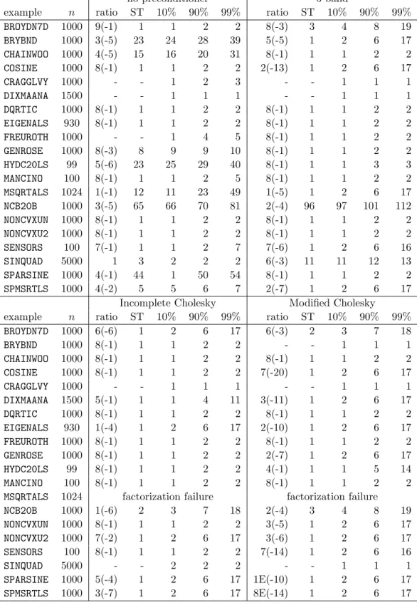
In all of the experiments reported here, the best value found was in fact the optimum value — a factorization of H + λM was used to confirm that the matrix was positive semi-definite, while the algorithm ensured that the remaining optimality conditions hold — although, of course, there is no guarantee that this will always be the case. We measured the iteration (ST) and the percentage (ratio) of the optimal value obtained at the point at which the Steihaug-Toint method left the trust region, as well as the number of iterations taken to achieve 10%, 90% and 99% of the optimal reduction (10%, 90%, 99% respectively).
The results of these experiments are summarized in Table 6.1. In this table we give the name of each example used, along with its dimension n, and the statistics “ratio”(expressed in the form x(y) as a shorthand for x × 10y), “ST”, “10%”, “90%” and “99%” as just described.
Some of the problems had interior solutions, in which case the “ratio” and “ST” statistics are absent (as indicated by a dash). We considered both the unpreconditioned method (M = In),
and a variety of standard preconditioners — a band preconditioner with semi-bandwidth of 5, and modified incomplete and sparse Cholesky factorizations, with the modifications as proposed by Schnabel and Eskow (1991) — used by the LANCELOT package (see, Conn, Gould and Toint, 1992, Chapter 3). The Cholesky factorization methods both failed for the problem MSQRTALS for which the Hessian matrix required too much storage.
We make a number of observations.
1. On some problems, the Steihaug-Toint point gives a model value which is a good approxi-mation to the optimal value.
no preconditioner 5-band
example n ratio ST 10% 90% 99% ratio ST 10% 90% 99%
BROYDN7D 1000 9(-1) 1 1 2 2 8(-3) 3 4 8 19 BRYBND 1000 3(-5) 23 24 28 39 5(-5) 1 2 6 17 CHAINWOO 1000 4(-5) 15 16 20 31 8(-1) 1 1 2 2 COSINE 1000 8(-1) 1 1 2 2 2(-13) 1 2 6 17 CRAGGLVY 1000 - - 1 2 3 - - 1 1 1 DIXMAANA 1500 - - 1 1 1 - - 1 1 1 DQRTIC 1000 8(-1) 1 1 2 2 8(-1) 1 1 2 2 EIGENALS 930 8(-1) 1 1 2 2 8(-1) 1 1 2 2 FREUROTH 1000 - - 1 4 5 8(-1) 1 1 2 2 GENROSE 1000 8(-3) 8 9 9 10 8(-1) 1 1 2 2 HYDC20LS 99 5(-6) 23 25 29 40 8(-1) 1 1 3 3 MANCINO 100 8(-1) 1 1 2 5 8(-1) 1 1 2 2 MSQRTALS 1024 1(-1) 12 11 23 49 1(-5) 1 2 6 17 NCB20B 1000 3(-5) 65 66 70 81 2(-4) 96 97 101 112 NONCVXUN 1000 8(-1) 1 1 2 2 8(-1) 1 1 2 2 NONCVXU2 1000 8(-1) 1 1 2 2 8(-1) 1 1 2 2 SENSORS 100 7(-1) 1 1 2 7 7(-6) 1 2 6 16 SINQUAD 5000 1 3 2 2 2 6(-3) 11 11 12 13 SPARSINE 1000 4(-1) 44 1 50 54 8(-1) 1 1 2 2 SPMSRTLS 1000 4(-2) 5 5 6 7 2(-7) 1 2 6 17
Incomplete Cholesky Modified Cholesky
example n ratio ST 10% 90% 99% ratio ST 10% 90% 99%
BROYDN7D 1000 6(-6) 1 2 6 17 6(-3) 2 3 7 18 BRYBND 1000 8(-1) 1 1 2 2 - - 1 1 1 CHAINWOO 1000 8(-1) 1 1 2 2 8(-1) 1 1 2 2 COSINE 1000 8(-1) 1 1 2 2 7(-20) 1 2 6 17 CRAGGLVY 1000 - - 1 1 1 - - 1 1 1 DIXMAANA 1500 5(-1) 1 1 4 11 3(-11) 1 2 6 17 DQRTIC 1000 8(-1) 1 1 2 2 8(-1) 1 1 2 2 EIGENALS 930 1(-4) 1 2 6 17 2(-10) 1 2 6 17 FREUROTH 1000 8(-1) 1 1 2 2 8(-1) 1 1 2 2 GENROSE 1000 8(-1) 1 1 2 2 2(-7) 1 2 6 17 HYDC20LS 99 8(-1) 1 1 2 2 4(-1) 1 1 5 14 MANCINO 100 8(-1) 1 1 2 2 8(-1) 1 1 2 2
MSQRTALS 1024 factorization failure factorization failure
NCB20B 1000 1(-6) 2 3 7 18 2(-4) 3 4 8 19 NONCVXUN 1000 8(-1) 1 1 2 2 3(-5) 1 2 6 17 NONCVXU2 1000 7(-2) 1 2 6 17 3(-6) 1 2 6 17 SENSORS 100 8(-1) 1 1 2 2 7(-14) 1 2 6 16 SINQUAD 5000 - - 2 2 2 - - 1 1 1 SPARSINE 1000 5(-4) 1 2 6 17 1E(-10) 1 2 6 17 SPMSRTLS 1000 3(-7) 1 2 6 17 8E(-14) 1 2 6 17
Table 6.1: A comparison of the number of iterations required to achieve a given percentage of the optimal model value for a variety of preconditioners. See the text for a key to the data.
2. On other problems, a few extra iterations beyond the Steihaug-Toint point pay handsome dividends.
3. Getting to within 90% or even 99% of the best value very rarely requires many more iterations than to find the Steihaug-Toint point.
In conclusion, based on these numbers, we suggest that a good strategy would be to perform a few (say 5) iterations beyond the Steihaug-Toint point, and only accept the improved point if its model value is significantly better (as this will cost a second pass to compute the Lanczos vectors). We shall consider this further in the next section.
6.2 Do better values than Steihaug-Toint imply a better trust-region method?
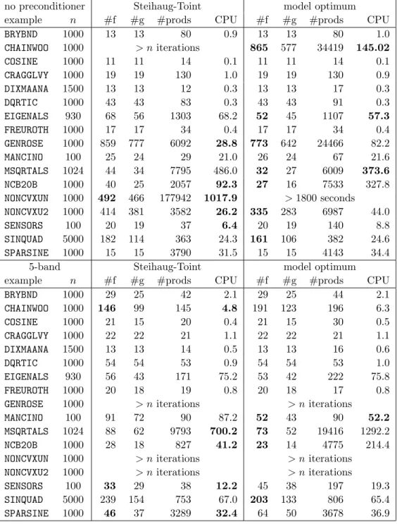
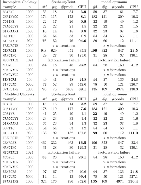
We now consider how the methods we have described for approximately solving the trust-region subproblem perform within a trust-region algorithm. Of particular interest is the question as to whether solving the subproblem more accurately reduces the number of trust-region iterations, or more particularly the cost of solving the problem — the number of iterations is of concern if the evaluation of the objective function and its derivatives is the dominant cost as then there is a direct correlation between the number of iterations and the overall cost of solving the problem. In Tables 6.2 and 6.3, we compare the Steihaug-Toint scheme with the GLTR algorithm (Algorithm 5.1) run to high accuracy. We exclude the problem HYDC20LS for our reported results as no method succeeded in solving the problem in fewer than our limit of n iterations, and the problems BROYDN7D and SPMSRTLS as a number of different local minima were found. In these tables, in addition to the name and dimension of each example, we give the number of objective function (“#f”) and derivative (“#g”) values computed, the total number of matrix-vector products (“#prod”) required to solve the subproblems, and the total CPU time required in seconds. We compare the same preconditioners M as we used in the previous section. We indicate those cases where one or other method performs at least 10% better than its competitor by highlighting the relevant figure in bold.
We observe the following.
1. The use of different M leads to radically different behaviour. Different preconditioners appear to be particularly suited to different problems. Surprisingly, perhaps, the unprecon-ditioned algorithm often performs the best overall.
2. In the unpreconditioned case, the model-optimum variant frequently requires significantly fewer function evaluations than the Steihaug-Toint method. However, the extra algebraic costs per iteration often outweigh the reduction in the numbers of iterations. The advantage in function calls for the other preconditioners is less pronounced.
Ideally, one would like to retain the advantage in numbers of function calls, while reducing the cost per iteration. As we noted in Section 6.1, one normally gets a good approximation to the optimal model value after a modest number of iterations. Moreover, while the Steihaug-Toint point often gives a significantly sub-optimal value, a few extra iterations usually suffices to give
no preconditioner Steihaug-Toint model optimum
example n #f #g #prods CPU #f #g #prods CPU
BRYBND 1000 13 13 80 0.9 13 13 80 1.0 CHAINWOO 1000 > n iterations 865 577 34419 145.02 COSINE 1000 11 11 14 0.1 11 11 14 0.1 CRAGGLVY 1000 19 19 130 1.0 19 19 130 0.9 DIXMAANA 1500 13 13 12 0.3 13 13 17 0.3 DQRTIC 1000 43 43 83 0.3 43 43 91 0.3 EIGENALS 930 68 56 1303 68.2 52 45 1107 57.3 FREUROTH 1000 17 17 34 0.4 17 17 34 0.4 GENROSE 1000 859 777 6092 28.8 773 642 24466 82.2 MANCINO 100 25 24 29 21.0 26 24 67 21.6 MSQRTALS 1024 44 34 7795 486.0 32 27 6009 373.6 NCB20B 1000 40 25 2057 92.3 27 16 7533 327.8 NONCVXUN 1000 492 466 177942 1017.9 > 1800 seconds NONCVXU2 1000 414 381 3582 26.2 335 283 6987 44.0 SENSORS 100 20 19 37 6.4 20 19 140 8.8 SINQUAD 5000 182 114 363 24.3 161 106 382 24.6 SPARSINE 1000 15 15 3790 31.5 15 15 4143 34.4
5-band Steihaug-Toint model optimum
example n #f #g #prods CPU #f #g #prods CPU
BRYBND 1000 29 25 42 2.1 29 25 44 2.1 CHAINWOO 1000 146 99 145 4.8 191 123 196 6.3 COSINE 1000 21 15 20 0.4 21 15 30 0.5 CRAGGLVY 1000 22 22 21 1.1 22 22 21 1.1 DIXMAANA 1500 13 13 14 0.5 13 13 16 0.6 DQRTIC 1000 54 54 53 0.9 54 54 53 1.0 EIGENALS 930 56 43 171 75.2 53 42 222 75.8 FREUROTH 1000 20 18 19 0.8 20 18 17 0.8
GENROSE 1000 > n iterations > n iterations
MANCINO 100 91 72 90 87.2 52 43 90 52.2
MSQRTALS 1024 88 62 9793 700.2 73 52 19416 1292.2
NCB20B 1000 28 18 827 41.2 23 14 4775 214.4
NONCVXUN 1000 > n iterations > n iterations
NONCVXU2 1000 > n iterations > n iterations
SENSORS 100 33 29 38 12.2 45 38 197 19.3
SINQUAD 5000 239 154 753 67.0 203 133 806 65.4
SPARSINE 1000 46 37 3289 32.4 64 50 3678 36.9
Table 6.2: A comparison of the Steihaug-Toint and exact model minimization techniques within a trust-region method, using a variety of preconditioners, for unconstrained minimization (part 1). See the text for a key to the data.
Incomplete Cholesky Steihaug-Toint model optimum
example n #f #g #prods CPU #f #g #prods CPU
BRYBND 1000 55 18 54 3.9 59 37 61 7.7 CHAINWOO 1000 174 115 173 8.1 183 121 309 10.3 COSINE 1000 22 17 26 0.8 22 19 49 1.2 CRAGGLVY 1000 22 22 21 1.5 22 22 21 1.5 DIXMAANA 1500 16 14 15 0.8 32 23 37 1.8 DQRTIC 1000 54 54 53 0.9 54 54 53 1.1 EIGENALS 930 76 52 76 94.6 89 60 112 111.1
FREUROTH 1000 > n iterations > n iterations
GENROSE 1000 948 629 951 35.5 496 322 847 23.5
MANCINO 100 29 27 30 125.0 31 28 32 130.1
MSQRTALS 1024 factorization failure factorization failure
NCB20B 1000 34 18 48 23.2 54 28 150 41.2
NONCVXUN 1000 > n iterations > n iterations
NONCVXU2 1000 > n iterations > n iterations
SENSORS 100 49 41 48 24.8 44 37 136 24.8
SINQUAD 5000 77 52 89 542.6 78 50 121 526.7
SPARSINE 1000 90 75 3465 89.1 135 109 4974 130.3
Modified Cholesky Steihaug-Toint model optimum
example n #f #g #prods CPU #f #g #prods CPU
BRYBND 1000 15 15 14 2.2 59 37 61 7.7 CHAINWOO 1000 178 119 177 7.6 183 121 309 10.3 COSINE 1000 41 25 40 1.1 22 19 49 1.2 CRAGGLVY 1000 23 23 33 1.4 22 22 21 1.6 DIXMAANA 1500 35 23 34 1.3 32 23 37 1.8 DQRTIC 1000 54 54 53 1.2 54 54 53 1.1 EIGENALS 930 133 92 132 167.8 89 60 112 111.0
FREUROTH 1000 > n iterations > n iterations
GENROSE 1000 462 332 463 16.5 496 322 847 23.4
MANCINO 100 31 28 30 129.3 31 28 32 130.1
MSQRTALS 1024 factorization failure factorization failure
NCB20B 1000 38 23 81 26.1 54 28 150 41.2
NONCVXUN 1000 > n iterations > n iterations
NONCVXU2 1000 > n iterations > n iterations
SENSORS 100 97 67 97 40.6 44 37 136 24.8
SINQUAD 5000 14 14 13 99.4 78 50 121 527.1
SPARSINE 1000 324 176 796 852.6 135 109 4974 130.4
Table 6.3: A comparison of the Steihaug-Toint and exact model minimization techniques within a trust-region method, using a variety of preconditioners, for unconstrained minimization (part 2). See the text for a key to the data.
a large percentage of the optimum. Thus, we next investigate both of these issues in the context of an overall trust-region method.
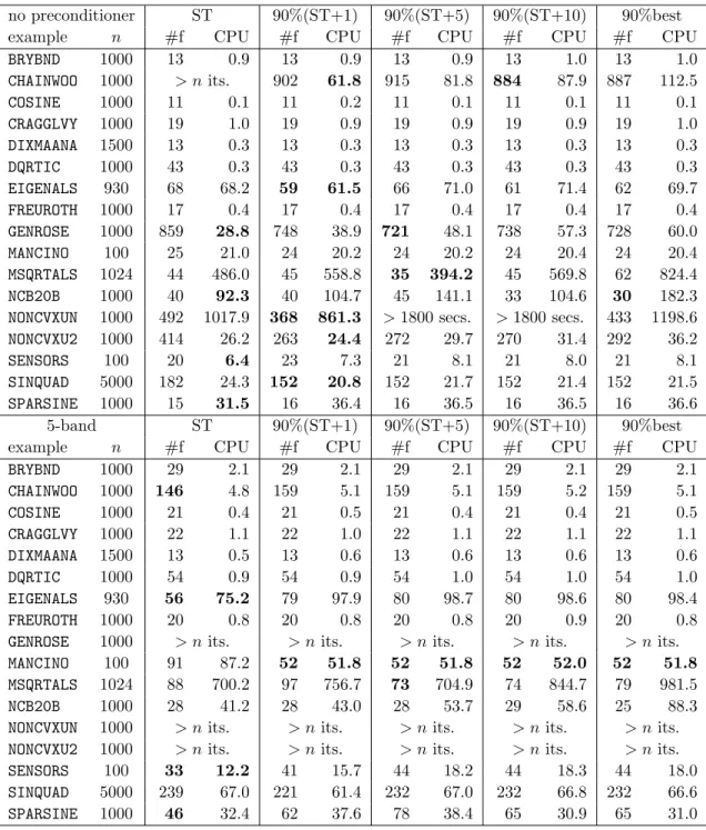
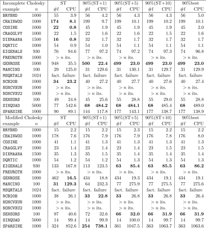
In Tables 6.4 and 6.5, we compare the number of function evaluations (#f), and the CPU time taken to solve the problem for the Steihaug-Toint (“ST”) method with a number of variations on our basic GLTR method (Algorithm 5.1). The basic requirement is that we compute a model value which is at least 90% of the best value found during the first pass of the GLTR method. If this value is obtained by an iterate before that which gives the Toint point, the Steihaug-Toint point is accepted. Otherwise, a second pass is performed to recover the first point at which 90% of the best value was observed. The other ingredient is the choice of the stopping rule for the first pass. One possibility is to stop this pass as soon as the test (6.4) is satisfied. We denote this strategy by “90%best”. The other possibility is to stop when either (6.4) is satisfied or at most a fixed number of iterations beyond the Steihaug-Toint point have occurred. We refer to this as “90%(ST+k)”, where k gives the number of additional iterations allowed. We investigate the cases k = 1, 5 and 10. Once again, we compare the same preconditioners M as we used in the previous section. We highlight in bold those entries which are at least 10% better than the competition.
The conclusions are as broad as before. Each method has its successes and failures, and there is no clear overall best method or preconditioner, although the unpreconditioned version performs surprisingly well. Restricting the number of iteration allowed after the Steihaug-Toint point has been found appears to curb the worst behaviour of the unrestricted method.
no preconditioner ST 90%(ST+1) 90%(ST+5) 90%(ST+10) 90%best
example n #f CPU #f CPU #f CPU #f CPU #f CPU
BRYBND 1000 13 0.9 13 0.9 13 0.9 13 1.0 13 1.0 CHAINWOO 1000 > n its. 902 61.8 915 81.8 884 87.9 887 112.5 COSINE 1000 11 0.1 11 0.2 11 0.1 11 0.1 11 0.1 CRAGGLVY 1000 19 1.0 19 0.9 19 0.9 19 0.9 19 1.0 DIXMAANA 1500 13 0.3 13 0.3 13 0.3 13 0.3 13 0.3 DQRTIC 1000 43 0.3 43 0.3 43 0.3 43 0.3 43 0.3 EIGENALS 930 68 68.2 59 61.5 66 71.0 61 71.4 62 69.7 FREUROTH 1000 17 0.4 17 0.4 17 0.4 17 0.4 17 0.4 GENROSE 1000 859 28.8 748 38.9 721 48.1 738 57.3 728 60.0 MANCINO 100 25 21.0 24 20.2 24 20.2 24 20.4 24 20.4 MSQRTALS 1024 44 486.0 45 558.8 35 394.2 45 569.8 62 824.4 NCB20B 1000 40 92.3 40 104.7 45 141.1 33 104.6 30 182.3
NONCVXUN 1000 492 1017.9 368 861.3 > 1800 secs. > 1800 secs. 433 1198.6
NONCVXU2 1000 414 26.2 263 24.4 272 29.7 270 31.4 292 36.2
SENSORS 100 20 6.4 23 7.3 21 8.1 21 8.0 21 8.1
SINQUAD 5000 182 24.3 152 20.8 152 21.7 152 21.4 152 21.5
SPARSINE 1000 15 31.5 16 36.4 16 36.5 16 36.5 16 36.6
5-band ST 90%(ST+1) 90%(ST+5) 90%(ST+10) 90%best
example n #f CPU #f CPU #f CPU #f CPU #f CPU
BRYBND 1000 29 2.1 29 2.1 29 2.1 29 2.1 29 2.1 CHAINWOO 1000 146 4.8 159 5.1 159 5.1 159 5.2 159 5.1 COSINE 1000 21 0.4 21 0.5 21 0.4 21 0.4 21 0.5 CRAGGLVY 1000 22 1.1 22 1.0 22 1.1 22 1.1 22 1.1 DIXMAANA 1500 13 0.5 13 0.6 13 0.6 13 0.6 13 0.6 DQRTIC 1000 54 0.9 54 0.9 54 1.0 54 1.0 54 1.0 EIGENALS 930 56 75.2 79 97.9 80 98.7 80 98.6 80 98.4 FREUROTH 1000 20 0.8 20 0.8 20 0.8 20 0.9 20 0.8
GENROSE 1000 > n its. > n its. > n its. > n its. > n its.
MANCINO 100 91 87.2 52 51.8 52 51.8 52 52.0 52 51.8
MSQRTALS 1024 88 700.2 97 756.7 73 704.9 74 844.7 79 981.5
NCB20B 1000 28 41.2 28 43.0 28 53.7 29 58.6 25 88.3
NONCVXUN 1000 > n its. > n its. > n its. > n its. > n its. NONCVXU2 1000 > n its. > n its. > n its. > n its. > n its.
SENSORS 100 33 12.2 41 15.7 44 18.2 44 18.3 44 18.0
SINQUAD 5000 239 67.0 221 61.4 232 67.0 232 66.8 232 66.6
SPARSINE 1000 46 32.4 62 37.6 78 38.4 65 30.9 65 31.0
Table 6.4: A comparison of a variety of GLTR techniques within a trust-region method, using a variety of preconditioners, for unconstrained minimization (part 1). See the text for a key to the data.
Incomplete Cholesky ST 90%(ST+1) 90%(ST+5) 90%(ST+10) 90%best
example n #f CPU #f CPU #f CPU #f CPU #f CPU
BRYBND 1000 55 3.9 56 4.2 56 4.3 56 4.3 56 5.0 CHAINWOO 1000 174 8.1 199 9.7 199 10.1 199 10.2 199 10.1 COSINE 1000 22 0.8 45 1.9 45 1.9 45 1.9 45 2.0 CRAGGLVY 1000 22 1.5 22 1.6 22 1.6 22 1.5 22 1.6 DIXMAANA 1500 16 0.8 32 1.7 32 1.7 32 1.7 32 1.7 DQRTIC 1000 54 0.9 54 1.0 54 1.1 54 1.1 54 1.1 EIGENALS 930 76 94.6 77 97.2 74 97.2 74 97.3 74 96.8
FREUROTH 1000 > n its. > n its. > n its. > n its. > n its.
GENROSE 1000 948 35.5 500 22.4 499 23.0 499 23.0 499 23.0
MANCINO 100 29 125.0 31 129.6 31 130.1 31 129.7 31 129.9
MSQRTALS 1024 fact. failure fact. failure fact. failure fact. failure fact. failure
NCB20B 1000 34 23.2 40 27.2 40 27.7 40 27.6 40 27.4
NONCVXUN 1000 > n its. > n its. > n its. > n its. > n its. NONCVXU2 1000 > n its. > n its. > n its. > n its. > n its.
SENSORS 100 49 24.8 45 25.6 55 28.8 55 29.0 55 28.8
SINQUAD 5000 77 542.6 68 484.2 68 484.1 68 485.4 68 489.0
SPARSINE 1000 90 89.1 144 117.8 177 143.1 177 138.7 177 138.9
Modified Cholesky ST 90%(ST+1) 90%(ST+5) 90%(ST+10) 90%best
example n #f CPU #f CPU #f CPU #f CPU #f CPU
BRYBND 1000 15 2.2 15 2.2 15 2.3 15 2.2 15 2.2 CHAINWOO 1000 178 7.6 176 7.9 176 7.9 176 7.8 176 8.0 COSINE 1000 41 1.1 41 1.3 41 1.3 41 1.3 41 1.3 CRAGGLVY 1000 23 1.4 23 1.4 23 1.4 23 1.5 23 1.5 DIXMAANA 1500 35 1.3 35 1.5 35 1.4 35 1.4 35 1.4 DQRTIC 1000 54 1.2 54 1.2 54 1.3 54 1.3 54 1.3 EIGENALS 930 133 167.8 113 123.5 63 85.4 63 85.5 63 86.2
FREUROTH 1000 > n its. > n its. > n its. > n its. > n its.
GENROSE 1000 462 16.5 434 18.8 434 19.3 434 19.1 434 19.1
MANCINO 100 31 129.3 64 232.3 77 275.9 77 275.5 77 275.6
MSQRTALS 1024 fact. failure fact. failure fact. failure fact. failure fact. failure
NCB20B 1000 38 26.1 33 22.8 33 26.8 33 26.8 33 26.4
NONCVXUN 1000 > n its. > n its. > n its. > n its. > n its. NONCVXU2 1000 > n its. > n its. > n its. > n its. > n its.
SENSORS 100 97 40.6 72 32.6 66 32.0 66 31.9 66 31.9
SINQUAD 5000 14 99.4 14 99.9 14 100.0 14 99.7 14 99.7
SPARSINE 1000 324 852.6 254 738.1 361 1047.5 363 1063.7 363 1063.6
Table 6.5: A comparison of a variety of GLTR techniques within a trust-region method, using a variety of preconditioners, for unconstrained minimization (part 2). See the text for a key to the data.
7
Perspectives and conclusions
We have considered a number of methods which aim to find a better approximation to the solution of the trust-region subproblem than that delivered by the Steihaug-Toint scheme. These methods are based on solving the subproblem within a subspace defined by the Krylov space generated by the conjugate-gradient and Lanczos methods. The Krylov subproblem has a number of useful properties which lead to its efficient solution. The resulting algorithm is available as a Fortran 90 module, HSL VF05, within the Harwell Subroutine Library (1998).
We must admit to being slightly disappointed that the new method did not perform uniformly better than the Steihaug-Toint scheme, and were genuinely surprised that a more accurate ap-proximation does not appear to significantly reduce the number of function evaluations within a standard trust-region method, at least in the tests we performed. While this may limit the use of the methods developed here, it also calls into question a number of other recent eigensolution-based proposals for solving the trust-region subproblem (see Rendl, Vanderbei and Wolkowicz, 1995, Rendl and Wolkowicz, 1997, Sorensen, 1997, Santos and Sorensen, 1995). While these authors demonstrate that their methods provide an effective means of solving the subproblem, they make no effort to evaluate whether this is actually useful within a trust-region method. The results given in this paper suggest that this may not in fact be the case. This also leads to the interesting question as to whether it is possible to obtain useful low-accuracy solutions with these methods. We believe that further testing is needed to confirm the trends we have observed here. We should not pretend that the formulae given in this paper are exact or even accurate in floating-point arithmetic. Indeed, it is well-known that the floating-point matrices Qk from
the Lanczos method quickly loose M -orthonormality (see, for instance, Parlett, 1980, Section 13.3). Despite this, the method as given appears to be capable of producing usable approximate solutions to the trust-region subproblem. We are currently investigating why this should be so.
One further possibility, which we have not considered so far, is to find an estimate λ using the first pass of Algorithm 5.1, and then to compute the required s by minimizing the uncon-strained model hg, si + 1
2hs, (H + λM)si using the preconditioned conjugate gradient method.
The advantage of doing this is that any instability in the first pass does not necessarily reappear in this auxiliary calculation. The disadvantages are that it may require more work than simply using (5.1), and that λ must be computed sufficiently large to ensure that H + λM is positive semi-definite.
Acknowledgement
We would like to thank John Reid for his helpful advice on computing eigenvalues of tridiagonal matrices, and Jorge Mor´e for his useful comments on the Mor´e and Sorensen (1983) method. Many thanks are also due to Jorge Nocedal and two anonymous referees. We are grateful to the British Council-MURST for a travel grant (ROM/889/95/53) which made some of this research possible.
References
I. Bongartz, A. R. Conn, N. I. M. Gould, and Ph. L. Toint. CUTE: Constrained and unconstrained testing environment. ACM Transactions on Mathematical Software, 21(1), 123–160, 1995. R. H. Byrd, R. B. Schnabel, and G. A. Schultz. A family of trust-region-based algorithms for
unconstrained minimization with strong global convergence properties. SIAM Journal on Numerical Analysis, 22(1), 47–67, 1985.
A. R. Conn, N. I. M. Gould, and Ph. L. Toint. LANCELOT: a Fortran package for large-scale nonlinear optimization (Release A). Number 17 in ‘Springer Series in Computational Math-ematics’. Springer Verlag, Heidelberg, Berlin, New York, 1992.
J. E. Dennis and H. H. W. Mei. Two new unconstrained optimization algorithms which use function and gradient values. Journal of Optimization Theory and Applications, 28(4), 453– 482, 1979.
D. M. Gay. Computing optimal locally constrained steps. SIAM Journal on Scientific and Statistical Computing, 2, 186–197, 1981.
S. M. Goldfeldt, R. E. Quandt, and H. F. Trotter. Maximization by quadratic hill-climbing. Econometrica, 34, 541–551, 1966.
Harwell Subroutine Library. A catalogue of subroutines (release 13). AEA Technology, Harwell, Oxfordshire, England, 1998. To appear.
M. D. Hebden. An algorithm for minimization using exact second derivatives. Technical Report T. P. 515, AERE Harwell Laboratory, Harwell, UK, 1973.
S. Lucidi and M. Roma. Numerical experience with new truncated Newton methods in large scale unconstrained optimization. Computational Optimization and Applications, 7(1), 71– 87, 1997.
J. J. Mor´e and D. C. Sorensen. Computing a trust region step. SIAM Journal on Scientific and Statistical Computing, 4(3), 553–572, 1983.
S. G. Nash. Newton-type minimization via the Lanczos method. SIAM Journal on Numerical Analysis, 21(4), 770–788, 1984.
B. N. Parlett. The Symmetric Eigenvalue Problem. Prentice-Hall, Englewood Cliffs, New Jersey, 1980.
B. N. Parlett and J. K. Reid. Tracking the progress of the Lanczos algorithm for large symmetric eigenproblems. Journal of the Institute of Mathematics and its Applications, 1, 135–155, 1981.
M. J. D. Powell. A new algorithm for unconstrained optimization. In J. B. Rosen, O. L. Man-gasarian and K. Ritter, eds, ‘Nonlinear Programming’, Academic Press, London and New York, 1970.
M. J. D. Powell. Convergence properties of a class of minimization algorithms. In O. L. Man-gasarian, R. R. Meyer and S. M. Robinson, eds, ‘Nonlinear Programming, 2’, Academic Press, London and New York, 1975.
F. Rendl and H. Wolkowicz. A semidefinite framework for trust region subproblems with appli-cations to large scale minimization. Mathematical Programming, Series B, 77(2), 273–299, 1997.
F. Rendl, R. J. Vanderbei, and H. Wolkowicz. Max-min eigenvalue problems, primal-dual interior point algorithms, and trust region subproblems. Optimization Methods and Software, 5(1), 1– 16, 1995.
S. A. Santos and D. C. Sorensen. A new matrix-free algorithm for the large-scale trust-region subproblem. Technical Report TR95-20, Department of Computational and Applied Math-ematics, Rice University, Houston, Texas, USA, 1995.
R. B. Schnabel and E. Eskow. A new modified Cholesky factorization. SIAM Journal on Scientific Computing, 11, 1136–1158, 1991.
D. C. Sorensen. Newton’s method with a model trust modification. SIAM Journal on Numerical Analysis, 19(2), 409–426, 1982.
D. C. Sorensen. Minimization of a large-scale quadratic function subject to a spherical constraint. SIAM Journal on Optimization, 7(1), 141–161, 1997.
T. Steihaug. The conjugate gradient method and trust regions in large scale optimization. SIAM Journal on Numerical Analysis, 20(3), 626–637, 1983.
Ph. L. Toint. Towards an efficient sparsity exploiting Newton method for minimization. In I. S. Duff, ed., ‘Sparse Matrices and Their Uses’, Academic Press, London and New York, 1981.