HAL Id: tel-01925862
https://tel.archives-ouvertes.fr/tel-01925862
Submitted on 18 Nov 2018HAL is a multi-disciplinary open access archive for the deposit and dissemination of sci-entific research documents, whether they are pub-lished or not. The documents may come from teaching and research institutions in France or abroad, or from public or private research centers.
L’archive ouverte pluridisciplinaire HAL, est destinée au dépôt et à la diffusion de documents scientifiques de niveau recherche, publiés ou non, émanant des établissements d’enseignement et de recherche français ou étrangers, des laboratoires publics ou privés.
phenomenon in PWR steam generators - understanding
and prioritization of its formation mechanisms
Guangze Yang
To cite this version:
Guangze Yang. Investigations of the Tube Support Plate (TSP) clogging phenomenon in PWR steam generators - understanding and prioritization of its formation mechanisms. Chemical Physics [physics.chem-ph]. Université Pierre et Marie Curie - Paris VI, 2017. English. �NNT : 2017PA066441�. �tel-01925862�
ED388 / IRCP Chimie ParisTech
Investigations of the Tube Support Plate (TSP) clogging
phenomenon in PWR steam generators – understanding and
prioritization of its formation mechanisms
Par Guangze YANG
Thèse de doctorat de chimie physique et chimie analytique
Dirigée par Alexandre CHAGNES
Présentée et soutenue publiquement le 16 Novembre 2017
Devant un jury composé de :
Didier Devilliers, Université Pierre et Marie Curie, Paris, Président Gilles Berger, Université de Toulouse III, Toulouse, Rapporteur Nicolas Marmier, Université Nice Sophia Antipolis, Nice, Rapporteur Isabelle Mabille, Université Pierre et Marie Curie, Paris, Examinateur
Etienne Tevissen, CEA, Cadarache, Invité Sophie Delaunay, EDF, Renardières, Invité
Veronique Pointeau, CEA, Cadarache, Encadrante (co-direction) Alexandre Chagnes, Université de Lorraine, Nancy, Directeur de thèse
It gives me immense pleasure to write this note of acknowledgement for everyone who has been involved with this project in one way or the other.
First and foremost I want to thank my CEA supervisor Véronique. Pointeau. It has been an honour to be your first PhD student. I appreciate all your contributions of time and ideas to make my PhD experience productive and stimulating. The joy and enthusiasm you have for the research was contagious and motivational for me. I wholeheartedly thank you for the constant support and encouragement, both personally and professionally, during the entire duration of my PhD.
I take this opportunity to thank Alexandre. Chagnes (Université de Lorraine) for agreeing to be my thesis director and your constant guidance throughout. Your time and effort in helping me well adapt the thesis approaches and improving my scientific redaction have been invaluable. I am also thankful for your precious implications in the obtainment of my future researcher position in the IFCEN. I would like to thank Etienne. Tevissen (CEA), for welcoming me on April, 2014 in Cadarache for the thesis interview and accepting me as a PhD student. Your guidance on the development of my thesis was constant and useful during all these three years.
I would like to thank all the jury members for your presence, your suggestions to improve the manuscript and your pertinent questions and comments on the day of my defence.
I want to thank, Huber Catelette (EDF), Gérard Côte (Chimie ParisTech), Philippe Moisy (CEA) and François Paquet (IRSN), for recommending me for this PhD position.
I want to thank my laboratory (LHC) chief in CEA, Isabelle Tkatshenko, for supporting me to present my PhD work in various French and international conferences. Thank you, Isabelle Mounet and Gaëlle Pestel, for solving administrative issues to facilitate ma participation in these conferences. Thank you Alexandre, Véronique and Etienne once again for encouraging me to participate to conferences and reviewing my proceedings, as well as journal articles.
Thanks to members of COLENTEC team in LHC, Patricia. Schindler, Yves. Philibert, Isabelle. Holveck, Stéphane. Bantiche, Pascal. Marand, Jean-Philippe. Descamps and Véronique. Pointeau, for successfully performing this highly complicated experiment. Particular thanks go to Yves and Isabelle. H, for helping me establish the security file for autoclave tests and launch each campaign. It was an immense pleasure to work in this enthusiast team.
I take this opportunity to thank the team in the University of Manchester, particularly Fabio. Scenini and Stefano. Cassineri, for your agreement of establishing our collaboration in electrokinetic investigations. I am also thankful for your welcome during my stay in Manchester. Your insight on electrokinetic phenomenon has been highly appreciated.
Thank you, Frédéric Rey and Serge Delafontaine (CEA), for providing me the modelling of the fluid for the interpretation of electrokinetic results. I appreciate your precious contributions of time and ideas. I would like to thank Martiane. Cabié (Université Aix-Marseille), for your contributed time and efforts during my TEM characterizations. Your suggestions and advice were useful for the analysis of results. My sincere thanks to Brigitte. Thormos of LIPC (CEA) for your helps in SEM sample preparation and observation. Thank you Véronique for sharing with me your insight on SEM/TEM characterizations. I want to thank Phillipe Barboux, Domitille Giaume, Phillipe Marcus and Cédric Guyon (Chimie ParisTech) for the initial intention of collaboration.
Bhattacharjee, Brice. Bourdeaux and Corentin. Bouzet for the wonderful time spent together.
My sincere thanks go to Alexandre, Véronique and Etienne for correcting and improving the present manuscript. This work would not have been possible without your dynamic and efficient corrections. I would like to thank my parents for your support at every stage of my life. I am also thankful for my friends in Aix en Provence for the amazing three years spent together.
This thesis has been the combined effort of so many people, Véronique, Alexandre, Etienne, my family and friends…
The steam generator is an essential component in PWR which allows the heat exchange between the primary and secondary circuits. After 15-20 years of functioning, an obstruction by deposits of flow holes between Tube Support Plate (TSP) and primary tubes is observed, called TSP clogging. This phenomenon may lead to dramatic consequences for nuclear power plant operation and may be responsible for safety issues. The aim of this thesis is to deepen, experimentally and numerically, the understanding of the mechanisms responsible for TSP clogging by identifying and prioritizing the preponderant processes.
COLENTEC is an experimental facility designed to reproduce TSP clogging deposits under representative conditions of the upper part of steam generators. Microscopic characterizations (SEM and TEM) allowed revealing the deposit formation by precipitation and the initiation role of material passivation in deposit formation. Lipping and ripple forms, specifying TSP clogging, were not observed in COLENTEC tests. This is suggested to be caused by insufficient concentration of suitable particles at the test section. Particle deposition is supposed to be essential for the formation of lipping deposits at the inlet of TSP.
Electrokinetic and flashing phenomena are supposed to contribute to TSP clogging formation, having cementing effects on the deposits initially formed by particle deposition. An experimental collaboration program with the University of Manchester was established to better understand the clogging formation by investigating the role of electrokinetic phenomenon. This study allowed reforming deposits with lipping and ripple forms as observed in EDF steam generators. Electrokinetic involvement, strongly affected by flow velocity, was considerably suggested in TSP clogging formation.
Numerical quantification of deposit formation by particle deposition, flashing and electrokinetic phenomenon was performed and compared to EDF feedbacks on TSP clogging formation. Electrokinetic phenomenon was found to play a predominant role, whereas particle deposition was suggested to have a minor contribution to clogging formation.
Key words: clogging, magnetite, precipitation, particle deposition, electrokinetic, mechanism prioritization, experimental deposit rebuild-up, calculation.
Contents ... vi
List of Figures ... ix
List of Tables ... xv
Nomenclature ... 1
Introduction ... 6
Chapter 1 State of the art ... 8
1.1 Introduction ... 8
1.2 PWR secondary circuit... 8
1.2.1 General description ... 8
1.2.2 Recirculating steam generator ... 9
1.2.3 Thermohydraulics in PWR steam generator ... 11
1.2.3.1 Two-phase flow fundamentals ... 11
1.2.3.1.1 Two-phase flow system basic notions ... 11
1.2.3.1.2 Two-phase flow patterns ... 13
1.2.3.2 Thermohydraulics of 51B type steam generators ... 14
1.2.4 Materials used in the secondary circuit ... 14
1.2.5 PWR secondary flow chemistry ... 15
1.2.6 Corrosion phenomena in PWR secondary circuit ... 16
1.2.6.1 Stress corrosion cracking (SCC) ... 16
1.2.6.2 General corrosion and Flow accelerated corrosion (FAC)... 17
1.2.6.3 Parameters affecting flow accelerated corrosion – TSP clogging source ... 18
1.2.6.3.1 Effects of pH and temperature – magnetite solubility ... 18
1.2.6.3.2 Effect of oxygen concentration ... 19
1.2.6.3.3 Effect of material composition ... 20
1.2.6.3.4 Effect of thermohydraulics ... 22
1.3 Properties of magnetite particle ... 23
1.3.1 Structural property ... 24
1.3.2 Magnetite surface charge ... 25
1.3.2.1 Electrical double layer (EDL) ... 25
1.3.2.2 Zeta potential ... 26
1.3.2.3 Surface characterizations of magnetite ... 27
1.4 Steam generator degradation phenomena ... 27
1.4.1 Tube fouling ... 28
1.4.2 Tube Support Plate clogging ... 29
1.4.2.2.2 Wide Range Level (WRL) monitoring in stationary regime ... 30
1.4.2.2.3 Eddy current inspection ... 30
1.4.2.3 NPP feedbacks of TSP clogging ... 30
1.4.2.4 Current countermeasures ... 32
1.5 Phenomenology of TSP clogging formation ... 32
1.5.1 Magnetite particle deposition ... 33
1.5.1.1 Previous experimental studies ... 33
1.5.1.2 Magnetite particle deposition models ... 34
1.5.1.2.1 Transport step ... 35 1.5.1.2.2 Attachment step ... 38 1.5.2 Surface precipitation ... 39 1.5.2.1 Attainment of solubility ... 39 1.5.2.2 Formation of nuclei ... 39 1.5.2.3 Growth of crystals ... 40
1.5.3 Specific TSP clogging formation mechanisms at the inlet of TSP ... 41
1.5.3.1 Vena contracta mechanism ... 42
1.5.3.2 Flashing ... 44
1.5.3.3 Results of modelling study comprising vena contracta and flashing ... 45
1.5.3.4 Electrokinetics ... 45
1.6 Conclusions of Chapter 1 ... 48
Chapter 2 Experimental investigation of TSP clogging phenomenon ... 49
2.1 Introduction ... 49
2.2 Representative experiments ... 49
2.2.1 Global deposit build-up tool under representative conditions: COLENTEC facility ... 50
2.2.2 COLENTEC – 2015 experimental conditions ... 52
2.2.3 Materials used for COLENTEC test ... 54
2.2.4 Characterization results of COLENTEC-2015 samples... 55
2.2.4.1 Optical and SEM observations ... 56
2.2.4.2 TEM investigations ... 59
2.2.4.2.1 Characterization of titanium thin section ... 59
2.2.4.2.2 Characterization of stainless steel thin section ... 64
2.3 Simulated experiments ... 70
2.3.1 Description of autoclave tests ... 70
2.3.2 Iron incorporation into stainless steel corrosion layer ... 72
2.3.3 Ti/SS galvanic corrosion effects ... 74
2.4 Conclusions of Chapter 2 ... 75 Chapter 3 Specific experimental investigation of deposit build-up by electrokinetic phenomenon
electrokinetic deposit build-up ... 78
3.3 Experimental system ... 79
3.4 Experimental conditions ... 81
3.5 Results ... 83
3.5.1 Morphology and characterization of the deposits ... 83
3.5.2 Deposit build-up rates ... 92
3.6 Discussions ... 93
3.6.1 Effect of flow velocity ... 93
3.6.2 Comparisons with COLENTEC results and EDF observations ... 98
3.7 Conclusions of Chapter 3 ... 100
Chapter 4 Numerical investigation of TSP clogging phenomenon ... 102
4.1 Introduction ... 102
4.2 Hypotheses and input data ... 103
4.2.1 Hypotheses ... 103
4.2.2 Input data ... 104
4.3 Results ... 105
4.3.1 Phenomenon prioritization with different particle sizes ... 105
4.3.2 Phenomenon prioritization with different total iron concentrations ... 107
4.4 Discussions ... 108
4.5 Conclusions of Chapter 4 ... 109
Chapter 5 Overall conclusions and perspectives ... 110
References ... 115
Appendix A Scanning Electronic Microscope ... 130
Appendix B Transmission Electronic Microscope ... 131
Figure 1.1: Scheme of PWR secondary circuit (Pressurized Water Reactor Systems, n.d.). ... 9 Figure 1.2: Scheme of 51B-type PWR recirculating steam generator (Bodineau and Sollier, 2013; Girard et al., 2013). TSP clogging phenomenon is observed after several decades of operation and is represented at the top right. ... 10 Figure 1.3: Two-phase flow patterns’ sequence as a function of steam quality x (K. Popov, 2015). “G” and “L” represents the vapour phase and the liquid phase, respectively. ... 13 Figure 1.4: Pourbaix diagram of iron calculated with PHREEPLOT, using the Lawrence Livermore National Laboratory (llnl) database (“llnl.dat”, n.d.). Temperature = 200 °C corresponding to the temperature of the secondary circuit before entering into the SG; pH25 °C > 9 corresponds to pH200 °C > 6
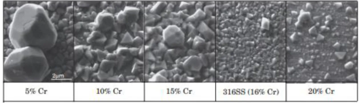
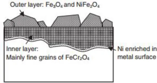
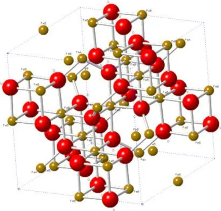
(Yang et al., 2017a); Potential Eh in Volt given vs. the Standard Hydrogen Electrode (SHE). Red point indicates that the stable form of iron is magnetite under the above-mentioned conditions. ... 17 Figure 1.5: Magnetite solubility as a function of temperature and pH at 25 °C. pH was conditioned by adding ammonia at 0.1 ppm to 2.0 ppm. A maximum of magnetite solubility is observed at about 150 °C whatever the pH values. Detailed data cannot be provided. (Unpublished EPRI results) ... 19 Figure 1.6: SEM images of the oxide film after immersion in simulated PWR primary water at 320 °C for 380 h, observed by Terachi’s investigation (Terachi et al., 2008). ... 20 Figure 1.7: Schematic image of cross-sectional oxide film on stainless steel, proposed by Terachi’s work (Terachi et al., 2008). ... 21 Figure 1.8: Electron diffraction patterns of the inner layer in 5% Cr, 10% Cr and 16% Cr after immersion in simulated PWR primary water at 320 °C for 380 h, obtained by Terachi’s investigation (Terachi et al., 2008). ... 21 Figure 1.9: Observed double-layer structure for HCM12A sample exposed for eight weeks in supercritical water conditions. Iron and chromium evolutions are shown, which highlight chromium enrichment in the inner corrosion layer (Bischoff et al., 2012). ... 22 Figure 1.10: Photo of a magnetite mineral from Bolivia (Wikipedia source). Bipyramid crystals are observed. ... 23 Figure 1.11: Structure of magnetite. Red spheres represent O2-; marron spheres represent the ferrous
and ferric ions. FeA (ferric ions) occupy tetrahedral sites and FeB (ferric and ferrous ions) occupy octahedral sites. ... 24 Figure 1.12: Potential variation across the EDL. The potential between the surface and IHP, as well as the IHP and the OHP varies linearly and then exponentially in the diffuse layer. Ψ0, Ψi and Ψd represent
the wall potential, IHP potential and OHP potential respectively. A shear plane is placed with a distance of dek from the wall. ϛ represents the corresponding potential at this plane, named zeta potential. ... 26
Figure 1.13: Photo of SG tube fouling (Prusek, 2012). ... 28 Figure 1.14: Photo of TSP clogging: top view of a “clean” quatrefoil flow hole (a); almost fully clogged quatrefoil flow hole (b) (Prusek et al., 2013; adapted by Yang et al., 2017a). Lipping form and ripple form are observed for clogged flow hole. ... 29
Figure 1.17: Pattern of vena contracta region (Prusek, 2012; Prusek et al., 2013). ... 43 Figure 1.18: Top view of a pattern of a TSP (secondary flow hole in white colour). ... 44 Figure 1.19: Illustration of magnetite formation due to electrokinetic phenomena onto TSP. iw represents
the wall current; is represents the streaming current. ... 46
Figure 1.20: The proposed electrokinetic mechanism of deposit propagation along the annulus of a flow-restriction (Guillodo et al., 2012). ... 47 Figure 2.1: Flowsheet of the COLENTEC test loop. ... 50 Figure 2.2: Photo of COLENTEC primary loop (a), COLENTEC air cooler (b), and COLENTEC CVCS system (c). ... 51 Figure 2.3: Photo of COLENTEC secondary loop (a), COLENTEC test section (b) with four primary SG tubes maintained by a titanium TSP (the COLENTEC secondary fluid circulates in the quatrefoils between the tubes and TSP) and COLENTEC titanium TSP with removable test coupons inserted in the dedicated sites (c). ... 51 Figure 2.4: Evolution of the temperature in the test section (1), at the inlet (2) and the outlet of the condenser (3) and at the inlet of the secondary boiler (4) in COLENTEC-2015-1 test from the 24th
February to the 4th March 2015. ... 52
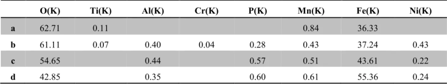
Figure 2.5: Evolution of the temperature during the COLENTEC-2015-2 test. (1): temperature in the test section; (2): temperature at the inlet; (3): temperature at the outlet of the condenser; (4): temperature at the inlet of the secondary boiler. ... 53 Figure 2.6: Photo of COLENTEC test coupons made of titanium (Ti), stainless steel (SS) and mirror-polished titanium (M-Ti) (a); Scheme of COLENTEC test coupons (b). A specific ergot is implemented for the TSP fixation and the coupon surface is curved to satisfy the real geometric configuration of TSP flow hole; Scheme of COLENTEC test coupons (c). Both titanium and stainless steel test coupons have a length of 30 mm, a maximal width of 7.19 mm and an equally-curved surface; Photo of the titanium TSP with 16 test coupons inserted for COLENTEC-2015-1 (d). ... 55 Figure 2.7: Surface morphology observed by secondary electron mode SEM of titanium test coupon after 11 days under experimental conditions of COLENTEC-2015-1. A depleted-deposit region is observed at the inlet of TSP. ... 56 Figure 2.8: Comparison between a titanium (Ti) test coupon and a mirror-polished titanium (M-Ti) coupon after 11 days under experimental conditions of COLENTEC-2015-1. Ti sample after 11 days appears to be covered by a homogenous black layer, which contains majorly iron and oxygen (measured by EDS); M-Ti coupon appears unchanged. ... 57 Figure 2.9: Surface morphology observed by secondary electron mode SEM of titanium test coupon after 11 days under experimental conditions of COLENTEC-2015-1 (a) and after 63 days under experimental conditions of COLENTEC-2015-2 (b). Iron oxide crystal twinning is observed in both cases. Crystal size is estimated to be around 1 µm after 11 days (a), and 5 µm after 63 days (b). ... 57 Figure 2.10: SEM picture in Back-scattered electron mode of stainless steel cut coupon obtained during the COLENTEC-2015-2 test (a) and titanium cut coupon obtained during the COLENTEC-2015-2 test (b). ... 58 Figure 2.11: Thin section of titanium sample (a). Three principal areas are observed: (1): area close to titanium substrate; (2): porous layer; (3): compact layer; Zoom close to titanium substrate (b). White lines delimit a porous layer of around 100 nm, which is supposed to be the corrosion layer mainly composed of titanium and oxygen. ... 59 Figure 2.12: Seven different EDS analyses of titanium sample obtained during COLENTEC 2015 test in the area close to Ti substrate (a); High resolution (HR) TEM image (b) of a particle from #2 region in Figure 2.12a (white dash line represents the border of a particle present in this layer). ... 60
separated by the yellow dash line and iron particles. Only the evolution of each element is intended to be shown along the white line, comparisons between different elements are not significant. ... 61 Figure 2.14: EDS mapping of the closed titanium area, containing titanium substrate, TiO2 corrosion
layer, potential solid solution layer and deposited iron particles, showing the TEM image and mapping zone (a); and element distribution of iron (b), titanium (c), oxygen (d) and manganese (e). ... 62 Figure 2.15: EDS mapping of a zoomed close titanium area, containing TiO2 corrosion layer, the two
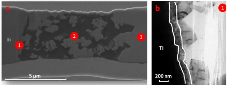
potential solid solution layers and deposited iron particles, showing the TEM image and mapping zone and element distribution of iron, titanium, oxygen and manganese... 62 Figure 2.16: Surface TEM and EDS analysis of porous and external compact layer in the titanium sample obtained during the COLENTEC 2015 test (a). The EDS analyses were performed under the same conditions in the four red areas shown in the TEM image; Diffraction patterns (b) of a area in Figure 2.16a. ... 63 Figure 2.17: EDS mapping of a selected area of the compact layer of the titanium thin section. ... 64 Figure 2.18: Pictures by TEM in the bright field (BF) mode of the thin section of stainless steel sample obtained during the COLENTEC 2015 test (a). Three different layers are observed: (1) Compact inner corrosion layer delimited by an outer-inner layer interface (white dash line), (2) Compact outer corrosion layer and (3) Particle aggregation; Specific TEM BF observation of particle aggregation (b) (Particles size is of about several hundreds of nm). ... 65 Figure 2.19: Surface TEM and EDS analysis of stainless steel sample obtained during the COLENTEC-2015 test. (a) stainless steel material; (b) inner corrosion layer; (c) and (d) outer corrosion layer; (e) particle aggregation. The EDS analysis was performed under same conditions in the five red areas (see composition in Table 2.7). ... 66 Figure 2.20: Indicator of different regions where analyses are performed (a); Diffraction patterns of b area (b); Diffraction patterns of c area (c); Diffraction patterns of d area (d); High resolution (HR) TEM image of a particle from e area (white dash line represents the border of a particle present in this layer) (e). ... 67 Figure 2.21: EDS analyses performed along the white line in images (a), (b) and (c). Only the evolution of each element is intended to be shown along the white line. Comparisons between different elements are not significant. ... 68 Figure 2.22: EDS mapping of the interface area between particle aggregation layer and outer corrosion layer, showing the TEM image and mapping zone (a); and element distribution of iron (b), chromium (c) and oxygen (d). A thin chromium (around 100 nm) enriched layer is observed at the outermost corrosion layer and delimited by white line in (c). ... 69 Figure 2.23: Photo of autoclave system. ... 71 Figure 2.24: Scheme of the test coupon designed especially for autoclave to investigate galvanic corrosion. Green coupon is made of stainless steel inserted into the pre-machined titanium coupon coloured in grey. ... 71 Figure 2.25: SEM observation of the SS coupon in the Autoclave-A (Ti-SS-Ti sample) after an immersion during one month at 250 °C and 30 bars without iron in the autoclave (a). A corrosion layer of 2 µm containing iron, oxygen, silicon, aluminium and chromium is observed; SEM observation of the SS coupon in the Autoclave-B (Ti-SS-Ti sample) after an immersion during one month in an autoclave containing 5 ppb of iron (b). A corrosion layer of 6 µm containing iron, oxygen, silicon, aluminium and chromium is observed. ... 73 Figure 2.26: SEM observation of the surface of SS coupon in the Autoclave-C (Ti-SS-Ti sample) after ten days of immersion at 250 °C and 30 bars in autoclave without iron (a). No corrosion layer is observed; SEM observation of the surface of SS coupon in the Autoclave-D (Ti-SS-Ti sample) after ten days of immersion in the presence of 5 ppb of iron in the autoclave (b). A corrosion layer of 5 µm containing iron, oxygen, silicon, aluminium and chromium is observed. ... 73
Figure 3.2: Scheme of the recirculating stainless steel autoclave at the University of Manchester fitted with a flow cell (2) which could be activated by opening the flow cell valve (3) (McGrady et al., 2017). ... 80 Figure 3.3: Photos of the recirculating autoclave containing the flow cell (a) and feed tanks (b); Geometry of the flow cell inside the autoclave vessel (c). ... 81 Figure 3.4: Scheme of titanium discs used for studying the deposit build-up during test at the University of Manchester... 81 Figure 3.5: Secondary electron mode SEM pictures (left column) and 3D visualisations obtained by laser confocal microscopy measurements (right column) of front face of disc 1 (4 m/s (a)), disc 2 (8 m/s (b)) and disc 3 (18 m/s (c)) after electrokinetic tests. Yellow dash circles show the location where deposit formation starts onto the surface of discs 2 and 3. ... 85 Figure 3.6: Magnified secondary electron mode SEM images of the surface deposits on (left) disc 1 (4 m/s) and (right) disc 2 (8 m/s). Deposits containing iron and oxygen follow the flow direction. ... 86 Figure 3.7: Magnified secondary electron mode SEM images of the surface deposits of disc 3 (18 m/s). Deposits containing iron and oxygen seem to be less porous than that formed on discs 1 and 2. No preferred direction is observed for the deposit formation. ... 86 Figure 3.8: Magnified secondary electron mode SEM images of the inlet of disc 1 (4 m/s (a)), disc 2 (8 m/s (b)) and disc 3 (18 m/s (c)); EDS profile analysis of a line crossing the orifice of disc 3, indicating the formation of iron oxide on the edge of the orifice (d). ... 87 Figure 3.9: SEM images of the inner surface of disc 1 (4 m/s (a)) and disc 2 (8 m/s (b)). Negligible deposits are present onto the inner surface at the entrance region. For disc 1, hydrodynamically controlled deposits appear to be formed on the inner surface at about 150 µm from the orifice edge. 87 Figure 3.10: Secondary electron mode SEM image of disc 3 (a) showing the formation of deposits on the edge of orifice (radial BUR) and a general view of the inner surface near the orifice inlet; magnified visualisation of the inner surface of disc 3 (b), indicating the formation of ripples containing iron oxide. ... 88 Figure 3.11: Secondary electron mode SEM pictures (left column) and 3D visualisations obtained by laser confocal microscopy measurements (right column) of front face of disc 4 (a) and disc 5 (b) after electrokinetic tests. Red dash circle represents the initial orifice edge, overlapped by deposits for disc 4. ... 89 Figure 3.12: SEM image (secondary electron mode) of the outer deposit layer onto disc 4 in which deposits appear to follow the flow (a); SEM image of the intermediate deposit layer which is less porous than the outer layer (flow-perpendicular ripples containing iron and oxygen are observed) (b). ... 89 Figure 3.13: Observation of two important circular ripples containing iron and oxygen on the initial edge of the orifice of disc 4. ... 90 Figure 3.14: SEM image (secondary electron mode) of the inner deposit layer observed within the orifice of the disc 4 where faceted particles can be observed (a); SEM image of particles present in this layer (b), which contain iron, chromium and oxygen (size of these particles can reach 15 µm). ... 90 Figure 3.15: EDS mapping of a part of the disc 4 showing chromium and iron distribution throughout the orifice as well as the inner and intermediate deposit layers. Particles containing chromium are preferentially present within the orifice at the inlet. ... 91 Figure 3.16: SEM image (secondary electron mode) of the front surface of disc 5 showing the presence of iron oxide on the edge (a); SEM image of disc 5 (b), showing a depleted-deposit region within the orifice throat at the entrance. Deposits can be observed on the inner surface at about 100 µm from the orifice. ... 92
(shown in Figure 3.3c) with a restriction radius of 0.15 mm and a pre-restriction radius of 3.35 mm. 95 Figure 3.18: 2D CFD modelling streamlines of pure water flow crossing through the orifice of disc 2 (left) and disc 3 (right). ... 95 Figure 3.19: Top view of CFD modelling streamlines of disc 1-3, showing that the flow converges towards the disc orifice on the front surface. ... 96 Figure 3.20: Magnitude of flow velocity at the inlet region of the disc 1 (4 m/s, top), disc 2 (8 m/s, middle) and disc 3 (18 m/s, bottom). 6 m/s corresponds to the magnitude of flow velocity at a certain distance from the orifice edge, respectively 0, 20 and 40 µm for the disc1, disc 2 and disc 3. ... 97 Figure 3.21: An example of the iron oxide deposits formed onto titanium test coupons after COLENTEC-2015 test, showing that the deposits are hydrodynamically affected by flow. ... 100 Figure 4.1: Schematic representation of the calculated contribution percentage of particle deposition by vena contracta (blue), flashing (red) and electrokinetics (green) to global deposit formation under nominal EDF conditions, with particle size equal to 100 nm (a), 1 µm (b) and 10 µm (c). ... 106 Figure 4.2: Schematic representation of the calculated contribution percentage of particle deposition by vena contracta (blue), flashing (red) and electrokinetics (green) to global deposit formation under nominal EDF conditions, with total iron concentration of 6 ppb (a), 30 ppb (b), 100 ppb (c), 1 ppm (d) and 3 ppm (e). ... 108 Figure 5.1: Schematic illustration of TSP clogging formation by particle deposition and precipitation phenomena. ... 111 Figure 5.2: Suggested formation processes of TSP clogging phenomenon. ... 112
Table 1.1: Main characteristics of tube bundles used in 51B-type steam generators (Girard, 2014). .. 11
Table 1.2: Chemical composition (in %wt) of alloys usually used in PWR secondary circuit. ... 15
Table 1.3: Principal EDF Chemical specification of PWR secondary feedwater. ... 16
Table 1.4: Main physical properties of magnetite (Blaney, 2007; Fu, 2012). ... 24
Table 2.1: COLENTEC-2015 operating conditions... 54
Table 2.2: Chemical composition of the stainless steel test coupons used in COLENTEC tests (wt%). ... 54
Table 2.3: Chemical composition of the titanium test coupons used in COLENTEC tests (wt%). ... 54
Table 2.4: Chemical composition of the carbon steel boiler used in COLENTEC tests (wt%). ... 55
Table 2.5: Chemical composition (in at%) obtained by comparative EDS analyses at the different regions localized in Figure 2.12a. Percentages of each element are normalized to have a total of 100%. Relative uncertainties are estimated to be 1% for major elements (at% > 10%), and 5% for other elements. The numbers correspond to the numerated regions in the figure on the right. ... 60
Table 2.6: Chemical composition (in at%) deduced from EDS analyses of points a, b, c and d in Figure 2.16a. Percentages of each element are normalized to have a total of 100%. Relative uncertainties are estimated to be 0.5% for iron and oxygen, and 5% for other elements. ... 63
Table 2.7: Chemical composition (in at%) obtained by comparative EDS of the different regions defined in Figure 2.19. Percentages of each element are normalized to have a total of 100%. Relative uncertainties are estimated to be 0.5% for iron and oxygen, and 5% for other elements. ... 66
Table 2.8: Experimental conditions for tests in autoclaves. ... 72
Table 2.9: Average thicknesses of the corrosion layer on SS samples and SS coupons from the Ti-SS-Ti samples. ... 74
Table 3.1: General test conditions during electrokinetic tests. *: Conditioned by ammonia and morpholine. ... 82
Table 3.2: Flow velocity inside the hole of the disc, soluble dihydrogen concentration and duration of each test. Discs 4 and 5 underwent 4 and 3 steps, respectively, with dihydrogen injection or flow velocity change. Characterization was not performed after each step. ... 82
Table 3.3: Calculated radial BUR deduced from Eq. 3-1 and 3-2) and surface BUR deduced from Eq. 3-3 of deposits formed onto discs 1-5. ... 92
Table 3.4: Comparison of operating conditions used during COLENTEC-2015 campaign test, electrokinetic investigation for disc 3 and EDF feedback under nominal conditions. *: The flow velocity within TSP flow holes under EDF or COLENTEC two-phase flow conditions is estimated by mass flow rate, supposing that liquid phase velocity is equal to that of the vapour phase. ... 99
Table 4.1: Values of input parameters for quantification of particle deposition and flashing, under nominal EDF operating and COLENETC-2015 conditions. ... 105
equal to 0.1, 1 and 10 µm; total iron concentration is equal to 30 ppb). ... 106 Table 4.3: Quantification of particle deposition, flashing and electrokinetics phenomena under nominal EDF operating conditions and COLENTEC-2015 operating conditions after 15 years (Particle size is equal to 1 µm; total iron concentration is equal to magnetite solubility, 30 ppb, 100 ppb, 1 ppm and 3 ppm). ... 107
Nomenclature
Abbreviations
EDF: Electricité de France
CEA: Commissariat à l’Energie Atomique et aux énergies alternatives EPRI: Electric Power Research Institute
AECL: Atomic Energy Canada Limited PWR: Pressurized Water Reactor
CVCS: Chemical and Volume Control System NPP: Nuclear Power Plant
MWe: MegaWatt Electrical TSP: Tube Support Plate SG: Steam Generator
SEM: Scanning Electronic Microscope TEM: Transmission Electronic Microscope EDS: Energy Dispersive X-ray Spectroscope SE: Secondary Electron
BSE: Back-Scattered Electron HR: High Resolution
FIB: Focused Ion Beam
ICP-MS: Inductively Coupled Plasma Mass Spectrometry HP: High Pressure
MSR: Moisture Separator/Reheaters AVT: All Volatile Treatment SCC: Stress Corrosion Cracking
IGSCC: InterGranular Stress Corrosion Cracking IGA: InterGranular Attack
FAC: Flow Accelerated Corrosion SHE: Standard Hydrogen Electrode WRL: Wide Range Level
SGOG: Steam Generator Owners’ Group HTCC: High Temperature Chemical Cleaning ASCA: Advanced Scale Conditioning Agents DMT: Deposit Minimization Treatment
PACCO: Preventive Acid Chemical Cleaning Operation IHP: Inner Helmholtz Plane
OHP: Outer Helmholtz Plane PZC: Point of Zero Charge IEP: IsoElectric Point ppb: Parts Per Billion (µg/kg) ppm: Parts Per Million (mg/kg) EDL: Electrical Double Layer XRD: X-Ray Diffraction
GDOES: Glow Discharge Optical Emission AFM: Atomic Force Microscopy
BUR: Build-Up Rate
SIMS: Secondary Ion Mass Spectrometry
Roman symbols
a = modelling coefficient A = area (m2)
g = standard gravity constant (9.8 m/s2)
x = steam quality
Cp = particle concentration (kg/kg)
Cl = mass fraction of liquid phase
Cg = mass fraction of vapour phase
Cb = ion concentration in the bulk (kg/m3)
Ci = ion concentration at the solid-liquid interface (kg/m3)
E = activation energy (J/mol) Er = re-entrainment rate (s-1)
Hlg = heat of vaporization (J/kg)
ΔHl = enthalpy variation of liquid phase (J/kg)
Ss = solubility of soluble species (kg/kg)
Sv/l = slip ratio
Tl = fluid temperature (K)
Ts = surface temperature (K)
Sc = Schmidt number of particles Rel = Reynolds number of liquid phase
Dp = diffusion coefficient of particles (m2/s)
U = friction velocity (m/s)
Ul = average velocity of liquid phase (m/s)
Uz = vertical mixture velocity (m/s)
R = universal gas constant (8.314 J/mole/K)
N = function of the nucleation sites provided by particles Mf = mass of deposit at time t (kg)
Mfg = mass of deposit at the start of crystal growth (kg)
K0 = constant (m/s)
Kd = particle deposition rate (m/s)
Kd(1φ) = particle deposition rate for one-phase flow (m/s)
Kd (2φ) = particle deposition rate for two-phase flow (m/s)
Kt = particle transport rate (m/s)
Ka = particle attachment rate (m/s)
Kb = deposition rate due to boiling process (m/s)
Kdiff = diffusion rate (m/s)
Ks = sedimentation rate (m/s)
Ki = inertial rate (m/s)
Kth = thermophoresis rate (m/s)
Kt,s = soluble iron transport rate (m/s)
Kb,s = soluble iron precipitation rate (m/s)
Kr = reaction rate constant (m4/kg s, if n = 2)
W = mass flow (kg/s) Q = volumetric flow (m3/s)
md = deposit mass (kg/m2)
m’ = deposit mass by crystallization fouling (kg/m2)
t = time (s)
n = order of reaction n’= exponent
kb = Boltzmann constant (1.38 x 10⁻²³ J.K-1)
kv = variable blockage rate (m-1)
tp+ = relaxation time
dp = particle diameter (m)
L = half the distance between two consecutive SG tubes (m) R = equivalent radius of a TSP flow hole (m)
S = section of a TSP flow hole (m2)
ed = deposit thickness (m)
BR = the radial BUR (µm/hr)
BS = the surface BUR (µm3/hr)
BT = the inner orifice BUR (µm/hr or µm3/hr)
Greek letters α = void fraction
β = mass transfer coefficient (m/s) ρp/l = particle/fluid density (kg/m3)
ρm = average density of liquid/gas mixture (kg/m3)
ρd = deposit density (kg/m3)
μl = dynamic viscosity of fluid (kg/m/s)
νl = kinematic viscosity of fluid (m2/s)
φw = heat flux (W/m2)
φl = mass flux per unit of surface of liquid (kg/s/m2)
φs = mass flux per unit of surface of soluble specie precipitation (kg/s/m2)
λp = particle thermal conductivity (W/m/K)
λl = fluid thermal conductivity (W/m/K)
Introduction
Since the first commercial nuclear power station operation in the 1950s, over 440 commercial nuclear power reactors provide electricity in 31 countries nowadays, with over 390,000 MWe of total capacity. They provide over 11% of the world’s electricity as continuous, reliable base-load power, without carbon dioxide emissions (“World Energy Outlook 2016”, 2016). Pressurized Water Reactors (PWR) are majorly used in the Nuclear Power Plants (NPP) worldwide: 65% according to the number and 70% according to the output. The steam generator (SG) is a crucial component of PWR, where the heat exchange between the primary and secondary circuit occurs. The reactor production efficiency relies thus largely on the proper functioning of SG. SG is equally one of the PWR three safety barriers between the radioactive and non-radioactive sides of the NPP. In particular the SG tube’s rupture, inducing primary-to-secondary leaks, may lead to dramatic consequences on NPP functioning and workers’ safety.
The corrosion of secondary upstream SG materials leads to the formation of soluble and particle species, which are then conveyed into SG, inducing the formation of deposits onto the inner surfaces of SG. These deposits are composed of metallic oxides, majorly of magnetite. Following the deposit nature and localization, various degradation phenomena caused by secondary-side corrosion products are observed since the beginning of PWR exploitations:
• SG tube fouling, referring to the deposit formation alongside the extern surfaces of SG tubes, decreases the heat transfer efficiency between the primary and secondary circuit.
• SG tube sludge, referring to the hard deposit formation at the bottom of SG between SG tubes and tube sheet, induces tube denting and decreases SG lifetime.
• Tube Support Plate (TSP) clogging or blockage, referring to the partial or total secondary flow hole obstruction between SG tubes and TSP by deposits.
The present work focuses on TSP clogging phenomenon, which is relatively new in France and has been identified as the major cause of the three primary-to-secondary leaks observed between 2004 and 2006 in the EDF Cruas NPP. This phenomenon decreases the secondary flow section, and then induces high velocity zones and transverse velocities in the secondary flow, which can imply flow induced vibrations, SG tube cracks and leaks in the worse cases. Chemical cleaning is currently the main effective cure against TSP clogging. Nevertheless, it remains extremely costly and difficult to perform. Therefore, it appears of great interest to investigate alternative solutions to avoid TSP clogging. For this aim, it is necessary to understand firstly the phenomena responsible for TSP clogging. In this context, an extensive research project “COLMAtage des générateurs de vapeur” was engaged in 2008 by EDF and CEA.
The present work is a part of this research project with two main objectives:
• Better understand TSP clogging formation by characterizing experimentally reformed deposits under close representative conditions;
• Prioritize numerically and experimentally the supposed implicated mechanisms in TSP clogging formation.
For this purpose, the mechanistic investigation of TSP clogging formation has been undertaken with two general approaches:
• Experimentally
- Representative investigation of TSP clogging formation under similar PWR SG secondary conditions with COLENTEC (COLmatage des ENTretoises – Etude Cinétique) two-phase flow test loop. This geometrically representative test loop has been co-financed by CEA and EDF, and designed and constructed to reproduce the
most encouraging conditions for representative deposit formation. This investigation has provided reformed deposits for characterization and quantitative data of global TSP clogging formation in laboratory scale. - Simulated investigation in monophasic static solutions by autoclaves. This study provided majorly complementary supports for the interpretation of COLENTEC test characterization results.
- Specific investigation of electrokinetically induced deposits by microfluidic flow cell in recirculating autoclave system. This investigation was performed in collaboration with the University of Manchester (UK) under comparable COLENTEC-2015 conditions, in order to better understand the electrokinetic behaviours and suggest its contribution to the global deposit formation.
• Numerically
Calculation of the contribution percentage of each supposed formation mechanism with identified numerical models in the literature. This study allowed predicting the predominant role of electrokinetics in TSP clogging formation.
These approaches are presented in the present work throughout four chapters:
• Chapter 1 introduces the state of the art of TSP clogging phenomenon through NPP feedbacks and previous experimental or numerical investigations. Supposed implicated mechanisms will be studied, with associated phenomenological and numerical models reported in the literature.
• Chapter 2 presents the representative deposit formation tests by means of the COLENTEC facility. Such studies provide the first experimental data of the deposit formation. Microscopic characterizations of the formed deposit by COLENTEC and complementary autoclave tests bring first elements of phenomenon understanding.
• Chapter3 presents the specific experimental investigation of electrokinetics performed in the University of Manchester. This preparative study provides the first experimental data of electrokinetically induced deposit under comparable PWR secondary conditions.
• Chapter 4 presents the performed numerical calculations, estimating the contribution percentage of each supposed implicated mechanism.
Chapter 1 State of the art
1.1 Introduction
PWRs were designed in the Westinghouse Bettis Atomic Power Laboratory and are enormously complicated thermodynamic heat engines. Nuclear fission of uranium-235 fuel produces fast neutrons, which are moderated into thermal neutrons by the coolant water. Thermal neutrons are responsible for maintaining the criticality of the nuclear reaction, and for heating coolant water, that is held under high pressure to maintain a liquid state. The heat in the primary coolant (330 °C and 155 bars) is transferred to a secondary coolant loop where steam is raised to drive a conventional steam turbine. Steam generators (SG) play a crucial role as a heat exchanger from the primary to the secondary flow and as one of the three safety barriers of NPP. The steam leaving the turbine is converted back into water in the condenser. For this cooling process in the condenser, cooling water from an external source is used (e.g., sea, river, lake) in a ternary circuit.
Ageing effects, especially material degradation by corrosion, have been experienced worldwide since the start of exploitation of PWRs and may consist of the major challenge of PWRs’ safety and performance. TSP clogging, a relatively new PWR SG degradation phenomenon (Yang et al., 2017a), can induce severe operation consequences and its formation remains nowadays poorly understood.
This chapter aims at identifying the state of the art of TSP clogging phenomenon from a phenomenological and numerical point of view. It describes the PWR secondary circuit, particularly the steam generators, and discusses the corrosion phenomena occurring in the PWR secondary circuit such as TSP clogging of SG. A particular attention will be paid to give a complete overview of TSP clogging formation mechanisms. This review will support the next chapters focusing on experimental and numerical investigations of TSP clogging phenomenon.
1.2 PWR secondary circuit
After describing PWR secondary circuit, PWR recirculating steam generators (SG) and the different materials used, this section will be devoted to introduce the water chemistry management in PWR in order to better understand the different parameters involved in corrosion and TSP clogging phenomena.
1.2.1
General description
The two major secondary systems of a pressurized water reactor (PWR) are the main steam system and the condensate/feedwater system. The steam goes from the outlet of the steam generator into the high pressure (HP) main turbine firstly in order to resist to the steam high pressure (Figure 1.1#1). After passing through the
high-pressure turbine, the steam is piped to the moisture separator/reheaters (MSR) (Figure 1.1#2). In the MSRs, the steam is dried by means of moisture separators and reheated to avoid turbine blade corrosion. The stream moves then from the MSR to the low-pressure turbines (Figure 1.1#3) to generate electricity. After passing through the low-pressure turbines, the steam goes to the main condenser (Figure 1.1#4). The steam is condensed into water by the flow of circulating water through the condenser tubes. The condensate then passes through some low-pressure feedwater heaters (Figure 1.1#5). The temperature of the condensate is then increased from 40 to 75 °C in the heaters. The condensate flow then enters the suction of the main feedwater pumps (Figure 1.1#6), which permits to increase the water pressure from 11 to 65 bars so that the condensate can be sent into the steam generator. The feedwater is then heated by means of a set of high-pressure heaters (Figure 1.1#7), which are heated by the extraction steam from the high-pressure turbine (heating the feedwater helps to increase the efficiency of the plant).
Figure 1.1: Scheme of PWR secondary circuit (Pressurized Water Reactor Systems, n.d.).
1.2.2
Recirculating steam generator
A recirculating steam generator (SG) is about 20 meters high, its diameter ranges from 3 to 5 meters and it weights between 300 and 430 tonnes (Delaunay, 2010). In SG, the primary system coolant flows through several
thousands of U-tubes (Figure 1.2). Primary coolant enters the steam generator at 315-330 °C on the hot-leg side and leaves at about 288 °C on the cold-leg side. The secondary system flow (feedwater) is fed through a feedwater distribution ring into the downcomer, where it mixes with recirculating water draining from the moisture separators. This downcomer water, in contact with hot primary tubes, flows to the bottom of the steam generator, and is then transferred into steam up through the tube bundle. About 25% of the secondary coolant is converted into steam on each pass through the generator while the other 75% recirculates (Bonavigo and Salve, 2011).
The different types of SG are mainly characterized by two parameters: the total outer exchange area represented by the tube bundle and the external diameter of SG tubes (Prusek, 2012). For example, a 51B type SG (Figure 1.2, left) has a total outer exchange area of 4700 m2 and a tube external diameter of 22.22 mm (Girard, 2014).
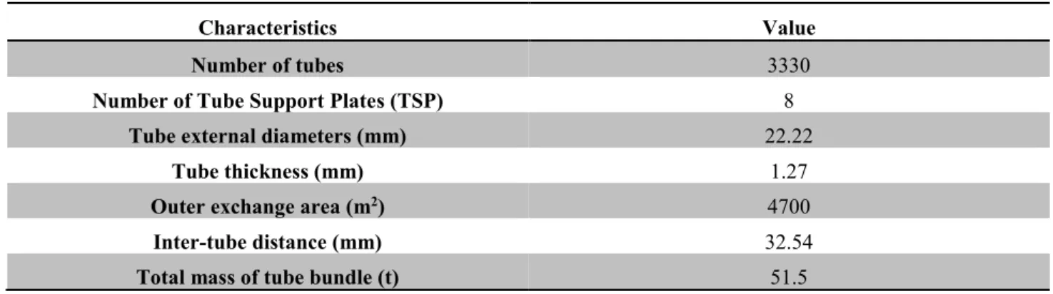
Complete characteristics of the tube bundle of 51B type steam generators are listed in Table 1.1. As the tubes are long and thin, 8 circular plates called Tube Support Plates (TSP) are used for their mechanical maintain (Figure 1.2, left) in 51B type SG. The tubes fit in the circular holes drilled in the TSP. These holes are surrounded by additional quatrefoil holes to let the secondary steam-liquid mixture flow through (Figure 1.2, bottom right). After several decades of operation, deposit formation is observed in the quatrefoil holes between SG tubes and TSP (See TSP clogging phenomenon in Figure 1.2, top right).
Figure 1.2: Scheme of 51B-type PWR recirculating steam generator (Bodineau and Sollier, 2013; Girard et al., 2013). TSP clogging phenomenon is observed after several decades of operation and is represented at the top right.
Table 1.1: Main characteristics of tube bundles used in 51B-type steam generators (Girard, 2014).
Characteristics Value
Number of tubes 3330
Number of Tube Support Plates (TSP) 8
Tube external diameters (mm) 22.22
Tube thickness (mm) 1.27
Outer exchange area (m2) 4700
Inter-tube distance (mm) 32.54
Total mass of tube bundle (t) 51.5
1.2.3
Thermohydraulics in PWR steam generator
TSP clogging phenomena are highly dependent on the thermohydraulics. A general knowledge of PWR SG thermohydraulics is necessary for the further discussions in the present work. In this section, basic notions of two-phase flow parameters, as void fraction, are introduced and defined and different two-flow patterns are presented. Most TSP clogging phenomenon has been observed on the 8th TSP in the EDF NPPs. After describing
fundamentals of two-phase flow typical values of major thermohydraulic parameter on the 8th TSP of 51B type
SG will be identified in section 1.2.3.2 since thermohydraulics will govern TSP clogging phenomena.
1.2.3.1 Two-phase flow fundamentals
Basic theory and definitions are introduced in this section. Given that there are many two-phase flow models in the literature and the objectives of this section is not to give a thorough description of two-phase flow models, only few of them are presented hereafter and the reader can find more information about these models elsewhere in the literature (Cong et al., 2013, 2015; Rummens, 1999; Vergnault et al., 2008; Zohuri and Fathi, 2015).
1.2.3.1.1
Two-phase flow system basic notions
The primary parameters used in two-phase flow modelling are (Royer, 2015): • Thermal: thermal power, temperature, heat flux, etc.
• Hydraulic: pressure, mass flow rate, fluid temperature, pressure drop, etc.
• Geometric: flow and heated areas, hydraulic and heated equivalent diameters, etc.
Along with these primary parameters, in two-phase flow analysis, the following calculated parameters are commonly used:
• Mass flux
• Dynamic mass quality • Void fraction
In addition, two-phase flow calculations require information about fluid properties such as density, viscosity, enthalpy, thermal conductivity, and heat capacity, which depends on the above-mentioned primary fluid parameters. Major basic two-phase flow notions will be briefly defined and presented as following:
Void fraction α (dimensionless) is defined as the volumetric fraction of vapour phase or the cross-sectional area occupied by vapour phase (Av) to the total flow area of a pipe (A) in the limit case of a “thin” volume (Royer,
2015), as expressed in Eq. 1-1. The opposite of void fraction is the liquid fraction.
α = Av
A , (1 − α) = Al
A 1-1
where Al represents the cross-sectional area occupied by liquid phase.
Dynamic mass quality x or steam quality (dimensionless) is defined as the ratio of vapour mass flow Wv (kg/s)
to total mass flow W (Eq. 1-2). The opposite is the liquid quality.
x = Wv
W , (1 − x) = Wl
W 1-2
where Wl represents the liquid mass flow (kg/s).
Mass flux φ is the mass flow rate per unit flow area (Wv/l/A) (kg/s/m2). Vapour and liquid phase fluxes are
defined using steam quality, as in Eq. 1-3.
φv = φx, φl = φ(1 − x) 1-3
The vapour phase velocity vv and the liquid phase velocity vl (m/s) can be expressed in Eq. 1-4 and Eq. 1-5 ,
using the volumetric flow Q(m3/s).
vv = Qv Av = Wv ρvAv 1-4 vl = Ql Al = Wl ρlAl 1-5
Where v and l denote the density of vapour and liquid, respectively.
Using the previous relationships, the ratio between the vapour and liquid velocities in a two-phase flow system, called slip ratio Sv/l (dimensionless), can be expressed as:
𝑆𝑣/𝑙= ( x 1 − x)( ρl ρv )(1 − α α ) 1-6
The vapour in a moving two-phase flow system trends to move at a higher velocity than the liquid because of its buoyancy, density and different resistance characteristics. Experimental data or theoretical correlations for Sv/l covering all possible operating and design variables do not exist. Experimental values of Sv/l under conditions
defined for a particular design are difficult to obtain experimentally. Such procedures are usually expensive and time-consuming. In calculations and modelling, the usual procedure is to neglect the difference between vapour phase and liquid phase velocities or to assume a constant value of Sv/l throughout the fuel channel.
Other parameters, like static quality (vapour mass fraction Cg) or thermodynamic quality of the two phases are
less used because they do not bring relevant information about the flows (velocities). The associated definitions can be found in (Royer, 2015).
1.2.3.1.2
Two-phase flow patterns
Multiphase flow is classified according to the internal phase distributions or "flow patterns" or "regimes". For instance, in the case of a two-phase mixture of a gas or vapour and a liquid flowing together in a channel, different internal flow geometries or structures can occur depending on the size or orientation of the flow channel, the magnitudes of the gas and liquid flow parameters, the relative magnitudes of these flow parameters, and on the fluid properties of the two phases. In particular, two-phase flow patterns are strongly influenced by phase mass flow rates or velocities (K. Popov, 2015). The sequence of flow patterns generally encountered in vertical two-phase flow as a function of the steam quality x is shown in Figure 1.3.
The bubbly pattern means that the vapour phase is distributed in discrete bubbles within a liquid continuum. When the concentration of bubbles becomes higher, bubble coalescence occurs and progressively, the bubble diameter approaches that of the tube. The slug flow (also named plug flow) regime is entered. As the vapour flow is increased with steam quality, the velocity of these bubbles increases and ultimately, a breakdown of these bubbles occurs leading to an unstable regime. In this regime, there is an oscillatory motion of the liquid upwards and downwards in the tube (churn flow). Annular flow represents the pattern where the liquid flows on the wall of the tube as a film and the gas phase flows in the centre. Finally, in the disperse droplet pattern, the liquid phase loses contact with the tube and forms concentrated individual liquid droplets more or less homogenously in the flow.
Figure 1.3: Two-phase flow patterns’ sequence as a function of steam quality x (K. Popov, 2015). “G” and “L” represents the vapour phase and the liquid phase, respectively.
Two-phase flow parameters change significantly from one flow pattern to another one. In particular, the interfacial area between the two phases has a significant impact on the exchange of mass, momentum, and heat between phases. Various two-phase flow parameters are affected differently by flow patterns, and hence various correlations and models are needed to capture phenomena for each flow pattern. This implies the need for well-defined and predictable flow patterns in two-phase flow modelling. Many pattern maps are reported in the literature from experiments or calculations (Cheng et al., 2008). They give a good description of the two-phase flow pattern as a function of flow properties such as steam quality, mass flux, etc. However, most of these pattern maps are limited to relatively low temperature systems (from 20 to 80 °C) and they are not relevant for describing water/vapour flow systems like those reported in PWR SG. More experiments are then required under the same thermohydraulic conditions as those reported in SG. Nevertheless, plot of such map patterns is
particularly challenging because it needs to develop new sensors, which can operate at high temperature and pressure (Hogsett and Ishii, 1997). Efforts are currently made at CEA Cadarache (France) for the development of such two-phase flow measuring sensors (Dupré et al., 2016).
1.2.3.2 Thermohydraulics of 51B type steam generators
Numeric simulations based on porous media models and experimental single-phase and steam-water two-phase flow investigations were performed by several groups (Cong et al., 2013, 2015; Tian et al., 2016; Zhang et al., 2017) to investigate the thermohydraulic characteristics of PWR steam generators. Heat transfer from primary to secondary side, pressure drop for a vertical two-phase flow across a horizontal rod bundle and the effects of power level on thermohydraulic characteristics were discussed. However, only few data are available in the literature about basic parameters in a specific localization in SG like at the 8th TSP of 51B type SG (void fraction,
secondary temperature, etc.).
An EDF modelling tool (THYC) was used for investigating thermohydraulic parameters at the 8th TSP of 51B
type SG (Schindler, 2010, 2016). Schindler’s works summarized the main results of this study and showed the dynamic steam quality varies from about 0.22 to 0.38 on the hot leg side of the 8th TSP. The maximal steam
quality is located at the centre of the tube bundle while a steam quality of 0.30 is observed in the intermediate region between the centre and the wall (see definition of the steam quality x in Eq. 1-2). The void fraction (, Eq. 1-1) reaches 0.85 on the hot leg of 8th TSP with a relatively homogeneous distribution. The pressure is equal
to 61.5 bars in the whole 8th TSP section with a temperature of 277.2 °C in the secondary flow. A mean vertical
velocity of the two-phase flow of about 3 m/s has been calculated at the intermediate region of the hot leg of the 8th TSP. From these calculated thermohydraulic parameters, the two-phase flow located in the 8th TSP is
often supposed to have a disperse droplet regime because of the high void fraction and dynamic steam quality. However, neither experimental nor theoretical works have been performed to confirm such an expectation because of the difficulties mentioned previously.
1.2.4
Materials used in the secondary circuit
In the secondary circuit, the fluid circulation piping is made of carbon steel. SG tube sheet, turbine rotors, high-pressure heater, condensate and feedwater piping are usually made of carbon steel or low alloy steels (Feron, 2012). The steam generator tubes are made of nickel-based alloys: alloys 600 MA (MillAnnealed: thermal treatment at 980 °C for 15 minutes), alloys 600 TT (Thermally Treated at 700 °C for 16 hours) or alloys 690 TT for the most recent steam generators (Le Calvar and De Curières, 2012). The SG Tube Support Plates (TSP) are nowadays made of stainless steel with about 13%wt of chromium (Delaunay, 2010). Condenser tubes are
Most TSP clogging phenomenon is observed on the 8th TSP of PWR 51B type steam generator’s secondary
side. A general description of PWR secondary circuit and steam generators has been done. Important thermohydraulic notions have been introduced and associated parameters have been identified specifically for the 8th TSP region in 51 B type SG in order to feed further discussion in the present work. Thereafter,
the major source term of TSP clogging phenomenon will be identified, by firstly introducing the different materials used in the secondary circuit and the associated corrosion phenomena under the specific PWR secondary water chemistry. Magnetite is the stable form of iron species under PWR SG conditions and is the main composition of TSP clogging. Its structural and physio-chemical properties will be provided.
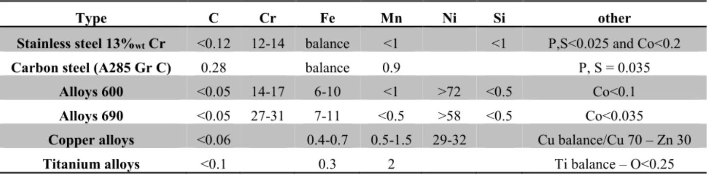
made of stainless steels, or copper alloys or titanium-based alloys. Chemical compositions (%wt) of alloys
usually used in PWR secondary circuit are gathered in Table 1.2.
Table 1.2: Chemical composition (in %wt) of alloys usually used in PWR secondary circuit.
Type C Cr Fe Mn Ni Si other
Stainless steel 13%wt Cr <0.12 12-14 balance <1 <1 P,S<0.025 and Co<0.2
Carbon steel (A285 Gr C) 0.28 balance 0.9 P, S = 0.035
Alloys 600 <0.05 14-17 6-10 <1 >72 <0.5 Co<0.1
Alloys 690 <0.05 27-31 7-11 <0.5 >58 <0.5 Co<0.035
Copper alloys <0.06 0.4-0.7 0.5-1.5 29-32 Cu balance/Cu 70 – Zn 30
Titanium alloys <0.1 0.3 2 Ti balance – O<0.25
1.2.5
PWR secondary flow chemistry
Slightly alkaline solution in the secondary circuit is used to limit corrosion phenomena in the PWR secondary circuit (Nordmann and Fiquet, 1996). For this goal, most of the nuclear operators use volatile alkaline reagent (AVT, All Volatile Treatments). Two main reagents are used: morpholine (C4H9NO) and ammonia (NH4OH).
Other reagents are less frequently used like ethanolamine (C2H7NO). Hydrazine (N2H4) is used for reducing
dissolved oxygen concentration for Stress Corrosion Cracking (SCC) prevention.
Ammonia was largely used thanks to its easy implementation, low cost and its relatively low decomposition. However, its use is limited in the presence of copper alloys in secondary circuit materialsbecause ammonia corrosion leads to the formation copper ions that form stable copper-ammonia complexes (Cu(NO3)62+) when
pH is higher than 9.4 at 25 °C (Yang et al., 2017a), which participate actively in the corrosion of copper material and increase the risk of copper reprecipitation elsewhere in the secondary circuit. Therefore, pH25 °C is fixed at
between 9.1 and 9.3 in the presence of copper alloys in the secondary circuit. The use of hydrazine in the presence of copper alloys is also limited due to its decomposition inducing the formation of ammonia. Its concentration ranges generally from 5 to 10 µg/kg (ppb) (Delaunay, 2010; Nordmann and Fiquet, 1996; Suat and Francis, n.d.). In the absence of copper alloys, pH25 °C is fixed by ammonia or morpholine around 9.6 to 9.7
to prevent corrosion.
In certain cases, hydrazine concentration can be increased up to 50-100 µg/kg in the absence of copper, especially for enhancing SCC prevention. Morpholine allows providing a homogeneous protection all over the steam-water system since its distribution coefficient (concentration in vapour/concentration in liquid phase) is close to 1. However, more and more operators work on the substitution of morpholine by another reactive because the high concentration of morpholine in secondary circuit and its low thermal stability increase the risk of formation of organic compounds by chemical decomposition such as ethenol and ethenamine (Altarawneh and Dlugogorski, 2012). Ethanolamine (ETA) is a good candidate to replace morpholine. This reactive is for instance largely used in US because it can be used at lower molar concentration than morpholine and thermal decomposition is limited (Suat and Francis, n.d.).
Most chemical elements remain in the liquid phase as their distribution coefficients are generally around 10-4.
In order to limit the corrosion phenomena associated with the presence of these pollutants in the liquid phase, periodical purges of secondary water are performed. A purge rate of 1% of the feedwater flow is generally used in France (Suat and Francis, n.d.), which leads to an estimated super-concentration coefficient in SG water of 100 compared to the feedwater.
In restricted zones of SG as in clogged TSP flow holes, primary tubes’ cooling is less efficient due to the reduced secondary water flow, which may induce local overheating, leading to an increase of pollutant concentrations. The super-concentration coefficient in these regions can reach as high as 106 compared to SG water (Nordmann
and Fiquet, 1996). The current pollutant concentration is maintained below 0.01 µg/kg in the feedwater. Therefore, the concentration in the SG water can then be estimated to be around 1 µg/kg (1 ppb) with a super-concentration coefficient of 100 and the pollutant super-concentration can reach between 1 mg/kg (1ppm) and 1 g/kg. The total iron concentration in the feedwater is measured to be around 30 ppb by EDF (De Bouvier, 2015a). No data is available in the literature for estimating iron concentration in SG water or SG restricted regions by taking into account the super-concentration phenomenon in PWR SG.
The French EDF chemical specification of PWR secondary feedwater is summarized in Table 1.3.
Table 1.3: Principal EDF Chemical specification of PWR secondary feedwater.
Parameters Value
pH25 °C 9.1 to 9.3 with copper alloys 9.6 to 9.7 without copper alloys
Hydrazine concentration (ppb) 5 to 10 with copper alloys 50 to 100 without copper alloys
Oxygen concentration (ppb) < 3
Redox potential (V/SHE) -0.4
Total iron concentration (ppb) 30
Impurities (sodium, chlorine…)
concentration(ppb) < 1
1.2.6
Corrosion phenomena in PWR secondary circuit
The PWR secondary water chemistry management, previously presented, aims at protecting the whole secondary circuit towards corrosion phenomena. Flow accelerated corrosion (FAC) of components in carbon steel is found to be the major term source of TSP clogging formation. Effects of different parameters, as material composition and flow thermohydraulics, will be discussed based on previous studies available in the literature. Stress corrosion cracking (SCC) majorly affects SG tubes in alloy 600 and will be briefly presented.
SCC will be firstly introduced, affecting majorly SG tube materials. FAC is believed to be the major source of TSP clogging phenomenon. Effects of major parameters, as pH and oxygen concentration, will be carefully discussed in paragraph 1.2.6.2.
1.2.6.1 Stress corrosion cracking (SCC)
SCC is responsible for material cracking under both environment and mechanical stresses. The propagation rate of SCC ranges generally from 10-5 to 1 µm/s and increases with stress (Arioka et al., 2006).
Steam generator tubes in the secondary circuit constituted of Alloy 600 MA suffered from SCC. Such SCC induced intergranular stress corrosion cracking (IGSCC) and intergranular attack (IGA). A generic designation for these secondary side degradations is IGA/IGSCC because they are often observed together.
SCC of Alloy 600 MA has been carefully discussed from a mechanistic point of view by Delaunay (Delaunay, 2010). A double-layer deposit composed of a compact inner layer enriched in chromium and a porous outer layer containing nickel oxides was observed onto Alloy 600 surface undergoing SCC.
IGA/IGSCC is mostly found in restricted regions as between the tubes and the TSP. In these locations, the flow of secondary fluid is restricted, which may be further impeded by the presence of corrosion product deposits, like TSP clogging, inducing even more restricted geometries. The restricted flow conditions enable a local super-concentration of any impurities, as previously mentioned in paragraph 1.2.5. Severe chemical conditions can thus be obtained, which are capable to induce IGA/IGSCC of Alloy 600 MA tubes. The main detrimental polluting elements are sodium, sulfur, copper and lead (De Bouvier, 2015b; Feron, 2015).
Alloy 600 TT, Alloy 690 TT and stainless steel suffer much less from IGA/IGSCC than Alloy 600 MA. The older carbon steel TSPs with drilled holes have been more subject to IGA/IGSCC since they undergo more easily concentrated crevice environment than those with current stainless steel quatrefoil tube holes.
1.2.6.2 General corrosion and Flow accelerated corrosion (FAC)
According to the International Standard ISO 8044, general corrosion of metallic materials is defined as a “general proceeding at almost the same rate over the whole considered surface” (Féron and Richet, 2010). In an aqueous environment, such as water-cooled reactors like PWR, metallic materials corrosion is of electrochemical nature (Feron, 2015), with the metal oxidation as anodic reaction and the reduction of dissolved oxygen or water as cathodic reaction. General corrosion is characterized by these basic electrochemical reactions that take place uniformly over the whole considered surface. If the corrosion products are soluble, general corrosion is evidenced by a decrease in metal mass or thickness over time; if the corrosion products are not soluble, the corrosion is evidenced by the formation of a uniform layer of corrosion products which may be more or less protective against further corrosion. Iron contained in carbon steel is oxidized into magnetite form under typical PWR SG conditions, predicted by various authors using Pourbaix diagrams (Chexal et al., 1998; Chivot, 2004; Delaunay, 2010; Mansour, 2009; Pourbaix, 1963). Figure 1.4shows that the Pourbaix diagram of iron predicts magnetite as the stable form of iron in deionized and degassed reducing water (Eh = -0.4 V vs. SHE) at 200 °C and pH200 °C > 6 (pH25 °C > 9).
Figure 1.4: Pourbaix diagram of iron calculated with PHREEPLOT, using the Lawrence Livermore National Laboratory (llnl) database (“llnl.dat”, n.d.). Temperature = 200 °C corresponding to the temperature of the secondary circuit before
entering into the SG; pH25 °C > 9 corresponds to pH200 °C > 6 (Yang et al., 2017a); Potential Eh in Volt given vs. the
Standard Hydrogen Electrode (SHE). Red point indicates that the stable form of iron is magnetite under the above-mentioned conditions.