Assessment of type II diabetes mellitus using irregularly sampled measurements with missing data

Assessment of type II diabetes mellitus using

irregularly sampled measurements with missing data

The MIT Faculty has made this article openly available.

Please share

how this access benefits you. Your story matters.

Citation

Barazandegan, Melissa, Fatemeh Ekram, Ezra Kwok, Bhushan

Gopaluni, and Aditya Tulsyan. “Assessment of Type II Diabetes

Mellitus Using Irregularly Sampled Measurements with Missing

Data.” Bioprocess and Biosystems Engineering 38, no. 4 (October

28, 2014): 615–629.

As Published

http://dx.doi.org/10.1007/s00449-014-1301-7

Publisher

Springer Berlin Heidelberg

Version

Author's final manuscript

Citable link

http://hdl.handle.net/1721.1/107276

Terms of Use

Article is made available in accordance with the publisher's

policy and may be subject to US copyright law. Please refer to the

publisher's site for terms of use.

(will be inserted by the editor)

Assessment of type II diabetes mellitus using irregularly sampled

measurements with missing data

Melissa Barazandegan · Fatemeh Ekram · Ezra Kwok · Bhushan Gopaluni · Aditya Tulsyan

the date of receipt and acceptance should be inserted later

Abstract Diabetes Mellitus is one of the leading diseases in the developed world. In order to better regu-late blood glucose in a diabetic patient, improved modelling of insulin-glucose dynamics is a key factor in the treatment of diabetes mellitus. In the current work, the insulin-glucose dynamics in type II diabetes mellitus can be modelled by using a stochastic nonlinear state-space model. Estimating the parameters of such a model is difficult as only a few blood glucose and insulin measurements per day are available in a non-clinical setting. Therefore, developing a predictive model of the blood glucose of a person with type II diabetes mellitus is important when the glucose and insulin concentrations are only available at irregular intervals. To overcome these difficulties, we resort to online Sequential Monte Carlo (SMC) estimation of states and parameters of the state-space model for type II diabetic patients under various levels of randomly missing clinical data. Our results show that this method is efficient in monitoring and estimating the dynamics of the peripheral glucose, insulin and incretins concentration when 10%, 25% and 50% of the simulated clinical data were randomly removed.

Keywords Type II diabetes mellitus·Online identification·Bayesian framework·SIR particle filtering

1 Introduction

Diabetes mellitus is a serious disorder that can cause death [1]. It occurs when the control of blood glucose levels fails. Glucose is produced in the digestive system by consuming food such as bread, potatoes, rice, pasta and fruit. Blood glucose level is regulated by insulin, a hormone secreted from the islet beta cells of the pancreas. Type I and type II diabetes mellitus are two types of diabetic diseases. About ninety percent of people with diabetes are suffering from type II diabetes [1, 2, 3].

Type II diabetes occurs when the pancreas does not produce enough insulin or the human body cells become resistance against insulin [1]. Insulin resistance happens when the sensitivity of peripheral cells to the metabolic action of insulin is decreased due to genetic factors, environmental factors, obesity, hyperten-sion, dyslipidemias, and/or coronary artery diseases [4]. Exercise and healthy dieting can initially control the blood glucose concentration in type II diabetic patients. However, oral anti-diabetic agent and insulin treatment are required in patients with moderate to severe type II diabetes mellitus. Physicians may provide more appropriate treatments if the etiological factors of patients diabetic conditions are known. [5].There-fore, diagnosing or detecting the dysfunction of different organs such as the pancreas, liver, muscles and adipose tissues will be very useful for selecting the suitable medications for diabetic patients.

In diabetic patients, the glucose metabolic rates represent the health status of the liver, muscles and adipose tissues. To measure the glucose metabolic rates in the type II diabetic patients, the measurement M. Barazandegan, F. Ekram, E. Kwok, and B. Gopaluni

Chemical and Biological Engineering Department, University of British Columbia, Vancouver, BC, Canada V6T 1Z3 Tel.: +1 604 827 3192

E-mail: (mbarazandegan)(fekram)(ezra)(bhushan.gopaluni)@chbe.ubc.ca A. Tulsyan

Process Systems and Engineering Laboratory, Department of Chemical Engineering, Massachusetts Institute of Technology, Cambridge MA 02139, United States

of the glucose and insulin concentrations in different parts of the body are needed. However, clinical mea-surements of all necessary concentrations deep inside different organs or tissues are just not practical or realistic. Therefore, physicians mostly rely on a few measurements from patients blood and/or capillary glucose measurements at regular or irregular intervals for clinical decisions [5].

Previous studies have shown that important clinical data may be missing owing to different reasons such as inability to record clinical results, infrequent sampling by patients, and illegible hand writing. Lack of complete knowledge about the health status of the diabetic patients poses more problems to physicians in managing type II diabetes while they need time oriented clinical data of past and present status of diabetic patients [6, 7, 8].

Since only a few blood glucose measurements per day are available in a non-clinical setting, developing a predictive model of the blood glucose of a person with type II diabetes mellitus is important. Such a model may provide useful information to diabetic patients of dangerous metabolic conditions, enable physicians to review past therapy, estimate future blood glucose levels, and provide therapy recommendations. It can also be used in the design of a stabilizing control system for blood glucose regulations [9, 10].

Many studies proposed on-line identification of type I diabetes mellitus using neural network modelling approaches [10, 11, 12, 13]. Trespet al.[10] developed a predictive model of the blood glucose of a person with type I diabetes mellitus with partially missing clinical data by using a combination of a nonlinear recurrent neural network and a linear error model. However, developing a nonlinear state-space model for type II diabetes mellitus that can easily deal with missing data has received limited attention. The compartmental minimal modelling (MINMOD) approach for type II diabetes mellitus [14] has been used widely in many studies. Recently, based on the Sorensen model [15], a detailed nonlinear model has been developed by Vahidi

et al.[16] for the type II diabetic patients. However, none of these approaches considered identification of a type II diabetes model from clinical data, which contain missing data at random intervals.

The goal of this work is to develop a blood glucose predictive model for a type II diabetic patient and the model can be estimated by using patient data collected under normal everyday conditions rather than a well-controlled environment typically done in a clinical facility. Such a model should be able to detect dangerous metabolic states of a patient, and optimize the patient’s therapy.

In this study, we use online Bayesian estimation framework to estimate a stochastic nonlinear model for type II diabetes mellitus using clinical data with missing data at random intervals. We adopt the detailed nonlinear model developed by Vahidi et al.[16, 17] for type II diabetes since the Vahidi model is a much more detailed model comparing with the MINMOD approach. The Vahidi model is able to effectively model individual abnormalities by characterizing distinct compartments as the faulty organs. To artificially create clinical data sets with missing data at random intervals, we then randomly remove 10%, 25% and 50% of the original available data obtained from the Vahidi model. At the end, glucose, insulin, and incretins concentrations, as well as the parameters of different compartments, are estimated from clinical data with missing data at random intervals. These estimates can then be used to measure the glucose metabolic rates in different organs of the type II diabetic patients.

There is an extensive discussion on estimating the states and the parameters of the nonlinear state-space models from partially missing data using mathematical approaches such as Bayesian filters, Particle filters (PFs), Expectation-Maximization (EM) algorithms, Sequential Importance Resampling (SIR) particle filters [18, 19, 20, 21]. In many studies, Baysian estimation has been used in metabolism and physiological modelling [22, 23, 24]. Among these methods, we use the SIR based PF proposed by Tulsyan et al. [25] for online Bayesian estimation of the states and the parameters of the Vahidi model since it needs less computational cost when a large number of unknown states and parameters must be estimated simultaneously. To do this, a clinical data set, as well as a prior information on the unknown states and parameters of the Vahidi model, are needed. This kind of information can be gathered from physical considerations and population studies. This paper is organized as follows. In section 2, the mathematical model of type II diabetes mellitus is provided. In sections 3 and 4, a summary description of the SIR filtering algorithm is discussed. The on-line parameters estimation results of the nonlinear type II diabetic model are presented in section 5 when 10%, 25% and 50% of missing clinical data are removed randomly. Then, the application of SIR particle filter-ing technique in detectfilter-ing the organ dysfunction of a group of type II diabetic patients under irregularly sampled clinical data is presented.

2 Mathematical modelling of the type II diabetes mellitus

The model of the glucose-insulin interaction in type II diabetic patients used here is based on the Vahidi model [16]. In this model, the concentrations of three substances (i.e., glucose, insulin and glucagon) and

their interactions are described by three main models based on the Sorensen model [15]. Each sub-model is divided into individual numbers of compartments representing specific parts or organs of a human body. The number of compartments is different in each sub-model. As can be seen in Fig. 1, the insulin sub-model has seven compartments: brain, liver, heart and lungs, periphery, gut, kidney, and pancreas. The blocks represent different compartments and the arrows indicate the blood flow directions. The glucose sub-model is similar to the insulin sub-model except that the pancreas compartment is excluded. Since the glucagon concentration is considered to be identical in all parts of the body, only one compartment is used in the glucagon sub-model [26]. In each sub-model, mass balance equations are written for all individual sub-compartments (except for the pancreas, which will be described in more details in Appendix A). The general form of the mass balance equation on each sub-compartment is shown as follows [27]:

VdY

dt =Q(Yin− Yout) +rp− rc. (2.0.1)

whereV is the volume of sub-compartments,Y is the concentration of either insulin, glucose, or glucagon,t

is time,Qis blood flow rate, andrP andrCare metabolic production and consumption rates of the material balance substance, respectively. Since the glucagon sub-model has only one compartment, blood flow rate is set to zero and the glucagon mass balance equation has only the metabolic production and consumption rates. The metabolic rate of different substances takes on the following general form [27]:

r=MI(t, I)MG(G)MΓ(t, Γ)rB. (2.0.2)

whereI,G, andΓ represent insulin, glucose, and glucagon substances, respectively.Miis thei’s multiplier, which represents the regulatory effect ofisubstance on the metabolic rate, andrB is the metabolic rate at the basal condition. The general mathematical form of multiplicative effect of each substance is [27]:

Mi=A+Btanh[C( i

iB − D)]. (2.0.3)

whereiBis the concentration ofiat basal condition andA,B,C, andDare parameters, which are unknown and should be estimated.

Later, the Vahidi model was modified to determine the variations of blood glucose concentration resulted from an oral glucose intake by adding a model of gut glucose absorption in the gastrointestinal tract proposed by Dalla Man et al. [28, 17]. In addition, the hormonal effects of incretins on boosting pancreatic insulin secretion was included by adding a two compartment model of incretins production in order to simulate the variations of incretins concentrations in blood circulatory system. Appendix Acontains the details on the complete model equations.

In the Vahidi model, two different clinical tests, oral glucose tolerance test (OGTT) and isoglycemic intravenous glucose infusion test (IIVGIT) performed by Knop et al. [29, 30], were used for states and parameters estimation. The clinical data sets are summarized in detail in section 5.1. Estimation of the modified model parameters were carried out by minimizing the deviation of model predictions from the available measurements of peripheral glucose, insulin and incretins concentrations. The deviation of model predictions from the measured clinical data is minimized through the following objective function:

min Θ n X j=1 [(Gj−Gˆj)2+ (Ij−Iˆj)2]. (2.0.4)

where Gj and Ij are peripheral glucose and insulin concentrations at time j obtained from the model respectively; ˆGjand ˆIj are the corresponding clinical measurements;nis the number of samples in the clin-ical data set; andΘis the vector of parameters containing the glucose, insulin, and glucagon metabolic rates [16]. Different parameters of metabolic rates will be obtained after the optimization procedure for each type II diabetic patient since there are different peripheral glucose, insulin and incretins concentrations profile for different patients.

In this study, the estimation of the Vahidi model parameters are carried out by the SIR particle filtering method for data sets that contain randomly deleted simulated data described in the following sections. To do this, the continuous time stochastic nonlinear state-space format of the Vahidi model [17] in equation (2.0.1) is transformed to discrete time format as follows:

b

yt=g(xbt,θbt, ut), (2.0.5)

wheregis the measurement dynamic function variables andybtis the vector of concentration of either insulin, glucose, or glucagon at sampling timet(Y in equation (2.0.1)) monitored and recorded by several sensors and measuring devices. These devices record patient’s critical variablesyt(output) in response to the test actionut(input) implemented at some point in time indexed byt. For example, in the intravenous glucose infusion test, insulin concentration measurements as output yt are recorded at regular intervals against the infused glucose concentration as inputut. A summary description of this on-line estimation method is provided in the next following sections.

3 Response models

In clinical trials, several sensors and measuring devices were used for monitoring the response of a pa-tient to a clinical test. Let us assume that we have a sequence of time-tagged clinical measurements

y1:t={y1, y2, . . . , yt} corresponding to the input action u1:t={u1, u2, . . . , ut}, and that we are interested in predicting the response yt+1 for some known input action ut+1. Such predictions are valuable to the physician assessing the health of the patient during clinical trials. To solve this problem, we can assume

yt+1 is independent of{u1:t, y1:t}, in which case, the prediction ofyt+1 is impossible. Alternatively, we can assumeyt+1 depends on the trend recorded in the past data{u1:t, y1:t}. For the latter assumption– which is true for any causal system– a response model1is useful in predicting the response of a patient to a clinical test.

A reliable response model should not only accurately model a patient’s physical and biological response to a clinical test, it should also account for the various uncertainties such as modelling and measurement errors. For example, random measurement errors can be modelled by viewingyt as a random realization of a stochastic process. In this work, we use stochastic state-space models (SSMs) to represent a response model. Mathematically, a SSM can be represented as:

xt+1=f(yt, θt, ut) +vt, (3.0.6a)

yt=g(xt, θt, ut) +wt, (3.0.6b)

1 _{A response model is a mathematical model describing the dynamics of the key internal states of a patient in response}

wherextdescribes evolution of the internal states of the patient. Physically,xtmodels the complete response of a patient subject to a clinical test. Given the statesxt, inputsutand model parametersθtat timet, the internal states evolve toxt+1.vtin equation(3.0.6a) is the state noise, which accounts for the unknown and unmeasured variations in the states not captured by the response model. Due to the non-zero random state noisevt, the states are not precisely known. Equation (3.0.6b) describes how sensor readings yt relate to the statesxtand parameters θt.wt in equation (3.0.6b) is the noise term, which accounts for the random sensor noise. In clinical trials, measurements of only a few critical states are available at our disposal. This is because the high cost or lack of appropriate sensing technology or devices precludes measurement of all but key internal states. The state-space modelling framework is general, and can be used to represent a wide class of response models, including the type II diabetes mellitus response model given in section 2.

In this paper, we use equation (3.0.6) for real-time estimation of the critical response variables, such as blood glucose, insulin and incretins concentrations during clinical trial of patients with type II diabetes mellitus. Monitoring these variables is critical as it enables the physicians to review past therapy, estimate future blood glucose levels and provide therapy recommendations. To predict the critical variables using equation (3.0.6), the model states and parameters, which are typically unknown for a patient need to be estimated first. Given the state and parameter estimates, the model predictions attcan be computed as:

b

yt=g(bxt,θbt, ut), (3.0.7)

where y_bt is the response predictions and xbt and bθt are the parameter and state estimates, respectively. Ideally, given an accurate estimate of the states and parameters, the model predictions should match the clinical measurements as closely as possible. Any standard estimation approach involves fitting the model using available clinical measurements; however, data fitting is not straightforward for SSMs because of the following reasons: 1) the states are stochastic, which makes estimation of both states and parameters challenging and 2) the clinical measurements are assumed to be irregularly sampled.

In this paper, we propose the use of Bayesian methods for real-time state and parameter estimation in equation (3.0.6) under irregularly sampled clinical measurements. In the next section, a description of real-time Bayesian estimation is provided.

Remark.There is a much larger appeal to use state-space modelling framework to represent response models. From equation (3.0.7), it is evident that computing the response predictions using a SSM also requires estimation of all the internal states of the patient. Thus, any method designed to compute the response predictions gives away estimation of all the internal states as a side product. This is of immense value to a physician, considering only a handful of the internal states are actually measured.

4 Real-time Bayesian estimation

Our objective is to estimate zt in real-time using clinical data {u1:t;y1:t}. Let zt = {xt, θt} denote an extended vector of unknown states and parameters. It is further assumed that the clinical measurements are recorded at irregular times, such that only a subset ofy1:tis available for estimation att. For notational convenience we dispense with the inpututin the succeeding discussions; however, the method presented in this paper holds with the inputs included.

In the Bayesian framework, the variables to be estimated are assumed to be random variables. The states are inherently random due to the noise in equation (3.0.6a); and the parameters, which are unknown but non-random are assumed to be random, such thatzt={xt, θt}is a vector of random variables. To set up the Bayesian estimation, we assumez0to be distributed with a prior densityp(z0|y1:0). Also, we assume the state and measurement noise are independent and identically distributed (i.i.d) zero mean finite variance Gaussian sequences with the probability density functions (PDF)px(.) andpy(.) knowna priori.

4.1 Complete clinical data

First we consider the estimation problem using the complete clinical data set. Assumingy1:tto be available, the real-time Bayesian estimation ofztattinvolves computing the posterior densityp(zt|y1:t). Here,p(zt|y1:t) is a probabilistic representation of the statistical information available on zt conditioned on the clinical measurements y1:t. Using the Bayes’ theorem and Total law of probability, p(zt|y1:t) can be recursively computed in two steps, which are the update and prediction steps as shown below:

Update Step:

Prediction Step:

p(zt|y1:t−1) = ˆ

pz(zt|zt−1)p(zt−1|y1:t−1)dzt. (4.1.2)

In equation (4.1.1),py(yt|zt) is the measurement noise distribution or the likelihood function indicating how likely it is for zt to have generated the clinical measurementyt.p(zt|y1:t−1) is a one-step-ahead prior density representing statistical information onztprior to the recorded clinical measurement yt. The prior density p(zt|y1:t−1) is computed using equation (4.1.2), wherepz(zt|zt−1) is the joint state and parameter noise distribution andp(zt−1|y1:t−1) is the posterior distribution att −1.

Starting with p(z0|y0:1), in principle, the recurrence relation between equations (4.1.1) and (4.1.2) pro-vides a complete Bayesian solution to the state and parameter estimation problem under complete clinical data. Finally usingp(zt|y1:t), the estimate ofzbtattcan be computed as the mean of the posterior density, such that the estimate step can be defined as:

b

zt= ˆ

ztp(zt|y1:t)dzt, (4.1.3)

wherezbt={bxt,θbt}is the state and parameter estimation att. Note that other values, such as the mode or median ofp(zt|y1:t) can also be selected as the point estimate.

4.2 Irregular clinical data

From section 4.1, it is evident that if yt is not measured at t, the posterior density p(zt|y1:t) cannot be computed using equation (4.1.1). In such situations, the estimates att, in presence of irregular data can be computed by replacingp(zt|y1:t) in equation (4.1.3) using the one-step ahead prior densityp(zt|y1:t−1).

Now assumingyt+1 to be available att+ 1, the posterior density forzt+1, given clinical measurements

{y1:t−1, yt},i.e.,p(zt+1|y1:t−1, yt+1) can be computed using the Bayes’ theorem and the law of total proba-bility, such that the update step shows that:

p(zt+1|y1:t−1, yt+1)∝ p(yt+1|zt+1)p(zt+1|y1:t−1). (4.2.1)

wherep(zt+1|y1:t−1, yt+1) is the posterior density forzt+1andp(zt+1|y1:t−1) is a two-step ahead prior density computed using the law of total probability,i.e.:

p(zt+1|y1:t−1) = ˆ

pz(zt+1|zt)p(zt|y1:t−1)dzt. (4.2.2)

Substituting equation (4.1.2) into equation (4.2.2) yields the prediction step:

p(zt+1|y1:t−1) = ¨

pz(zt+1|zt)pz(zt|zt−1)p(zt−1|y1:t−1)dzt−1:t. (4.2.3)

Similar to section 4.1, having computed p(zt+1|y1:t−1, yt+1), the estimate of zt+1 can be computed by replacing the density by p(zt+1|y1:t−1, yt+1) in equation (4.1.3). Note that the method proposed in this section is general and can naturally be extended to handle consecutively missing measurements as well.

The Bayesian approach developed in section 4 provides an excellent framework for real-time state and parameter estimation under complete and irregular clinical measurements. Computing the Bayesian solution requires evaluation of the multiple integrals in the prediction and estimation steps. Unfortunately, except for linear systems with Gaussian state and measurement noise, or when the states and parameters take on only finite values, the Bayesian solution cannot be solved exactly with finite computing capabilities.

This paper uses a sequential Monte-Carlo (SMC)-based adaptive sequential-importance-resampling (SIR) filter proposed by Tulsyanet al.[25] to numerically approximate the Bayesian solution. In the next section, using SMC method, the estimation results of states and parameters of the state-space model for type II diabetic patients under various levels of randomly missing clinical data are presented.

5 Results and discussion

In this section, the efficiency of the SIR filtering method in handling missing measurements for estimation of the nonlinear stochastic model for type II diabetes mellitus is demonstrated. All the simulations were conducted on a 2.90 GHz CPU with 8 GB RAM Mac using MATLAB 2012b. On-line estimation of states and all the parameters cited in the reference [17] by SIR filtering leads to large memory requirements and computational complexity. To reduce the computation load, only the parameters of type II diabetic subjects that have considerable effects on peripheral glucose, insulin and incretins concentrations were chosen for estimation while keeping all other non-essential model parameters constant.

5.1 Clinical data used for model development

The states and the parameters of the Vahidi model were estimated using two different clinical tests, oral glucose tolerance test (OGTT) and isoglycemic intravenous glucose infusion test (IIVGIT) performed by Knop et al. [29, 30]. In the OGTT test, glucose was given to the patient subjects and their blood was sampled afterward to determine how quickly glucagon suppression occurred.

In the OGTT test, 50-grams of water-free glucose was dissolved in 400 millilitres of water over the first 5 minutes of the experiment. The solution was given to 10 patients with type II diabetes mellitus (eight men and two women). Blood was sampled 15, 10 and 0 minutes before, and after the ingestion of glucose at 5, 10, 15, 20, 30, 40, 45, 50, 60, 70, 90, 120, 150, 180 and 240 minutes.

In order to mimic the plasma glucose profile obtained from the OGTT test, the same amount of glucose was injected intravenously to the diabetic subjects in the IIVGIT test. Blood was sampled every 5 minutes [29, 30]. For estimating the states and the parameters of the model in our study, the peripheral glucose, insulin and incretins (GLP-1 plus GIP) concentrations from both tests were used.

5.2 On-line states and parameters estimation results

To apply the SIR particle filtering method, a prior information on the unknown parameters of the Vahidi model from both OGTT and IIVGIT is needed. This information can be obtained from equation (2.0.4) by minimizing the deviation of model predictions from the available clinical measurements of peripheral glucose, insulin and incretins concentrations described in section 5.1.

After the prior information on the unknown parameters obtained, the estimation of the states and param-eters of the Vahidi model were estimated using SIR particle filtering method. Firstly, the paramparam-eters of the pancreas model were estimated from the isoglycemic intravenous glucose infusion test (IIVGIT) test since no secretion of incretins occurs during the IIVGIT test. In the model parameter estimation, the peripheral insulin concentration in the Vahidi model [17] was considered as a measurementyk. For implementing the SIR filtering based on the discrepancies between the Vahidi model and the Knop’s experimental data, the following parameters were selected:

• The number of particlesN = 5000

• The sampling time used for discretizing the Vahidi model∆k= 0.4min • The maximum states noisesvk∼ N(0,0.001)

• The measurement noisewk ∼ N(0,0.001)

A priori information on{x0;θ}includes the lower (LB) and the upper bound (UB) based on the phys-iological considerations. Four simulation experiments were carried out to evaluate the effectiveness of our proposed method to identify patient models with incomplete data. In the four experiments, 0%, 10%, 25% and 50% of available data simulated from the Vahidi model were removed randomly. For example, when 10% of data were considered missing, a peripheral insulin concentration at each sampling time was removed from the original data set if a uniformly distributed random variableq in the interval (0,1) is less than 0.1. Similar experiments were done with 25% and 50% missing data [20].

The parameter values after 600 samples from each of these experiments are shown in Table 1. The detailed information about these parameters is available by Vahidiet al.[17]. For all the experiments, the parameters converged to the neighbourhood of the original values after a certain number of iterations.

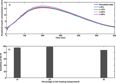
Variations of the peripheral insulin concentrations during the IIVGIT test after 600 samples are shown in Fig. 2a in which,rshows the percentage of missed observations. From the Fig. 2a, the dynamics of peripheral insulin concentration can be estimated reasonably well with physiological responses in all the experiments even when 50% of the simulated clinical data were absent. Fig. 2b presents the goodness of fit between the

Table 1: Parameter estimation results for insulin sub-model after 600 sampling time during IIVGIT test

Parameters [17] OriginalValues Percentage of Missing insulin measurements

0% 10% 25% 50% θ1:α(min)−1 0.6152 0.6168 0.5728 0.5803 0.5159 θ2:γ(U/min) 2.3665 2.3422 2.1860 2.3667 2.5200 θ3:K(min)−1 0.0572 0.0565 0.0560 0.0561 0.0544 θ4:N1(min)−1 0.0499 0.0496 0.0519 0.0481 0.0474 θ5:N2(min)−1 0.0001490 0.0001489 0.0001482 0.0001500 0.0001506

estimated output and the measured output performed with MATLAB System Identification Toolbox by using normalized root mean square error (NRMSE) as a cost function. Based on the NRMSE measure, the goodness of fit between the simulated peripheral insulin concentration and the available measurements are more than 80%. 0 100 200 300 400 500 600 4 6 8 10 12 14 Time (min)

Peripheral insulin concentration (mU/l)

Simulated data r=0% r=10% r=25% r=50% 10 25 50 0 20 40 60 80 100

Percentage of the missing measurments

Goodness of the fit

a)

b)

Fig. 2: Peripheral insulin concentration for type II diabetic subjects during the IIVGIT test

Secondly, from the oral glucose tolerance test (OGTT), the peripheral insulin concentration, peripheral glucose concentration and incretins concentrations were considered as measurementsykfor estimation of the rest of the model parameters. These parameters consist of the parameters of the incretins sub-model and those of the glucose sub-model including the parameters of the glucose absorption model and the parameters describing the hormonal effects of incretins on the pancreatic insulin production. For implementing the SIR filtering based on the discrepancies between the Vahidi model and the Knop’s experimental data, the following parameters were selected:

• The number of particles N= 20000

• The maximum states noisesvk∼ N(0,0.7)

• The measurement noisewk ∼ N(0,0.7)

The parameter values after 2400 samples from each of these experiments are shown in Table 2 (see the reference [17] for detailed information about these parameters). In all the experiments, the estimated parameters, exceptθ3andθ10, converged to the neighbourhood of the original values after a certain number of iterations.θ3 andθ10 are not estimated precisely since the sensitivity of the KLD in kernel smoothing algorithm to changes inθ3 andθ10, is smaller than its variance.

Table 2: Parameter estimation results for insulin sub-model after 2400 sampling time during OGTT test

Parameters [17] OriginalValues Percentage of Missing insulin measurements

0% 10% 25% 50% θ1:cIP GU 0.0970 0.0965 0.0965 0.0902 0.1300 θ2:cI∞HGU 3.2606 3.3125 2.9543 2.9625 2.8057 θ3:cGHGP 1.0385 1.0352 1.0885 1.9743 2.0649 θ4:cGHGU 2.03 1.97 1.84 2.23 1.53 θ5:dIP GU 2.752 2.747 2.724 2.897 2.909 θ6:dI∞HGU 0.0031 0.0030 0.0028 0.0030 0.0038 θ7:dI∞HGP 0.3648 0.3676 0.3610 0.3625 0.3667 θ8:K12(min)−1 0.0783 0.0796 0.0798 0.0842 0.0616 θ9:ξ1(min)−1 0.000124 0.000125 0.000126 0.000125 0.000141 θ10:ξ2(min)−1 0.00270 0.00271 0.00280 0.00152 0.00122

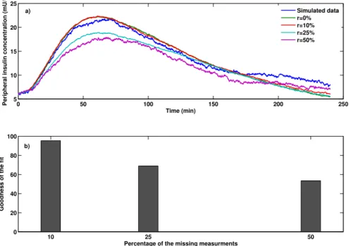
Variations of the peripheral glucose, insulin, and incretins concentrations during the OGTT test after 2400 iterations are shown in Figs. 3a-5a.r shows the percentage of missing observations. From the Figs. 3a-5a, the dynamics of peripheral glucose, insulin, and incretins concentration can be estimated reasonably well with physiological responses in all the experiments even when 50% of the clinical data is missing. Figs. 3b-5b present the goodness of fit between the estimated output and the measured output performed with MATLAB System Identification Toolbox by using the normalized root mean square error (NRMSE) as a cost function. From Figs. 3b-5b, the goodness of fit between the simulated peripheral glucose, insulin and incretins concentration and their available measurements were almost 80% in all the experiments except in Fig. 5b when 25% and 50% of peripheral insulin measurements removed randomly. Comparing to Fig. 2b in the IIVGIT test , the peripheral insulin concentration was not estimated precisely in the OGTT test since only the parameters of the incretins sub-model and the parameters of the glucose sub-model were estimated in order to reduce the computational complexity.

The probability density function of the parameterCIP GU, one of the parameters of the peripheral glucose uptake rate in the insulin sub-model in [27], is reported in Fig. 6. As somewhat expected, the posterior provided by SIR filtering method is concentrated around its original value after about 620 sampling times.

5.3 Application of SIR particle filtering in detection of organ dysfunction in diabetic patients under irregular clinical data

In this section, we will show the application of the adaptive sequential-importance-resampling (SIR) filter in the estimation of the glucose, insulin, and incretins concentrations in different parts of the body under

0 50 100 150 200 250 100 150 200 250 300 350 Time (min)

Peripheral glucose concentration (mg/dl)

Simulated data r=0% r=10% r=25% r=50% 10 25 50 0 20 40 60 80 100

Percentage of the missing measurments

Goodness of the fit

a)

b)

Fig. 3: Peripheral glucose concentration for type II diabetic subjects during the OGTT test

0 50 100 150 200 250 5 10 15 20 25 Time (min)

Peripheral insulin concentration (mU/l)

Simulated data r=0% r=10% r=25% r=50% 10 25 50 0 20 40 60 80 100

Percentage of the missing measurments

Goodness of the fit

a)

b)

Fig. 4: Peripheral insulin concentration for type II diabetic subjects during the OGTT test

irregularly sampled clinical data. These estimates are used for calculating the glucose metabolic rates in different organs of the type II diabetic patients using irregularly sampled data. Then, by comparing the glucose metabolic rate of each organ in the diabetic patients with the glucose metabolic rate of the same organ in a normal subject, the abnormal functioning of certain organs is detected and identified.

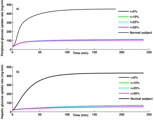
Using the states and parameters of the Vahidi model estimated in the previous section, the glucose metabolic rates in the peripheral tissues and the liver are calculated from equations (2.0.2) and (2.0.3). Figure 7 shows the glucose metabolic rates in peripheral tissues and the liver compared with the healthy subjects. According to Figs. 7a and 7b, the peripheral glucose uptake rate and hepatic glucose uptake rate

0 50 100 150 200 250 −20 0 20 40 60 80 100 Time (min)

Incretins concentration (pmol/l)

Simulated data r=0% r=10% r=25% r=50% 10 25 50 0 20 40 60 80 100

Percentage of the missing measurments

Goodness of the fit

a)

b)

Fig. 5: Incretins concentration for type II diabetic subjects during the OGTT test

0 500 0 500 0 1000 2000 0.0950 0.096 0.097 0.098 0.099 0.1 0.101 1000 2000

Probability density function

CI PGU Iteration #607 Iteration #620 Iteration #600 Iteration #1 d) c) b) a)

Fig. 6: The probability density function ofcI_{P GU} from Bayesian identification at sampling time number 1, 600, 607 and 620 (area under each curve is unitary). They-axis quantity is unit-less.

in type II diabetic patients for all experiments are less than the corresponding values in the healthy sub-jects due to insulin sensitivity in peripheral tissues and dysfunction in the liver of the diabetic patients. Decreased rate of glucose infusion shows that the overall insulin sensitivity of the body is decreased about 54% in diabetic patients. Even under the presence of 50% missing data, the abnormalities of the liver and adipose tissues are detectable, which provides more physiological information to physicians.

0 50 100 150 200 250 0 100 200 300 400 500 Time (min)

Peripheral glucose uptake rate (mg/min)

0 50 100 150 200 250 0 100 200 300 400 500 Time (min)

Hepatic glucose uptake rate (mg/min)

r=0% r=10% r=25% r=50% Normal subject r=0% r=10% r=25% r=50% Normal subject a) b)

Fig. 7: Variation of different glucose metabolic rates

5.4 Strengths and limitations of the SIR particle filtering in clinical practice

The primary practical advantage of the SIR particle filtering method comparing to the traditional statistical methods is its independence from the degree of nonlinearity of the model unlike extended Kalman filtering [5]. An additional advantage in a clinical practice is that the SIR filtering approach is readily adaptable to sequential updating of information obtained from owner history, clinical examination of diabetic patients, and results of different diagnostic tests [31].It exhibits good performance even for systems with large process or measurement noise.

Furthermore, the accuracy of the particle filtering method can be improved by increasing the number of particles used in the estimation algorithm. However, particles size over 1000 can be computationally intensive and time consuming [20, 31]. The SIR based PF used in this paper, needs less computational cost when a large number of unknown states and parameters must be estimated simultaneously since the marginal probability distribution of each parameter and state can be obtained from a posteriori probability distribution of the model parameters and states [24].

6 Conclusions

In this study, we have identified the nonlinear states and the parameters of glucose, insulin and incretins sub-model developed by Vahidi et.al [17] for type II diabetes mellitus in the presence of 10%, 25% and 50% of randomly missing clinical observations by employing the Sequential Importance Resampling (SIR) filtering method. The motivation for this study originates from the lack of complete knowledge about the health status of the diabetic patients. In addition, only a few blood glucose measurements per day are

available in a non-clinical setting due to different reasons like unreadable hand writing, inability to record clinical results, and infrequent sampling by patients.

It is shown that by implementing an on-line SIR particle filtering method to the Vahidi model developed for type II diabetes mellitus, we are able to estimate the dynamics of the plasma glucose, insulin and incretins concentration under the presence of maximum 50% available clinical data. In addition, the goodness of fit between the simulated peripheral glucose, insulin and incretins concentration and their available measure-ments were almost 80% in the most of the experimeasure-ments. The results of this study can be used to inform type II diabetic patients of their medical conditions, enable physicians to review past therapy, estimate future blood glucose levels, provide therapeutic recommendations and even design a stabilizing control system for blood glucose regulation.

Nomenclature

Model variables in the glucose sub-model

G Glucose concentration (mg/dl)

M Multiplier of metabolic rates (dimensionless)

Q Vascular blood flow rate (dl/min)

r Metabolic production or consumption rate (mg/min)

T Transcapillary diffusion time constant (min)

t ime (min)

V Volume (dl)

Model variables in the insulin sub-model

I Insulin concentration (mU/l)

M Multiplier of metabolic rates (dimensionless)

m Labile insulin mass (U)

P Potentiator (dimensionless)

Q Vascular blood flow rate (dl/min)

R Inhibitor (dimensionless)

r Metabolic production or consumption rate (mU/min)

S Insulin secretion rate (U/min)

T Transcapillary diffusion time constant (min)

t time (min)

V Volume (dl)

X Glucose-enhanced excitation factor (dimensionless)

Y Intermediate variable (dimensionless)

Model variables in the glucagon sub-model

Γ Normalized glucagon concentration (dimensionless)

M Multiplier of metabolic rates (dimensionless)

r Metabolic production or consumption rate (dl/min)

t time (min)

V Volume (dl)

Model variables in the incretins sub-model

Ψ Incretins concentration (pmol/l)

r Metabolic production or consumption rate (pmol/min)

t time (min) V Volume (dl) First superscript Γ Glucagon B Basal condition G Glucose I Insulin M ncretins

Second superscript

∞ Final steady state value

Metabolic rate subscripts

BGU Brain glucose uptake

GGU Gut glucose uptake

HGP Hepatic glucose production

HGU Hepatic glucose uptake

IΨ R Intestinal incretins release

KGE Kidney glucose excretion

KIC Kidney insulin clearance

LIC Liver insulin clearance

M Γ C Metabolic glucagon clearance

P Γ C Plasma glucagon clearance

P Γ R Pancreatic glucagon release

P Ψ C Plasma incretins clearance

P GU Peripheral glucose uptake

P IC Peripheral insulin clearance

P IR Pancreatic insulin release

RBCU Red blood cell glucose uptake

First superscripts

∞ Final steady state value

A Hepatic artery B Brain G Gut L Liver P Periphery S Stomach

Second subscripts (if required)

C Capillary space

F Interstitial fluid space

l Liquid

s Solid

Appendix A

Glucose sub-model

The mass balance equation over each compartment in the glucose sub-model results in following equations:

VGBC dGBC dt =Q G B(GH− GBC)− VG_BF TG B (GBC− GBF), (A-1) VGBF dGBF dt = VG_BF TG_B (GBC− GBF)− rBGU, (A-2) VGH dGH dt =Q G BGBC+QGLGL+QGKGK+QGPGP C+QGHGH− rBCU, (A-3) VGG dGG dt =Q G

G(GH− GG)− rGGU+Ra, (A-4)

VGL dGL dt =Q G AGH+QGGGG− QGLGL+rHGP− rHGU, (A-5) VGK dGK dt =Q G K(GH− GK)− rKGE, (A-6) VGP C dGP C dt =Q G P(GH− GP C)− VG_{P F} TG P (GP C− GP F), (A-7)

VGP F dGP F dt = VGP F TG P (GP C− GP F)− rP GU, (A-8)

A detailed description about the metabolic rates is available in [15]. The general form of the metabolic production and consumption rates in each organ is as follows:

r=MIMGMΓMB, (A-9)

and multipliers have the following general form:

MC=a+btanh( C

CB − d), (A-10)

The glucose absorption model that calculates the glucose appearance rate into the blood stream follow-ing an oral glucose intake is considered in the gut compartment of the glucose sub-model as follows:

dqSs

dt =−k12qSs+δ(t), (A-11)

dqSI

dt =−kemptqSs+k12qSI, (A-12)

dqint

dt =−kabsqint+kemptqSI, (A-13)

kempt=kmin+

kmax− kmin

2 {tanh[ϕ1(qSs+qSI− x1D)]−tanh[ϕ2(qSs+qSI− x2D)]}+ 2, (A-14)

ϕ1= 5 2D(1− x1) , (A-15) ϕ2= 5 2Dx2 , (A-16)

Ra=f kabsqint, (A-17)

Incretins sub-model

The incretins production is calculated from the following differential equation:

dψ

dt =ςkemptqS2− rIΨ P, (A-18)

rIΨ P =f

ψ

τ ψ, (A-19)

The mass balance equation over the incretins compartment results in:

dψ

dt =ςkemptqS2− rIΨ P, (A-20)

Insulin sub-model

The mass balance equation over the compartments in the insulin sub-model results in following equations:

VIB dIB dt =Q I B(IH− IB), (A-22) VIH dIH dt =Q I BIB+QILIL+QIKIK+QIPIP V − QIHIH, (A-23) VIG dIG dt =Q I G(IH− IG), (A-24) VIL dIL dt =Q I AIH+QIGIG− QILIL+rP IR− rLIC, (A-25) VIK dIK dt =Q I K(IH− IK)− rKIC, (A-26) VIP C dIP C dt =Q I P(IH− IP C)− VIP F TI P (IP C− IP F), (A-27) VIP F dIP F dt = VI_{P F} TI P (IP C− IP F)− rP IC, (A-28)

The pancreas model contains two compartments. The pancreas model equations include mass balance equations over compartments and correlations between variables. The mass balance equation over each compartment results in:

dm dt =K 0 mSKm+γP − S, (A-29) dmS dt =Km − K 0 mS− γP, (A-30)

The steady state mass balance equation around the storage compartment is:

K0mS =Km0, (A-31)

wherem0 is the labile insulin quantity at a glucose concentration of zero. The rest of the equations for the pancreas model are:

dP dt =α(P∞− P), (A-32) dR dt =β(X − R), (A-33) S= [N1Y +N2(X − R) +ξ1ψ]m x > R, S= [N1Y +ξ1ψ]m x ≤ R, (A-34) P∞=Y =X1.11+ξ2ψ, (A-35) X= G 3.27 H 1323.27+ 5.93G3.02 H (A-36) Glucagon sub-model

The glucagon sub-model has one mass balance equation over the whole body as follows:

VΓdΓ

dt =rP Γ R− rP Γ C, (A-37)

References

[1] Canadian Diabetes Association. “Diabetes facts”. In: (2009).

[2] LC Groop, E Widen, and E Ferrannini. “Insulin resistance and insulin deficiency in the pathogenesis of Type 2 (non-insulin-dependent) diabetes mellitus: errors of metabolism or of methods”. In:Diabetologia

1 (1993).

[3] A Basu et al. “Effects of type 2 diabetes on the ability of insulin and glucose to regulate splanchnic and muscle glucose metabolism: evidence for a defect in hepatic glucokinase activity.” In: Diabetes

49.2 (2000).

[4] R a DeFronzo. “Lilly lecture 1987. The triumvirate: beta-cell, muscle, liver. A collusion responsible for NIDDM.” In:Diabetes 37.6 (1988).

[5] O Vahidi, RB Gopaluni, and KE Kwok. “Detection of organ dysfunction in type II diabetic patients”. In:American Control Conference (ACC) 3 (2011).

[6] Akash Rajak and Kanak Saxena. “Achieving realistic and interactive clinical simulation using case based TheraSim’s therapy engine dynamically”. In:Proceedings of the National Conference . . . (2010). [7] CM Machan. “Type 2 diabetes mellitus and the prevalence of age-related cataract in a clinic

popula-tion”. MS.C. MS.c. Thesis, University of Waterloo, 2012.

[8] Wei Qi Wei et al. “The absence of longitudinal data limits the accuracy of high-throughput clinical phenotyping for identifying type 2 diabetes mellitus subjects.” In: International journal of medical informatics (2012).

[9] Thomas Briegel and Volker Tresp. “A Nonlinear State Space Model for the Blood Glucose Metabolism of a Diabetic (Ein nichtlineares Zustandsraummodell fur den Blutglukosemetabolismus eines Diabetik-ers)”. In:at-Automatisierungstechnik 50.5 (2002).

[10] V Tresp and T Briegel. “A solution for missing data in recurrent neural networks with an application to blood glucose prediction”. In:Advances in Neural Information Processing Systems 10 (1998).

[11] V Tresp, T Briegel, and J Moody. “Neural-network models for the blood glucose metabolism of a

diabetic”. In:Neural Networks, IEEE . . . 10.5 (1999).

[12] AK El-Jabali. “Neural network modeling and control of type 1 diabetes mellitus”. In:Bioprocess and biosystems engineering 27.2 (2005).

[13] SG Mougiakakou. “Neural network based glucose-insulin metabolism models for children with type 1 diabetes”. In:. . . in Medicine and . . . 1.Mm (2006).

[14] R N Bergman, L S Phillips, and C Cobelli. “Physiologic evaluation of factors controlling glucose tolerance in man: measurement of insulin sensitivity and beta-cell glucose sensitivity from the response to intravenous glucose”. In:Journal of Clinical Investigation 68.6 (1981).

[15] John Thomas Sorensen. “A Physiological Model of Glucose Metabolism in Man and its Use to

De-sign and Assess Improved Insulin Therapies for Diabetes”. PhD thesis. Ph.D. Thesis, Massachusetts Institute of Technology, 1985.

[16] O. Vahidi et al. “Developing a physiological model for type II diabetes mellitus”. In: Biochemical Engineering Journal 55.1 (2011).

[17] Omid Vahidi. “Dynamic Modeling of Glucose Metabolism for the Assessment of Type II Diabetes

Mellitus”. PhD Thesis. The University of British Columbia, 2013.

[18] Shima Khatibisepehr and Biao Huang. “Dealing with irregular data in soft sensors: Bayesian method and comparative study”. In:Industrial & Engineering Chemistry Research47.22 (2008).

[19] AP Dempster, NM Laird, and DB Rubin. “Maximum likelihood from incomplete data via the EM

algorithm”. In:Journal of the Royal Statistical Society. Series B (Methodological)39.1 (1977).

[20] R. B. Gopaluni. “A particle filter approach to identification of nonlinear processes under missing observations”. In:The Canadian Journal of Chemical Engineering 86.6 (2008).

[21] Jing Deng and Biao Huang. “Bayesian method for identification of constrained nonlinear processes with missing output data”. In:American Control Conference (ACC) 3 (2011).

[22] Gianluigi Pillonetto et al. “Minimal model S(I)=0 problem in NIDDM subjects: nonzero Bayesian

estimates with credible confidence intervals.” In: American journal of physiology. Endocrinology and metabolism282.3 (2002).

[23] C Cobelli, A Caumo, and M Omenetto. “Minimal model SG overestimation and SI underestimation:

improved accuracy by a Bayesian two-compartment model.” In:American Journal of Physiology 277.3 Pt 1 (1999).

[24] G Sparacino. “Maximum-likelihood versus maximum a posteriori parameter estimation of physiolog-ical system models: the C-peptide impulse response case study”. In:. . . , IEEE Transactions on 47.6 (2000).

[25] Aditya Tulsyan et al. “On simultaneous on-line state and parameter estimation in non-linear state-space models”. In:Journal of Process Control 23.4 (2013).

[26] F. Ekram et al. “A feedback glucose control strategy for type II diabetes mellitus based on fuzzy logic”. In:The Canadian Journal of Chemical Engineering 9999 (2012).

[27] O Vahidi and KE Kwok. “Development of a physiological model forpatients with type 2 diabetes

mellitus”. In:. . . Control Conference (ACC . . . (2010).

[28] Chiara Dalla Man, Michael Camilleri, and Claudio Cobelli. “A system model of oral glucose absorption: validation on gold standard data.” In:IEEE Transactions on Biomedical Engineering 53.12 Pt 1 (2006). [29] Filip K Knop et al. “Reduced incretin effect in type 2 diabetes: cause or consequence of the diabetic

state?” In: Diabetes 56.8 (2007).

[30] F K Knop et al. “Inappropriate suppression of glucagon during OGTT but not during isoglycaemic i.v. glucose infusion contributes to the reduced incretin effect in type 2 diabetes mellitus.” In:Diabetologia

50.4 (2007).

[31] IA Gardner. “The utility of Bayes theorem and Bayesian inference in veterinary clinical practice and research”. In:Australian veterinary journal 80.12 (2002).