MIT Sloan School of Management
Working Paper 4322-03
June 2003
Asset Prices and Exchange Rates
Anna Pavlova and Roberto Rigobon
© 2003 by Anna Pavlova and Roberto Rigobon. All rights reserved. Short sections of text, not to exceed two paragraphs, may be quoted without explicit permission, provided that full credit including © notice is given to the source.
This paper also can be downloaded without charge from the Social Science Research Network Electronic Paper Collection:
Asset Prices and Exchange Rates
Anna Pavlova and Roberto Rigobon∗
June 2003
Abstract
This paper develops a simple two-country, two-good model, in which the real exchange rate, stock and bond prices are jointly determined. The model predicts that stock market prices are correlated internationally even though their dividend processes are independent, providing a theoretical argument in favor of financial contagion. The foreign exchange market serves as a propagation channel from one stock market to the other. The model identifies interconnections between stock, bond and foreign exchange markets and characterizes their joint dynamics as a three-factor model. Contemporaneous responses of each market to changes in the factors are shown to have unambiguous signs. These implications enjoy strong empirical support. Estimation of various versions of the model reveals that most of the signs predicted by the model indeed obtain in the data, and the point estimates are in line with the implications of our theory. Furthermore, the uncovered interest rate parity relationship has a risk premium term in our model, shown to be volatile. We also derive agents’ portfolio holdings and identify economic environments under which they exhibit a home bias, and demonstrate that an international CAPM obtaining in our model has two additional factors.
JEL Classifications: G12, G15, F31, F36
Keywords: Asset pricing, exchange rate, contagion, international finance, open economy macroe-conomics.
∗Pavlova is from the Sloan School of Management, MIT, and Rigobon is from the Sloan School of Management,
MIT and NBER. Correspondence to: Anna Pavlova, Sloan School of Management, MIT, 50 Memorial Drive, E52-435, Cambridge, MA 02142-1347, [email protected]. We thank Dave Cass, Leonid Kogan, Jun Pan, Bob Pindyck, Tom Stoker, and seminar participants at the Theory workshop at the University of Pennsylvania and the MIT finance faculty lunch for useful comments. All remaining errors are ours.
1.
Introduction
Financial press has long asserted that stock prices and exchange rates are closely intertwined. In recent times, the depreciation of the dollar against the euro and other major currencies has been argued to put pressure on the investor sentiment and the US stock markets. Similarly, the previous decade associated with high productivity gains and a stock market boom in the US was accompanied by an exchange rate appreciation. Surprisingly, these connections have rarely been highlighted in workhorse models of exchange rate determination. This paper develops a framework in which the same forces that drive exchange rates, also influence countries’ stock markets, and argues that a great deal can be learned about foreign exchange markets by examining stock markets, and vice versa. Identifying interrelations between these markets would also shed light on some widely-debated spillovers, such as, for example, international financial contagion.
The innovation of our modeling approach is to draw upon three separate strands of literature: international asset pricing, open economy macroeconomics and international trade, while differing from each one of them in some important dimensions. On the one hand, while encompassing a rich financial markets structure, the overwhelming majority of international asset pricing models assumes that there is a single commodity in the world, implying that the real exchange rate has to be equal to unity. Nontrivial implications on exchange rates in such a framework have been obtained by either introducing barriers to trade into a real model, or by exogenously specifying a monetary policy and focusing on the nominal exchange rate. On the other hand, the international economics literature typically concentrates either on how different patterns of international trade in goods affect the real exchange rate, or on how the nominal exchange rate is linked to bond markets, typically overlooking the implications on equity markets. Ours is a two-country, two-good model where the countries trade in goods as well as in stocks and bonds. To our knowledge, it is the first asset pricing model in which the terms of trade, exchange rate, and asset prices are jointly determined in equilibrium, thus marrying dynamic asset pricing with Ricardian trade theory.1
The paper consists of two parts: theoretical and empirical. The first part presents our model of a dynamic world economy under uncertainty. The two countries comprising the economy specialize in producing their own good. The stock market in each country is a claim to the country’s output.
1Zapatero (1995) employs a similar two-country, two-good economy and discusses the new insights the model
provides for empirical studies. Although his model offers valuable perspective on the exchange rate, it contains some counterfactual implications regarding financial markets, which we discuss in Section 2.
Bonds, whose interest rates are uncovered endogenously within the model, provide further oppor-tunities for international borrowing and lending. A representative agent in each country consumes both goods, albeit with a preference bias toward the home good, and invests in the stock and bond markets. Uncertainty in the economy is due to output (supply) shocks in each country and the consumers’ demand shocks. While the former are very common in models of international macroe-conomics, and especially international business cycles, the latter have received considerably less attention. For the bulk of our analysis, we adopt a very general specification of the demand shocks, imposing more structure later to gain additional insight. We distinguish between the special cases where (i) there are no demand shocks, (ii) demand shocks are due to pure consumer sentiment, (iii) demand shocks are due to preferences encompassing a “catching up with the Joneses” feature or consumer confidence and (iv) preferences are state-independent and demand shocks are driven by differences of opinion. It is ultimately an empirical question − addressed in the second part of the paper − as to which of these specifications is the most plausible.
Our model is extremely tractable, allowing us to characterize, in closed-form, the patterns of responses of stock and bond markets in each country, as well as those of the foreign exchange market, to supply and demand shocks. Since, by design, our model nests a number of fundamental implications from various strands of the international economics literature, directions of some of these responses are familiar. For example, all else equal, a positive shock to a country’s output leads to a deterioration of the terms of trade it enjoys and an exchange rate depreciation (consistent with the comparative advantages theory of the international trade literature). At the same time, the national stock market sees a positive return (in line with the asset pricing literature). On the other hand, a positive demand shock in a country leads to an exchange rate appreciation (as in the open economy macroeconomics literature). We unify all these implications in one model, and focus on the interconnections between the stock, bond and foreign exchange markets and on the spillovers.
One important spillover obtaining in our economy provides a natural basis for a theory of inter-national financial contagion. The empirical literature on contagion has concluded that some factors, such as trade and financial linkages, are important in explaining the propagation of shocks. Never-theless, these channels account for a small proportion of the observed co-movement. The argument is that the correlation in equity and bond prices is an order of magnitude larger than that implied
by the correlation in real variables.2 In our model, the real variables − the countries’ output
pro-cesses − are unrelated and yet stock returns on the national markets become positively correlated. Contagion is a natural response to a supply shock in one of the countries. As we discussed earlier, a positive output shock leads to a positive return on the domestic stock market; however, it has to be accompanied by an exchange rate depreciation. The latter implies a strengthening of the foreign currency, leading to a rise in the value of the foreign country’s output, thereby boosting its stock market. The foreign exchange market thus acts as a channel through which shocks are propagated across countries’ stock markets. Another spillover we uncover is what we labeled “divergence”: a response of world asset markets to a demand shock in one of the countries. As mentioned earlier, a positive shift in domestic demand causes an exchange rate appreciation. A strengthening of the domestic currency relative to the foreign leads to divergence in world financial markets: it provides a boost to the domestic stock and bond markets, while asset prices abroad fall. This pattern is very close to macroeconomic dynamics observed in the US in the 90’s when large capital inflows were pushing the interest rates down, increasing stock prices, and strengthening the dollar. These implications, together with the remaining patterns of responses to innovations in supply and de-mand, provide a testable theory of the interconnections between stock, bond and foreign exchange markets in different countries.
In our model, uncovered interest parity in its classical form need not be satisfied. The presence of demand shocks implies that the interest rate parity relationship necessarily contains an additional term capturing a pertinent risk premium. We demonstrate that this term is time-varying, driven in part by demand shocks, and possibly quite volatile. We also derive portfolio strategies, shown to consist of holding a mean-variance portfolio and an additional portfolio hedging against future demand shocks. Within our model, we can identify economic environments under which countries’ portfolios exhibit a home bias, which is demonstrated to be due to the nature of the demand shocks. In particular, a home bias is induced when the demand shocks are positively correlated with the supply shocks in each country. Agents, who get enthusiastic and demand more consumption (biased toward the home good) when their country is experiencing an output increase, optimally hold a larger fraction of the domestic stock − the claim to the domestic output. This is consistent with our consumer confidence or differences in opinion interpretations of the demand shocks. Finally, due to the presence of the hedging portfolios in the countries’ investment strategies, we obtain a
2See, e.g., Eichengreen, Rose, and Wyplosz (1996), Fischer (1998), Goldstein, Kaminsky, and Reinhart (2000),
multi-factor CAPM in our model. In addition to the standard market factor, our model identifies two further factors: demand shocks of each country − hence pointing to a potential misspecification of the traditional international CAPM.
The second part of the paper tests the implications of our theory on daily data for the US vis-`a-vis Germany and the UK. Our model implies that the stock market prices, bond prices and exchange rates are described by a three latent-factor model with time-varying coefficients. The model, as it is, has too many degrees of freedom to fit the data, so we estimate two simplified versions of it in order to increase chances of finding a rejection. First, we force the coefficients to be constant and the latent factors to be homoskedastic. The two most important findings emerging from this estimation are: (i) demand shocks are twice as important as supply shocks in describing the behavior of asset prices and the exchange rate, (ii) the data reject the hypotheses that our demand shocks are generated by either pure sentiment or “catching up with the Joneses”-type behavior. Rather, our results support the view that the demand shocks are likely to represent differences in opinion or consumer confidence, which is positively correlated with the current performance of the domestic economy.
In our second pass at the data, we directly estimate the pattern of responses of stock, bond and foreign exchange markets to the underlying shocks within a latent-factor model with constant coefficients where only some sign restrictions are imposed. To solve the identification problem, we rely on the natural heteroskedasticity present in the data.3 Our estimation procedure can uniquely
identify twelve coefficients in a system of simultaneous equations corresponding to each bilateral estimation. We find that, for example, in the case of the US vis-`a-vis the UK all twelve point estimates have the signs predicted by the model, and eleven are statistically significant. Moreover, the theory entails implications as to how the coefficients are related to each other. For most of the point estimates predicted to be equal by the model, we cannot reject the hypothesis that they are the same, however we do find some rejections, especially in bond markets responses. Finally, we examine the robustness of our implications on the low frequency data, which contains observations of the countries’ output and thus allows us to relate the latent factors from our estimation to innovations in output in the data. Although in this exercise the size of our sample is significantly reduced, we are still able to argue that the responses of asset and currency markets entailed by the
3Our approach follows the identification through heteroskedasticity literature, which is based on Philip Wright’s
(1928) book. It has been recently extended by Sentana and Fiorentini (2001) for the conditional heteroskedasticity case (see also Rigobon (2002)), and Rigobon (2003) for the case in which heteroskedasticity can be described by different regimes.
model hold in the data, and that the output shocks identified by our estimation are indeed highly correlated with the actual output innovations.
In terms of the modeling approach, our work is closest to the international asset pricing lit-erature. As we mentioned earlier, however, most of the models in this literature are casted in a single-good framework, in which forces of arbitrage equate the real exchange rate to unity. Nontriv-ial implications on exchange rates have been obtained either by exogenously specifying a monetary policy and focusing on the nominal exchange rate instead of real (see, for example, Bakshi and Chen (1997), Basak and Gallmeyer (1999) for monetary general equilibrium models, and Solnik (1974), Adler and Dumas (1983) for the international CAPM), or by introducing barriers to trade into a real model (Dumas (1992), Sercu and Uppal (2000)), and thus impeding goods markets arbitrage. To our knowledge, the only other multi-good asset pricing model in which the exchange rate is determined through the terms of trade is Zapatero (1995).4 In terms of the overall objective of
constructing a structural model tying together exchange rates and asset prices and taking it to the data, we know of two papers that are closest to our work. In a mean-variance setting, absent inter-national trade in goods, Hau and Rey (2002) study the relationship between stock market returns and the exchange rate. Brandt, Cochrane, and Santa-Clara (2001) also examine this relationship so as to argue that exchange rates fluctuate less than the implied marginal rates of substitution obtained from stock market returns.
The rest of the paper is organized as follows. Section 2 describes the economy and derives the testable implications of our model. Section 3 presents the empirical analysis. Section 4 discusses caveats and avenues for future research. Section 5 concludes and the Appendix provides all proofs.
2.
The Model
2.1. The Economic Setting
We consider a continuous-time pure-exchange world economy along the lines of Lucas (1982). The economy has a finite horizon, [0, T ], with uncertainty represented by a filtered probability space (Ω, F, {Ft}, P ), on which is defined a standard three-dimensional Brownian motion ~w(t) =
(w(t), w∗(t), wθ(t))>, t ∈ [0, T ]. All stochastic processes are assumed adapted to {F
t; t ∈ [0, T ]},
4Another analysis that inspired our work is Cass and Pavlova (2003), who employ a similar model to argue that
benchmark models of financial equilibrium theory in economics and finance, commonly believed to entail similar implications, can be in fundamental disagreement.
the augmented filtration generated by ~w. All stated (in)equalities involving random variables hold P -almost surely. In what follows, given our focus, we assume all processes introduced to be well-defined, without explicitly stating regularity conditions ensuring this.
There are two countries in the world economy: Home and Foreign. Each country produces its own perishable good via a strictly positive output process modeled as a Lucas’ tree:
dY (t) = µY(t) Y (t) dt + σY(t) Y (t) dw(t) (Home), (1)
dY∗(t) = µ∗Y(t) Y∗(t) dt + σ∗Y(t) Y∗(t) dw∗(t) (Foreign), (2) where µY, µ∗Y, σY > 0 and σY∗ > 0 are arbitrary adapted processes. Note that the country-specific Brownian motions w and w∗ are independent.5 The prices of the Home and Foreign goods are
denoted by p and p∗, respectively. We fix the world numeraire basket to contain α, α ∈ [0, 1], units
of the Home good and (1-α) units of the Foreign good, and normalize the price of this basket to be equal to unity.
Investment opportunities are represented by four securities. Located in the Home country are a bond B, in zero net supply, and a risky stock S, in unit supply. Analogously, Foreign issues a bond B∗ and a stock S∗. The bonds B and B∗ are money market accounts instantaneously riskless in
the local good, and the stocks S and S∗ are claims to the local output. The terms of trade, q, are
defined as the price of the Home good relative to that of the Foreign good: q ≡ p/p∗. The terms of
trade are positively related to the real and nominal exchange rates; however, we delay making the exact identification till Section 3, where we map nominal quantities available in the data into the variables employed in the model.
A representative consumer-investor of each country is endowed at time 0 with a total supply of the stock market of his country. Thus, the initial wealth of the Home resident is WH(0) =
S(0) and that of the Foreign resident is WF(0) = S∗(0). Each consumer i chooses nonnegative consumption of each good (Ci(t), C∗
i(t)), i ∈ {H, F }, and a portfolio of the available securities
(xS
i(t), xS∗i (t), xBi (t), xB∗i (t)), where xj denotes a fraction of wealth Wi invested in security j. The
5It is straightforward to extend the model to the case where shocks to the countries output are multi-dimensional
and correlated. Our equilibrium characterization of the stock prices and the exchange rate would be the same. Since part of our objective in this paper is to demonstrate that Home and Foreign stock returns become correlated even when the countries’ output processes are unrelated, we forgo inclusion of additional (possibly common) components in the shocks structure.
dynamic budget constraint of each consumer takes the standard form dWi(t) Wi(t) = x B i (t) dB(t) B(t) + x B∗ i (t) dB∗(t) B∗(t) + x S i(t) dS(t) + p(t)Y (t)dt S(t) + x S∗ i (t) dS∗(t) + p∗(t)Y∗(t)dt S∗(t) − 1 Wi(t)(p(t)Ci(t) + p ∗(t)C∗ i(t)) dt , i ∈ {H, F }, (3)
with Wi(T ) ≥ 0. Both representative consumers derive utility from the Home and Foreign goods
E ·Z T 0 θH(t) [aHlog(CH(t)) + (1 − aH) log(CH∗(t))]dt ¸ (Home country), (4) E ·Z T 0 θF(t) [aFlog(CF(t)) + (1 − aF) log(CF∗(t))]dt ¸ (Foreign country), (5) where aH and aF are the weights on Home goods in the utility function of each country. The objective of making aH and aF country-specific is to capture the possible home bias in the countries’ consumption baskets. This home bias may in part be due to the presence of non-tradable goods, and by imposing an assumption that aH > aF, we would model it in a reduced form. (We elaborate on this in Section 4.) Heterogeneity in consumer tastes is required for most of our implications; otherwise demand shocks will have no effect on the real exchange rate or the terms of trade. The “demand shocks,” θH and θF, are arbitrary positive adapted stochastic processes driven by ~w, with
θH(0) = 1 and θF(0) = 1. The only requirement we impose on these processes is that they be martingales. That is, Et[θi(s)] = θi(t), s > t, i ∈ {H, F }. This specification is very general. In the
special cases we consider later in this section, we put more structure on these processes depending on the interpretation we adopt. Note that the presence of the stochastic components θH and θF in (4)–(5) does not necessarily imply that the countries’ preferences are state-dependent. As we discuss in one of the interpretations below, the countries may disagree on probability measures they use to compute expectations. Then, state-independent utilities under their own probability measures give rise to an equivalent representation (4)–(5) of the countries’ expected utilities under the true measure.
2.2. Characterization of World Equilibrium
Financial markets in the economy are potentially dynamically complete since there are three inde-pendent sources of uncertainty and four securities available for investment. Since endowments are specified in terms of share portfolios, however, this is not sufficient to guarantee that markets are indeed complete in equilibrium, as demonstrated by Cass and Pavlova (2003) for a special case of our economy where θH and θF are deterministic. Nevertheless, one can still obtain a competitive
equilibrium allocation by solving the world social planner’s problem because Pareto optimality is preserved even under market incompleteness.6 The planner chooses countries’ consumption so as
to maximize the weighted sum of countries’ utilities, with weights λH and λF (see the Appendix), subject to the resource constraints:
max {CH, CH∗, CF, CF∗} E · Z T 0 n λHθH(t) [aHlog(CH(t)) + (1 − aH) log(CH∗(t))] +λFθF(t) [aFlog(CF(t)) + (1 − aF) log(CF∗(t))] o dt ¸ with multipliers s. t. CH(t) + CF(t) = Y (t) , η(t), (6) CH∗(t) + CF∗(t) = Y∗(t) , η∗(t). (7)
Solving the planner’s optimization problem, we obtain the sharing rules CH(t) = λHθH(t)aH λHθH(t)aH+ λFθF(t)aF Y (t), CF(t) = λFθF(t)aF λHθH(t)aH+ λFθF(t)aF Y (t) , CH∗(t) = λHθH(t)(1 − aH) λHθH(t)(1 − aH) + λFθF(t)(1 − aF) Y∗(t), CF∗(t) = λFθF(t)(1 − aF) λHθH(t)(1 − aH) + λFθF(t)(1 − aF) Y∗(t) . The competitive equilibrium prices are identified with the Lagrange multipliers associated with the
resource constraints. The multiplier on (6), η(t, ω), is the price of one unit of the Home good to be delivered at time t in state ω. Similarly, η∗(t, ω), the multiplier on (7), is the price of one
unit of the Foreign good to be delivered at time t in state ω. We find it useful to represent these quantities as products of two components: the state price and the spot good price. The former is the Arrow-Debreu state price, denoted by π, of one unit of the numeraire to be delivered at (t, ω) and the latter is either p (for the Home good) or p∗ (for the Foreign good). The equilibrium terms
of trade are then simply the ratio of η(t, ω) and η∗(t, ω), which is, of course, the same as the ratio
of either country’s marginal utilities of the Home and Foreign goods: q(t) = η(t) η∗(t) = λHθH(t)aH+ λFθF(t)aF λHθH(t)(1 − aH) + λFθF(t)(1 − aF) Y∗(t) Y (t) . (8)
The terms of trade increase in the Foreign and decrease in the Home output. When the Home output increases, all else equal, the terms of trade deteriorate as the Home good becomes relatively less scarce. Analogously, the terms of trade improve when Foreign’s output increases. This is the
6For a special case of our economy where θ
H and θF are deterministic, Cass and Pavlova prove that any equilibrium
in the economy must be Pareto optimal, and thus the allocation is a solution to the planner’s problem. When θH
standard terms of trade effect that takes place in Ricardian models of trade (see Ricardo (1817) and Dornbusch, Fischer, and Samuelson (1977) for seminal contributions). So far, the asset pricing literature has ignored it by assuming a single good.
The terms of trade also depend on the relative weight of the two countries in the planner’s problem and the relative demand shock θH/θF. If we make an additional assumption that each country has a preference bias for the local good, then a positive relative demand shock improves Home’s terms of trade: sign(∂q/∂(θH/θF)) = sign(aH− aF) > 0. The presence of this effect relates our model to the open economy macroeconomics literature. In the “dependent economy” model (see Salter (1959), Swan (1960), and Dornbusch (1980), Chapter 6), a demand shift biased toward the domestic good raises the price of the Home good relative to that of the Foreign, thus appreciating the exchange rate. In our model, if aH is larger than aF then the relative demand shock does indeed represent a demand shift biased toward the domestic good.
Finally, we determine stock market prices in the economy. Using the no-arbitrage valuation principle, we obtain S(t) = Z T t π(s) π(t)p(s)Y (s)ds and S ∗(t) = Z T t π(s) π(t)p ∗(s)Y∗(s)ds. (9)
Explicit evaluation of these integrals, the details of which are relegated to the Appendix, yields
S(t) = q(t)
αq(t) + 1 − αY (t)(T − t) , (10)
S∗(t) = 1
αq(t) + 1 − αY
∗(t)(T − t) . (11)
Consistent with insights from the asset pricing literature, each country’s stock price is positively related to the national output the stock is a claim to. Recall that the innovations to the processes driving the Home and Foreign output are independent. This, however, does not imply that inter-national stock markets are contemporaneously uncorrelated. The correlation is induced through the terms of trade present in (10)–(11). One can combine (10) and (11) to establish a simple relationship tying together the stock prices in the two countries and the prevailing terms of trade:
S∗(t) = 1 q(t)
Y∗(t)
Y (t) S(t) . (12)
The dynamics of the terms of trade and the international financial markets are jointly deter-mined within our model. Proposition 1 characterizes these dynamics as a function of three sources of uncertainty: two country-specific shocks and the relative demand shock.
Proposition 1. The dynamics of the Home and Foreign stock and bond markets, and the terms of trade are given by
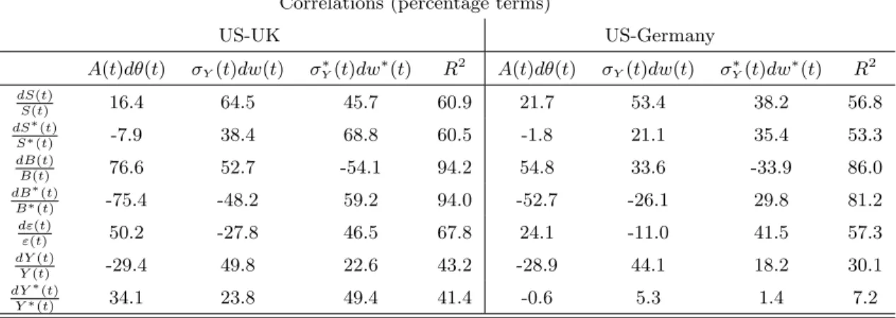
dS(t) S(t) = I1(t)dt + 1 − α αq(t) + 1 − αA(t)dθ(t) + αq(t) αq(t) + 1 − ασY(t)dw(t) + 1 − α αq(t) + 1 − ασ ∗ Y(t)dw∗(t) , (13) dS∗(t) S∗(t) = I2(t)dt − αq(t) αq(t) + 1 − αA(t)dθ(t) + αq(t) αq(t) + 1 − ασY(t)dw(t) + 1 − α αq(t) + 1 − ασ ∗ Y(t)dw ∗(t) , (14) dB(t) B(t) = I3(t)dt + 1 − α αq(t) + 1 − αA(t)dθ(t) − 1 − α αq(t) + 1 − ασY(t)dw(t) + 1 − α αq(t) + 1 − ασ ∗ Y(t)dw∗(t) , (15) dB∗(t) B∗(t) = I4(t)dt − αq(t) αq(t) + 1 − αA(t)dθ(t) + αq(t) αq(t) + 1 − ασY(t)dw(t) − αq(t) αq(t) + 1 − ασ ∗ Y(t)dw∗(t) , (16) dq(t) q(t) = I5(t)dt + A(t)dθ(t) − σY(t)dw(t) + σY∗(t)dw∗(t) , (17)
where θ(t) ≡ θH(t)/θF(t), A(t) ≡ λHλF(aH− aF)/[(λHθ(t)aH+ λFaF)(λHθ(t)(1 − aH) + λF(1 − aF))],
and Ij(t), j = 1, . . . , 5 are reported in the Appendix. Furthermore, if aH > aF, the diffusion
coefficients of the dynamics of the Home and Foreign stock markets and the terms of trade have the following signs: Variable/ Effects of dθ(t) dw(t) dw∗(t) dS(t) S(t) + + + dS∗(t) S∗(t) − + + dB(t) B(t) + − + dB∗(t) B∗(t) − + − dq(t) q(t) + − + (18)
Proposition 1 identifies some important interconnections between the financial and real markets in the world economy. Under the home bias assumption, it entails unambiguous directions of contemporaneous responses of all markets to innovations in supply and demand, summarized in (18). (18) nests some fundamental implications from various strands of international economics, which we highlighted in our earlier discussion. Our goal is to unify them within a simple model, and focus on the interactions.
One such interaction sheds light on the determinants of financial contagion − a puzzling ten-dency of stock markets across the world to exhibit excessive co-movement (for a recent detailed account of this phenomenon, see Kaminsky, Reinhart, and V´egh (2003)). Contagion in our model occurs in response to an output shock. Ceteris paribus, a positive output shock say in Home causes a positive return on the domestic stock market. At the same time, however, it initiates a Ricar-dian response of the terms of trade: the terms of trade move against the country experiencing a productivity increase. A flip side of the deterioration of the terms of trade in Home is an im-provement of those in Foreign. Hence, the value of Foreign’s output has to rise, thereby providing
a boost to Foreign’s stock market. Note that nothing in this argument relies on the correlation between the countries’ output processes. In fact, in a special case of our model where there are no demand shocks (discussed below), we obtain a perfect co-movement of the stock markets despite independence of the countries’ output innovations. Bond markets certainly also react to changes in productivity: a positive output shock in Home lowers bond prices in Home and lifts those in Foreign.
While supply shocks move the countries’ stock prices in the same direction, demand shocks act in the opposite way. We call this phenomenon “divergence.” Thus, a demand shock say in Home causes a relative demand shift biased toward the Home good, thereby boosting Home’s terms of trade. Improved terms of trade increase the value of Home’s output, and hence lift Home’s stock market, while decreasing that of Foreign’s output and lowering Foreign’s stock market. Similarly, since our bonds are real bonds, a strengthening of Home’s terms of trade increases the value of the Home bond and decreases that of the Foreign. A world economy without supply shocks is thus an example of perfect divergence: asset markets of different countries always move in opposite directions.
Finally, Proposition 1 provides analytical characterization of the sensitivities of each market’s responses to the supply and demand shocks, and also establishes cross-equation restrictions on how these sensitivities measure up to each other. The system of simultaneous equations describing the joint dynamics of the five markets (13)–(17) establishes a basis for our empirical analysis, carried out in Section 3.
2.3. Special Cases and Interpretations of θH and θF
In Proposition 1 we did not commit to specifying the dynamics of the demand shocks θH and θF. For the empirical analysis to follow, this is advantageous because the relative demand shock θ = θH/θF, in general, depends on the underlying Brownian motions w and w∗ inducing a correlation in the error structure that we do not have to impose ex-ante. In this section, we put more structure on the martingales θH and θF as we consider various economic interpretations of these processes:
dθH(t) = ~κH(t)>θH(t)d ~w(t) , dθH(t) = ~κF(t)>θH(t)d ~w(t) . (19)
A. Deterministic Preference Parameters
~κF are zeros. By substituting equation (8) into equation (12), we find that
S∗(t) = λHθH(0)aH+ λFθF(0)aF λHθH(0)(1 − aH) + λFθF(0)(1 − aF)
S(t).
As the multiplier term is non-stochastic, the two stock markets must be perfectly correlated. This implication achieves our goal of generating international financial contagion without assuming cor-relation between individual countries’ output processes, but it is certainly rather extreme and is easily rejected empirically. (Zapatero (1995) and Cass and Pavlova (2003) obtain this implication in their models as well, dubbing the resulting equilibrium a “peculiar” financial equilibrium.) In what follows, we force θH and θF to be stochastic processes, which would provoke the divergence effect and hence guarantee imperfect correlation between Home and Foreign stock markets, but would still produce financial contagion.
B. Preference Shocks or Pure Sentiment
The next special case we consider is where θH and θF are driven by the Brownian motion wθ, independent of w and w∗. In this case, ~κ
H = (0, 0, κH)> and ~κF = (0, 0, κF)>, where κH and κF are arbitrary adapted processes. Then θ has dynamics
dθ(t) = (κF(t)2− κH(t)κF(t)) θ(t) dt + (κH(t) − κF(t)) θ(t) dwθ(t).
The process θ can then be interpreted as a relative preference shock or a shock to consumer sentiment.
C. “Catching up with the Joneses”/ Consumer Confidence
Consider the case where the processes θH and θF depend on the country-specific Brownian motions:
~κH = (κH, 0, 0)> and ~κF = (0, κF, 0)>, where κH, κF < 0 may depend on w and w∗.7 Home and Foreign consumers’ preferences then display “catching up with the Joneses” behavior (Abel (1990)). The “benchmark” levels of Home and Foreign consumers, θH and θF, are negatively correlated with aggregate consumption of their country, Y and Y∗, respectively. Positive news to local aggregate
consumption reduces satisfaction of the local consumer, as his consumption bundle becomes less attractive in an improved domestic economic environment. The implication of this interpretation
7The labels κ
H and κF are used just to save on notation, they need not be the same as in interpretation B. Note
that under this interpretation ~κH and ~κF do not depend on the Brownian motion wθ. This specification makes wθ
a sunspot in the sense of Cass and Shell (1983): it affects neither preferences nor aggregate endowments. There is then a potential problem with employing the planner’s problem in solving for equilibrium allocations because it only identifies nonsunspot equilibria. Since markets are dynamically complete in our economy, however, the sunspot immunity argument of Cass and Shell goes through.
for the relative demand shock, θ, is that
dθ(t) = κF(t)2θ(t) dt + κH(t) θ(t) dw(t) − κF(t) θ(t) dw∗(t), κH(t), κF(t) < 0.
That is, an innovation to θ is negatively correlated with the Home output shock and positively correlated with the Foreign shock.
An alternative kind of dependence of agents’ preferences on the country-specific output shock is a form of consumer confidence. The idea is that agents get more enthusiastic when their local economy is doing well and hence demand more consumption. Formally, preferences exhibiting consumer confidence are the same as those under catching up with the Joneses, except that κH(t), κF(t) > 0. D. Radon-Nikodym Derivatives Reflecting Heterogeneous Beliefs
The previous two special cases we considered assume that consumer preferences are state-dependent. State-dependence of preferences, however, is not necessarily implied by our specification (4)–(5). Under the current interpretation, the countries have state-independent preferences, but they differ in their assessment of uncertainty underlying the world economy. For example, Home residents may believe that the uncertainty is driven by the (vector) Brownian motion ~wH ≡ (wH, w∗H, wθH)> and Foreign residents believe that it is driven by ~wF ≡ (wF, w∗F, wFθ)>. All we require is that the “true” probability measure P and the country-specific measures H (Home) and F (Foreign) are equivalent; that is, they all agree on the zero probability events. Under their respective measures, the agents’ expected utilities are given by
Ei ·Z T 0 [ailog(Ci(t)) + (1 − ai) log(Ci∗(t))]dt ¸ , i ∈ {H, F },
where Eidenotes the expectation taken under the information set of agent i. Thanks to Girsanov’s
theorem, the above expectations can be equivalently restated under the true probability measure in the form of (4)–(5). The multiples θH and θF, appearing in the expressions as a result of the change of measure, are the so-called Radon-Nikodym derivatives of H with respect to P , ¡dHdP¢, and F with respect to P ,¡dF
dP
¢
, respectively.
The Radon-Nikodym derivatives θH and θF may reflect various economic scenarios. One is the case of incomplete information: the consumers do not observe the parameters of the output processes, and need to estimate them. While the diffusion coefficients σY(t) and σ∗Y(t) may be estimated by computing quadratic variations of Y (t) and Y∗(t), estimation of mean growth rates
with some priors of the growth rates. Then they will be updating their priors each instant as new information arrives, through solving a filtering problem.8 Second, the consumers may use some
updating method other than Bayesian. For example, they may be systematically overly optimistic or pessimistic about the mean growth rates of output. Finally, they may explicitly account for model uncertainty in their decision-making. All these special cases result in consumers employing a probability measure different from the true one. These differences of opinion can be succinctly represented by some Radon-Nikodym derivatives θH and θF. Under any of these interpretations, we can no longer assume that θ in Proposition 1 is uncorrelated with either w or w∗, which we have
to take into account in our econometric tests.
2.4. Interest Rate Parity and Trading Strategies
Uncovered interest rate parity in its classical form is a relationship between local interest rates at Home and Foreign and the expected exchange rate (terms of trade) appreciation. In this section we show that in our setting, such a relationship must have an additional term capturing a pertinent risk premium. This term is, in general, time-varying. We also fully characterize equilibrium interest rates prevailing at Home and Foreign, under different interpretations of the demand shocks. These results are reported in the following proposition.
Proposition 2. The uncovered interest rate parity relationship has the form rF(t) − µ
q(t) = rH(t) + σq(t)>(mH(t) + σq(t)), (20)
where µq and σq are the mean growth and volatility parameters in the dynamic representation of q,
dq(t)/q(t) = µq(t)dt + σq(t)>d ~w(t), mH is the Home market price of risk reported in the Appendix,
and rH and rF are the Home and Foreign real interest rates, i.e., instantaneously riskless returns
on local money market accounts specified in terms of the local goods, given by: (i) under interpretations A and B,
rH(t) = µ
Y(t) − σY(t)2, r
F(t) = µ∗
Y(t) − σ∗Y(t)2,
8We provide details of the ensuing filtering problems in the Appendix, in the context of the proof of Proposition 2.
We consider the case where the agents believe there are only two independent innovation processes, wi and wi∗, and
the case where, additionally, there is the third one, wθ
i. The first two innovations drive the output processes Y
and Y∗, respectively. Following Detemple and Murthy (1994), we impose additional regularity conditions on σ
Y(t)
and σ∗
Y(t) to make the filtering problem tractable: both processes are bounded and are of the form σY(Y (t), t) and
σ∗
Y(Y
∗(t), t), respectively. When the agents perceive that the parameters they are estimating also depend on the
third innovation process, which can represent either intrinsic of extrinsic uncertainty (a sunspot), they make use of a public signal carrying information about wθ
(ii) under interpretation C, rH(t) = µ Y(t) − σY(t)2+ λHθH(t)aH λHθH(t)aH+ λFθF(t)aF | {z } CH(t)/YH(t) σY(t)κH(t), rF(t) = µ∗ Y(t) − σ ∗ Y(t) 2+ λFθF(t)(1 − aF) λHθH(t)(1 − aH) + λFθF(t)(1 − aF) | {z } C∗ F(t)/YF∗(t) σY∗(t)κF(t),
(iii) under interpretation D (see the Appendix for the detailed description of the economic setting), rH(t) = µ Y(t) − σY(t)2+ λHθH(t)aH(µH(t) − µY(t)) + λFθF(t)aF(µF(t) − µY(t)) λHθH(t)aH+ λFθF(t)aF | {z } CH (t) Y (t) (µH(t)−µY(t))+CF (t)Y (t) (µF(t)−µY(t)) , rF(t) = µ∗ Y(t) − σ ∗ Y(t) 2+λHθH(t)(1 − aH)(µ∗H(t) − µY∗(t)) + λFθF(t)(1 − aF)(µF(t) − µ∗Y(t)) λHθH(t)(1 − aH) + λFθF(t)(1 − aF) | {z } C∗H(t) Y ∗(t)(µ∗H(t)−µ∗Y(t))+ C∗F(t) Y ∗(t)(µ∗F(t)−µ∗Y(t)) ,
where µH(t) and µF(t) denote perceived or estimated mean growth rates of the Home output by
Home and Foreign consumers, respectively, and µ∗
H(t) and µ∗F(t) denote perceived or estimated
mean growth rates of the Foreign output by Home and Foreign consumers, respectively.
In its classical form, uncovered interest rate parity is a relationship which assumes that arbitrage will enforce equality of returns on the following two investment strategies. The first one is investing a unit of wealth in the Home money market account resulting in receiving the riskless return at rate rH, in units of the Home good, over the next instant. The second is investing the same amount in the Foreign money market, at rate rF, over the next instant and then converting the proceeds paid out in the Foreign good into the Home good using the prevailing terms of trade. In our model, the two strategies are not equivalent because in terms of the Home good, the first strategy is riskless, while the second one is risky. The left-hand side of (20) represents the mean return on the second strategy, given by the Foreign money market rate less the mean terms of trade appreciation. The right-hand side contains the return on the riskless first strategy, plus an additional term capturing the risk premium the risky strategy commands. This risk premium is, in general, time-varying. The only case in which it can be shown to be constant in the context of our model is within interpretation A (no demand shocks) under an additional assumption that the mean growths and volatilities of the output processes Y and Y∗ are constant. Recall that the
Under the remaining interpretations, the risk premium term depends on the demand shocks. Hence, uncovered interest rate parity in its classical form − (20) with no risk premium term − does not obtain in our model.
In the empirical section, which comes next, we estimate the variance-covariance matrix of the shocks, and find that the variance of demand shocks is two times larger than that of supply shocks. One implication of this finding is that the risk premium would be very volatile, too. Deviations from the classical uncovered interest rate parity relationship have been found to be very large and volatile, and the need for a very volatile risk premium has been emphasized repeatedly in the empirical literature since Fama (1984). Our model may then shed some light on these issues.
Equilibrium riskless rates of return on money market accounts in each country have to be such that agents are willing to save. In the benchmark case of no demand shocks (interpretation A), local interest rates must then be positively related to the growth of aggregate consumption of the local good and negatively related to the aggregate consumption volatility, reflecting the precautionary savings motive. When the demand shocks are interpreted as pure sentiment shocks (B), driven by an independent source of uncertainty, the local money market rates are the same as in the benchmark. This is because the sentiment shocks are martingales; otherwise if they had nonzero mean growth terms, these terms would have appeared in the expression for the interest rate as additional inducements for the agents to save, acting analogously to impatience parameters (which we do not model). Since the demand shocks do not co-vary with aggregate consumption uncertainty, they also do not give rise to an additional precautionary savings component. Such a component appears under interpretation C, where aggregate consumption of the local good imposes a negative (catching up with the Joneses) or positive (consumer confidence) externality on the agents. In the former case, this gives rise to an additional precautionary savings effect, driving down the interest rates, while in the latter case the interest rates rise. The strength of this additional effect induced by consumption externalities of Home (Foreign) agents is determined by the relative importance of Home (Foreign) consumers in the world economy. This relative importance is captured by the shares of the agents in the aggregate consumption of the local good, which can also be linked to wealth distribution in the economy. An additional component over the benchmark also appears in the interest rate expressions under the differences of opinion interpretation D, as highlighted in Proposition 2. Perhaps a better way to present say the Home rate under this interpretation is as a weighted average of the Home rates prevailing if only Home consumers were present in the economy
(µH(t) − σY(t)2) and if only Foreign consumers were present (µF(t) − σY(t)2), with weights again given by the agents’ consumption shares.
We now turn to computing the agents’ trading strategies. To facilitate comparison with the literature, we consider an additional security: a “world” bond BW, locally riskless in the numeraire. This bond does not, of course, introduce any new investment opportunities in the economy; it is just a portfolio of α shares of the Home bond and (1-α) shares of the Foreign bond. Let r denote the interest rate on this bond.
The number of non-redundant securities differs across interpretations A–D, which complicates our exposition. Thus, as we discussed earlier, Home and Foreign stocks are perfectly correlated under interpretation A, and hence investments in individual stock markets cannot be uniquely determined. Under the remaining interpretations, we can uniquely identify agents’ holdings of national stock markets. One of the bond markets, however, may or may not be redundant depending on the interpretation. In what follows, we replace the Foreign bond by the world bond in the investment opportunity set of the agents. (Investment in the Foreign bond can be recovered from the portfolio allocations to the Home and world bonds, where applicable.)
Before we proceed to reporting our results, we need to define the notion of a home bias. We measure a bias in portfolios relative to the (common to the agents) mean-variance portfolio. Thus, a Home (Foreign) resident’s portfolio is said to exhibit a home bias if the portfolio weight he assigns to the Home (Foreign) stock is higher than that in the mean-variance portfolio.
Proposition 3. (i) Countries’ portfolios are given by xi(t) = (σ(t)>)−1I m(t) | {z } mean-variance portfolio + (σ(t)>)−1I ~κi(t) | {z } hedging portfolio , i ∈ {H, F } , (21)
where the compositions of the vector of the fractions of wealth invested in risky assets, xi, of the
volatility matrix of the investment opportunity set σ, of the market price of risk m and of the auxiliary matrix I, different across interpretations A–D, are provided in the Appendix. The remaining fraction of wealth, 1−x>
i~1, is invested in the world bond B
W, where ~1 = (1, . . . , 1)>.
(ii) Under interpretation B, countries’ portfolios do not exhibit a home bias. Assume further that aH > aF. Then, under interpretation C, in the case of κH(t), κF(t) > 0 (consumer
confi-dence) portfolios always exhibit a home bias, while in the case of κH(t), κF(t) < 0 (catching
up with the Joneses) the portfolio of Home exhibits a home bias if and only if (1 − α)σ∗
Y(t) +
A(t)θ(t)αq(t)κF(t) > 0 and that of Foreign if and only if αq(t)σY(t)+A(t)θ(t)(1−α)κH(t) > 0.
(iii) The international CAPM has the form Et(dSj(t)) Sj(t) − r(t) = Covt µ dSj(t) Sj(t) , dW (t) W (t) ¶ − Covt µ dSj(t) Sj(t), λH λHθH(t) + λFθF(t) dθH(t) ¶ −Covt µ dSj(t) Sj(t) , λF λFθF(t) + λFθF(t) dθF(t) ¶ , Sj∈ {S, S∗} , (22)
where W ≡ WH + WF is the aggregate wealth and r is the interest rate on the world bond,
reported in the Appendix.
In our economy, the fact that the countries have logarithmic preferences does not imply that the their investment behavior is myopic. Their trading strategies involve holding the standard mean-variance portfolio along with a hedging one. Although the countries do not hedge against changes in the investment opportunity set (which is standard for logarithmic preferences), they do hedge against their respective demand shocks.9 The way they do so depends on the correlation
between their demand shocks and output shocks, and hence differs across our interpretations of demand shocks. Thus, if the demand shocks are independent of output shocks − pure sentiment interpretation B − portfolio weights the countries assign to the stocks coincide with those in the mean-variance portfolio. If a country’s demand shocks are positively related to its output shocks (consumer confidence interpretation C)− that is, if a country demands more consumption (biased toward the domestic good) when it is experiencing a positive output shock − consumers increase their portfolio holdings of the domestic stock, a claim to domestic output. On the other hand, if the demand shocks are negatively correlated with the country’s output innovations − catching up with the Joneses interpretation C − a home bias in portfolios may or may not arise. Proposition 3 provides a necessary and sufficient condition for the bias to occur. Finally, our differences of opinion interpretation D is too general to entail unambiguous implications on the sign of the bias. However, if specialized further, it is likely to yield sharper predictions. For example, albeit in a different setting, Uppal and Wang (2003) argue that disparities in agents’ ambiguity about home and foreign stock returns can lead to a home bias in portfolios.
9Our references to consumers’ hedging behavior made in the context of the differences of opinion interpretation
of the demand shocks may appear confusing. How can consumers hedge deviations of their beliefs from the true probability measure, which they do not know? In fact, they do not. They hold a portfolio which is mean-variance efficient under their own probability measure, given by the product of the inverted volatility matrix (σ>)−1 and the
country-specific market prices of risk mi = m + ~κi, constructed from their own investment opportunity sets. The
representation in equation (21) is thus formally equivalent to a mean-variance portfolio under a country’s individual beliefs, except it further decomposes a country-specific market price of risk into two components: the “true” market price of risk m and the measure of deviation of agent’s beliefs from the true probability measure ~κi, both unobservable
The presence of the hedging portfolios optimally held by the agents clearly rules out the tradi-tional one-factor CAPM. In addition to the standard market (aggregate wealth) factor, our model identifies two further factors, the Home and Foreign demand shocks, that affect the risk premia on the stocks. The expression in (22) also differs from the international CAPM (see Solnik (1974), Adler and Dumas (1983)). As is standard for logarithmic preferences, the exchange rate does not appear explicitly in (22); however, its determinants − the demand shocks − do. (One would expect the exchange rate to appear as an additional factor if we relaxed the assumption of logarithmic preferences.) The presence of the demand shocks points to a possible misspecification of the CAPM widely tested empirically. Our alternative formulation might then provide an improvement over the standard specification used in the international finance literature.
3.
Empirical analysis
In this section we examine the empirical implications of the model. We use daily data for the US vis-`a-vis the UK and Germany that has been collected from DataStream. As proxies for our riskless bonds, we use data on the three-month zero-coupon government bonds for each country. The US, UK and German stock market indexes are taken to represent the countries’ stock prices. The dollar-pound and dollar-mark exchange rates are used for identifying the real exchange rates and the terms of trade via a procedure described below. The data for the US and the UK are from 1988 until the end of 2002. The data for Germany is shorter, until December 1998, because of the transition to the euro. We did not consider it prudent to complete the data from 1998 to the end of 2002 by extrapolating the euro exchange rates and interest rates to the mark. Moreover, we do not want our exercise to be contaminated by the change in an exchange rate regime that took place with the creation of the euro. All empirical analysis involving Germany is thus performed on a shorter data set.
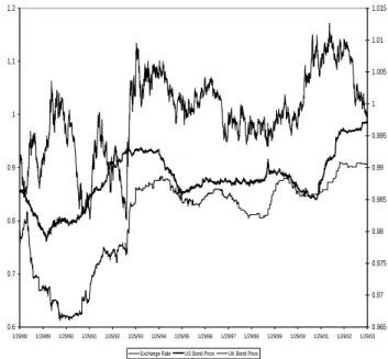
Figure 1 depicts the evolution of the exchange rate along with stock and bond markets values for the US vis-`a-vis Germany and the UK. Even a casual observation of the figure suggests that the bond prices do not bear too much relationship to the exchange rates. This observation is strongly supported by a regression analysis, not reported here, whose results may be interpreted as a failure of uncovered interest rate parity, well-documented in the literature and also found in our sample. On the other hand, the amount of co-movement between the stock indexes and the exchange rates is quite striking. We computed the pertinent correlations and found them to be highly statistically
significant. Our theory that stock prices and exchange rates are driven by the same set of factors, then, does not appear to be empirically unfounded.
3.1. Real and Nominal Quantities
Before we proceed with our formal empirical analysis, we need to establish a mapping between the quantities employed in our model and those in the data available to us − the data are in nominal terms, while our model is real. The main issue is to impute the terms of trade from the available data on nominal exchange rates. To do so, we first compute the real exchange rate implied by our model. The real exchange rate, e, is defined as e(t) = PH(t)/PF(t), where PH and PF are Home and Foreign price indexes, respectively. In practice, a variety of methods have been used for computing a country’s price level, or cost of living (see Schultze (2003)). We have chosen to adopt geometric average price indexes, which address the criticism pertaining to the substitution between goods bias, and are consistent with the countries’ homothetic preferences:
PH(t) = µ p(t) aH ¶aHµ p∗(t) 1 − aH ¶1−aH , PF(t) = µ p(t) aF ¶aFµ p∗(t) 1 − aF ¶1−aF . The real exchange rate, expressed as a function of the terms of trade, is then
e(t) = q(t)aH−aF (1 − aF)
1−aFaaF F (1 − aH)1−aHaaHH
.
Finally, to obtain the nominal exchange rate, we need to adjust the real exchange rate for inflation in Home versus Foreign. Unfortunately, daily data on inflation, required for our estimation, are not available. However, our data span a relatively short period of time when international inflation rates were very low. Consequently, as argued by Mussa (1979), our real rates are closely related to the nominal ones. We thus assume that inflation is negligibly small and simply make a level adjustment to the real rate to back out the nominal exchange rate, ε: ε(t) = εe(t), where ε is the average nominal exchange rate in the sample.
For our empirical investigation of the dynamics reported in Proposition 1, we use the variable q(t) = µ ε(t) ε (1 − aH)1−aHaaHH (1 − aF)1−aFaaFF ¶1/(aH−aF) (23) as a proxy for the terms of trade. Taking logs and applying Itˆo’s lemma, we obtain an equation to replace (17) in Proposition 1: dε(t) ε(t) = I6(t)dt + (aH− aF)A(t)dθ(t) − (aH− aF)σY(t)dw(t) + (aH− aF)σ ∗ Y(t)dw ∗(t) ,
where I6(t) = (aH−aF)I5(t)+12(aH−aF)(aH−aF−1)|σq(t)|2. Under our assumption of no inflation over the time period we are considering, the remaining equations in Proposition 1, (13)–(16), are unchanged when prices are expressed in nominal terms. Finally, since the nominal exchange rate, ε, is monotonically increasing with the terms of trade q, the signs of the coefficients identified in Proposition 1 are maintained for nominal prices. Moreover, the signs of the effects of the shocks
on dε(t)ε(t) are the same as those for dq(t)q(t) reported in (18).
For a practical implementation of this conversion of units, we need to calibrate parameters aH, aF and α used in the expressions. It is reasonable to assume that about three quarters of a country’s consumption comes from the locally produced good. Such home bias is primarily due to the presence of non-tradable goods, which comprise a large fraction of national consumption. While we do not explicitly account for non-tradable goods, their presence is modeled in reduced form, through parameters aH and aF (see Section 4 for further elaboration). It is thus reasonable to set aH equal to 0.75 and aF equal to 0.25. We also need a sensible value for α, the weight of the US-produced goods in the world numeraire basket, or a price index. By setting α = 0.75 we are implicitly assuming that the US economy is about three times the UK economy. Of course, we run robustness checks where we vary these parameters, which we discuss later in this section. The calibrated values of aH and aF are used for computing the series for the terms of trade via (23). We then use the numeraire basket (identified by α) and the terms of trade to convert stock and bond prices for each country into a common numeraire.
3.2. Cross equation restrictions
We now turn to testing our model’s implications on the dynamic behavior of asset prices and exchange rates. They are summarized in Proposition 1, in the system of equations (13)–(17) and the accompanying table with the predicted signs of the coefficients (18). For convenience, we reproduce this system below, in a matrix form:
dS(t) S(t) dS∗(t) S∗(t) dB(t) B(t) dB∗(t) B∗(t) dε(t) ε(t) = ~I + b(t) 1 − b(t) b(t) −1 + b(t) 1 − b(t) b(t) b(t) −b(t) b(t) −1 + b(t) 1 − b(t) −1 + b(t) (aH− aF) − (aH− aF) (aH− aF) | {z } B1 A (t) dθ (t) σY(t) dw (t) σ∗ Y (t) dw∗(t) , (M1)
where ~I is a (vector) intercept term and b(t) ≡ 1 − α αq (t) + 1 − α, with q(t) = µ ε(t) ε (1 − aH)1−aHaaHH (1 − aF)1−aFaaFF ¶1/(aH−aF) . (24)
Unfortunately, while we can construct all the left-hand side variables in (M1), we do not have data on the variables on the right-hand side of the system. Consequently, in our estimation we treat the innovations A (t) dθ (t), σY (t) dw (t), and σ∗Y(t) dw∗(t) as latent factors that we extract from stock and bond prices and exchange rates. The first factor, A (t) dθ (t), captures the relative demand shock, while the remaining two, σY(t) dw (t) and σ∗Y(t) dw∗(t), represent Home and Foreign supply shocks, respectively. (There is a slight abuse of terminology in this section; earlier we referred to dθ, dw and dw∗ as the demand and supply shocks.) Note that the factor loadings in matrix B
1 are
fully described by the quantity b(t), which depends only on the weight of the US-produced goods in the world numeraire basket α, the nominal exchange rate ε, and the preference for domestic good parameters aH and aF.
Perhaps the most direct approach to testing our model would be to take Proposition 1 literally and estimate the structural latent factor model (M1). Note, however, that since the factors are in general heteroskedastic and may be correlated in our model, a priori there is no reason to put any restrictions on their variance-covariance matrix. The only set of restrictions our theory entails is those on the elements of matrix B1. This estimation strategy, in practice, imposes too few
constraints on the model: implicitly, we would be fitting five series with three unrestricted factors. As a result, the fit of the model within sample would be very good and the likelihood of rejecting the model very low.10 For this reason, we have decided to adopt a different approach. We seek support
for our theoretical implications from the following two tests. The first one considers a simplified version of (M1), where factor loadings are assumed constant, and the factors are homoskedastic. We impose all the cross equation constraints, i.e., force the factor loadings in B1 to be related to
each other exactly as specified. In the second test, we drop the cross equations restrictions as well as the assumption of homoskedasticity of the factors, and estimate the model imposing only the sign restrictions from (18). The remainder of this subsection implements the first test, and the next subsection is devoted to the second one.
The key to executing the first test is recognizing that under the assumptions of constant coeffi-cients (b(t) = b) and homoskedasticity we can estimate the model using the unconditional covariance
10We have indeed estimated the model following this strategy. The fit within sample has been unrealistically good.
US-UK US-Germany
Point Estimate Std. Error Point Estimate Std. Error
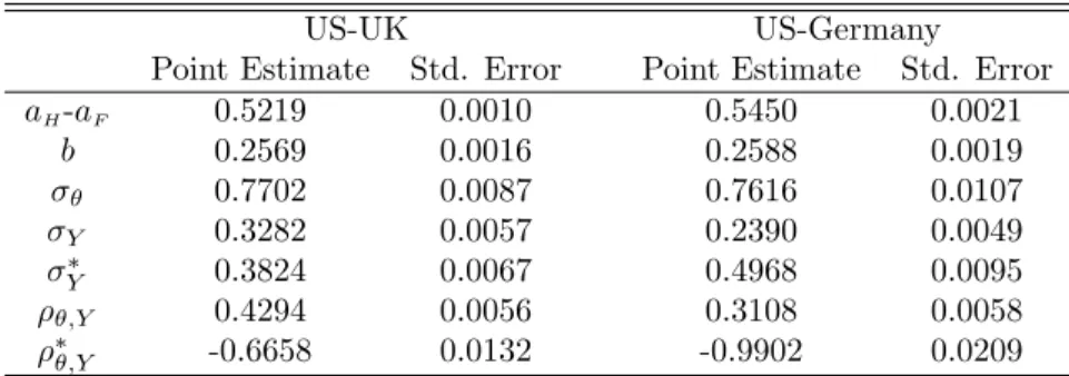
aH-aF 0.5219 0.0010 0.5450 0.0021 b 0.2569 0.0016 0.2588 0.0019 σθ 0.7702 0.0087 0.7616 0.0107 σY 0.3282 0.0057 0.2390 0.0049 σ∗ Y 0.3824 0.0067 0.4968 0.0095 ρθ,Y 0.4294 0.0056 0.3108 0.0058 ρ∗ θ,Y -0.6658 0.0132 -0.9902 0.0209
Table 1: Constant coefficients and cross equation restrictions: Estimation of Model (M1) for the US vis-`a-vis the UK and Germany. σθ denotes the standard deviation of the
relative demand shock A(t)dθ(t), and ρθ,Y, ρ∗θ,Y are the correlations of this factor with the supply
shocks σY(t)dw(t) and σY∗(t)dw∗(t), respectively. All standard deviations are in percentage terms. matrix computed from the aforementioned five time series for each pair of countries. We allow the covariance matrix of the factors to be non-diagonal, so that the test can incorporate all of our interpretations of θ and suggest which ones appear plausible in the data. We still force the two supply shocks to have a covariance of zero, but the other two covariance terms are allowed to differ from zero. We estimate the coefficients b and aH-aF, and the covariance matrix by GMM. We have 15 second moments estimated from the data (the covariance matrix of the observed returns), which have to be explained by seven coefficients: two coefficients identifying matrix B1, b and aH-aF, and five coefficients describing the covariance matrix of the latent factors (three variances and two correlations). The results are reported in Table 1.
Consider first the case of the US vis-`a-vis the UK. As we discussed earlier, the reasonable calibration of parameters aH and aF are 0.75 and 0.25, respectively. The point estimate of aH-aF, 0.5219, is then very close to the calibrated value. Furthermore, after our accounting for the level effect of the nominal exchange rate and the calibration of α, the average value of the terms of trade from (23) is, roughly, one. Then, the calibrated value of the coefficient b from (24) is about 0.25. The estimate we obtain in the data is 0.2569 − very close indeed.
The remaining five estimates summarize the covariance matrix of the three latent factors. First, note that the demand shocks are very important both in magnitude and significance, rejecting our interpretation A, where we assume that only the supply shocks drive the economy. In fact, the standard deviation of the demand shocks is twice as large as that of the supply shocks. The standard deviations of the two supply shocks have similar orders of magnitude. Second, note that the estimates of the correlations constructed from the covariance matrix, indicate that the relative demand shock is positively correlated with the US’s supply shock, and negatively correlated
with the UK’s. The estimates are statistically significant, strongly rejecting the pure sentiment interpretation B. Furthermore, the catching up with the Joneses interpretation C, under which the the relative demand shock should negatively co-vary with the US supply shock and positively with the UK’s, is rejected, too. The story the data is telling is the reverse: instead of becoming relatively unhappy when their country’s aggregate consumption increases, agents appear to get enthusiastic when their economy is doing well. This speaks in favor of our consumer confidence interpretation C. Alternatively, these results may be viewed as evidence of differences in opinion (interpretation D).
The results for the case of the US vis-`a-vis Germany are very similar. The point estimates of aH-aF and b are almost identical to the previous case, as one would expect because the relative sizes of the economies and their preference biases toward domestic goods are close. The variances are also similar, although, in the case of Germany, its supply shocks are larger than the UK’s. The pattern of the correlations is close to the previous case: again, the relative demand shock is positively correlated with the US supply innovations, and negatively correlated with the German − in support of the consumer confidence interpretation.
In summary, the structural parameters estimated in this exercise are close to those from cali-bration of B1. Furthermore, we find that demand shocks are very important in explaining short-run
variation of asset prices: their variance is twice the size of that of supply shocks. Furthermore, in the data demand shocks are neither independent of supply shocks, nor support the catching up with the Joneses interpretation. Rather, the demand shocks are due to either differences of opinion or variations in consumer confidence, positively related to fluctuations in national output.
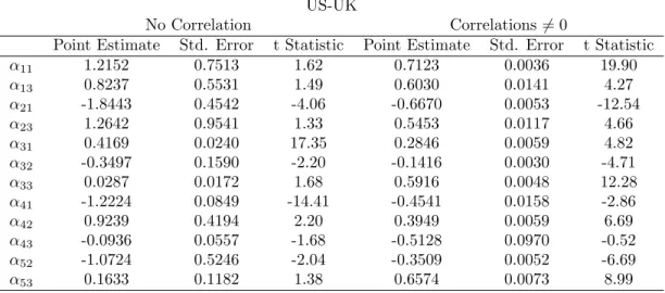
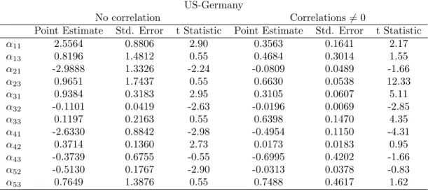
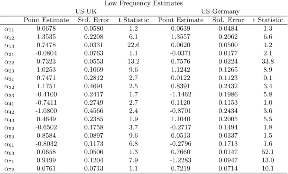
3.3. Sign Restrictions
The previous section studied a very restrictive version of the model. In this section we relax the cross equation restrictions on the coefficients of matrix B1, and also allow the variance of the latent
factors to change through time. We continue to maintain the assumption that the coefficients are constant, but now impose only the sign restrictions arising from Proposition 1. Indeed, one of the principal implications of the model is the unambiguous prediction for the signs of the responses of observed prices to innovations in the latent factors, summarized in (18). We thus estimate the