Analysis of the diurnal behavior of Evaporative Fraction
by
Pierre Gentine
Dipl. Ing. in Aerospace Engineering Sup'Aero, Toulouse, FRANCE
Submitted to the Department of Civil and Environmental Engineering
in partial fulfillment of the requirements for the degree of
Master of Science in Civil and Environmental Engineering
at the
MASSACHUSETTS INSTITUTE OF TECHNOLOGY
June 2006
@
Massachusetts Institute of Technology 2006. All rights reserved.
Author... ...
Department of Civil and Environmental Engineering
April 16, 2006
Certified by...
Professor of
Dara Entekhabi
Civil and Environmental Engineering
Thesis Supervisor
I1
IAccepted by ...
Andrew Whittle
Chairman, Departmental Committee for Graduate Students
MASSACHUSETTS INSTiTUTE OF TECHNOLOGY
BARKER
JUN E
7 2006
Analysis of the diurnal behavior of Evaporative Fraction
by
Pierre Gentine
Dipl. Ing. in Aerospace Engineering Sup'Aero, Toulouse, FRANCE
Submitted to the Department of Civil and Environmental Engineering
on April 16, 2006, in partial fulfillment of the
requirements for the degree of
Master of Science in Civil and Environmental Engineering
Abstract
In this thesis, the diurnal behavior of Evaporative Fraction (EF) was
examined. EF was shown to exhibit a typical concave-up shape, with a
minimum usually reached in the middle of the day. The influence of the
vegetation cover and the soil moisture conditions on EF diurnal shape
was also investigated. We also checked the repercussion of a change in
environmental conditions on EF. This study will finally allow a better
understanding of EF and suggests some new methods to obtain a good
estimate of EF and of evapotranspiration.
Thesis Supervisor: Dara Entekhabi
Acknowledgments
First, I would like to convey my appreciation to the whole SUDMED project team. They provided the data set necessary to make this thesis possible, and I had a invaluable experience working with them in Marrakech, Morocco.
Then, I would like to sincerely thank my thesis advisor, Professor Dara Entekhabi, for his amazing advice and ideas. I also would like to thank him for being so nice with any student, and respecting their ideas and point of view. I really enjoyed working
with him.
Finally, I would like to warmly thank Marie, my family and Onur. They gave me the energy to overcome any moments.
Contents
1
SUDMED project and main sites 171.1 Sites description . . . . 17
1.1.1 A gdal site . . . . 19
1.1.2 R 3 site . . . . 19
1.2 Experimental data set . . . . 20
1.2.1 A gdal site . . . . 20
1.2.2 R 3 site . . . . 21
1.3 Calibration and validation of the SVAT model . . . . 23
1.3.1 C alibration . . . . 23
1.3.2 R 3 site . . . . 24
1.3.3 A gdal site . . . . 25
2 Frequency analysis of EF 27 2.1 Frequency analysis of EF . . . . 27
2.1.1 Fast Fourier Transform (FFT) . . . . 27
2.1.2 Fast Fourier Transform (FFT) on moving window . . . . 27
2.1.3 Lomb periodogram . . . . 28
3 Analysis of EF diurnal behavior 31 3.1 Article submitted to Agricultural and Forest Meteorology . . . . 31
3.2 Complementary results and discussion . . . . 85
3.2.2 Variation of sensible and latent heat fluxes with soil moisture and L A I . . . . 88 4 EF models 91 4.1 Combined-source EF modeling . . . . 92 4.2 Dual-source EF modeling . . . . 95 A Tables 99 B Figures 103
List of Figures
B-i M ap of M orocco ... 104 B-2 Solar incoming radiation measured over parcel R3-B123 in 2003 . . . 105
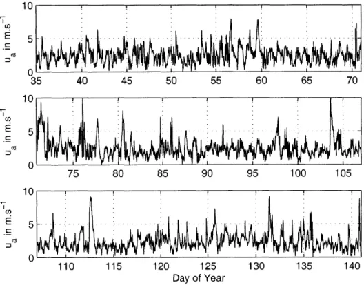
B-3 Air temperature measured over parcel R3-B123 in 2003 . . . . 106 B-4 Air specific humidity measured over parcel R3-B123 in 2003 . . . . . 107 B-5 Wind speed measured over parcel R3-B123 in 2003 . . . . 108 B-6 Net radiation measured at 2m high over parcel R3-B123 in 2003 . . . 109
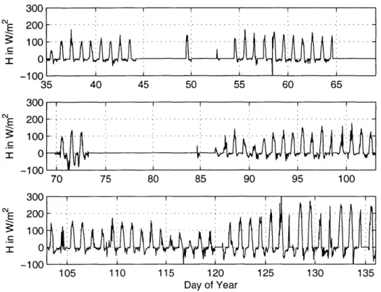
B-7 Sensible Heat Flux measured using Eddy-Correlation over parcel R3-B 123 in 2003 . . . . 110 B-8 Latent Heat Flux measured using Eddy-Correlation over parcel
R3-B 123 in 2003 . . . . 111 B-9 Mean ground heat flux measured using 3 flux plates over parcel
R3-B 123 in 2003 . . . . 112
B-10 Frequency analysis of latent heat flux using Lomb periodogram . . . . 113
B-11 Reconstructed latent heat flux using Lomb periodogram . . . . 114 B-12 Daytime and Midday Evaporative Fraction (EFd and EFm) as a
func-tion of Solar incoming radiafunc-tion in W.m. . . . .. 115
B-13 Daytime and Midday Evaporative Fraction (EFd and EFm) as a func-tion of wind speed in m .s.. . . . . 116
B-14 Cross-correlation of EF and air relative humidity, for LAI=0.5, 1.5, 2.5 and 3.5 and surface soil moisture between 0.1 and 0.4 m3m 3 . . . . 117
B-15 Cross-correlation of EF and air specific moisture, for LAI=0.5, 1.5, 2.5 and 3.5 and surface soil moisture between 0.1 and 0.4 m3.m-3 . . . . 118
B-16 Daytime and Midday Evaporative Fraction (EFd and EFm) as a func-tion of air specific humidity in gH20/kgair . . . . . . . . . . . . 119 B-17 Daytime and Midday Evaporative Fraction (EFd and EFm) as a
func-tion of air temperature in C. . . . . 120 B-18 Daytime and Midday Evaporative Fraction (EFd and EFm) as a
func-tion of L A I. . . . . 121 B-19 Daytime and Midday Evaporative Fraction (EFd and EFm) as a
func-tion of vegetafunc-tion height. . . . . 122 B-20 Daytime and Midday Evaporative Fraction (EFd and EFm) as a
func-tion of roughness length. . . . . 123
B-21 Daytime and Midday Evaporative Fraction (EFd and EFm) as a func-tion of the ratio between the momentum roughness length and the heat roughness length. ... ... 124 B-22 Mean diurnal value of sensible heat flux H as a function of surface soil
moisture for LAI=0.5, 1.5, 2.5, 3.5 and 4.5. . . . . 125
B-23 Mean diurnal cycle of a) sensible heat flux, b) soil sensible heat flux and c) canopy sensible heat flux for LAI=0.5, 2.5 and 4.5 and surface soil moisture 0, =0.1, 0.2, 0.3 m3.m . . . . 126
B-24 Mean diurnal value of latent heat flux as a function of surface soil moisture for LAI=0.5, 1.5, 2.5, 3.5 and 4.5. . . . . 127
B-25 Mean diurnal value of soil heat flux G as a function of surface soil moisture for LAI=0.5, 1.5, 2.5, 3.5 and 4.5. . . . . 128
B-26 Cumulative absolute ET error in mm as a function of surface soil mois-ture for LAI=0.5, 1.5, 2.5, 3.5 and 4.5. . . . . 129 B-27 Cumulative absolute ET error in percent of total cumulative ET as a
function of surface soil moisture for LAI=0.5, 1.5, 2.5, 3.5 and 4.5. . . 130
B-28 Cumulated ET estimation error for different models ft ETmodel(t)
-ETsVAT(t) dt in mm as a function of mean surface soil moisture for
B-29 Min/Max (dotted line) and mean (solid line) evapotranspiration error
tnd ETo (t) - ET(t) dt in mm, when using the constant EF
assump-tion and measuring EF at different hour of the day between lOAM and 4PM, as a function of mean surface soil moisture for a) LAI=1, b)
LAI=2, c) LAI=3, d) LAI=4. . . . . 132
B-30 Min/Max (dotted line) and mean (solid line) evapotranspiration error
ftend ETo2(t) - ET(t) dt in mm, when using the constant EF'
assump-tion and measuring EF' at different hour of the day between lOAM and 4PM, as a function of mean surface soil moisture for a) LAI= 1, b)
LAI=2, c) LAI=3, d) LAI=4. . . . . 133
B-31 Cumulated evapotranspiration estimation error for different models
tend ETmodel(t) - ETSVAT(t) dt in percents as a function of mean
sur-face soil moisture for LAI=1, 2, 3 and 4. . . . . 134 B-32 Min/Max (dotted line) and mean (solid line) evapotranspiration error
f
tend EToi (t) - ETsVAT(t) dt in percents, when using the constant EFassumption and measuring EF at different hour of the day between 10AM and 4PM, as a function of mean surface soil moisture for a)
LAI=1, b) LAI=2, c) LAI=3, d) LAI=4. . . . . 135
B-33 Min/Max (dotted line) and mean (solid line) evapotranspiration error
ftend ETo2(t) - ETsVAT(t) dt in percents, when using the constant EF' assumption and measuring EF' at different hour of the day between 10AM and 4PM, as a function of mean surface soil moisture for a)
LAI=1, b) LAI=2, c) LAI=3, d) LAI=4. . . . . 136
B-34 First and second best evapotranspiration forecasting models as a func-tion of surface soil moisture . . . . 137 B-35 First and second worst evapotranspiration forecasting models as a
func-tion of surface soil moisture . . . . 138 B-36 Cumulated evapotranspiration estimation error for different models
f
tn ETmodel(t) - ETsVAT(t) dt in mm as a function of mean surfaceB-37 Min/Max (dotted line) and mean (solid line) evapotranspiration error
f tend
EToi (t)
-ET(t) dt
in mm, when using the constant EFassump-tion and measuring EF at different hour of the day between 10AM and 4PM, as a function of mean surface soil moisture for a) LAI=1, b)
LAI=2, c) LAI=3, d) LAI=4. . . . . 140
B-38 Min/Max (dotted line) and mean (solid line) ET error ft ET02
(t)
-ET(t) dt in mm, when using the constant EF' assumption andmea-suring EF' at different hour of the day between 10AM and 4PM, as a function of mean surface soil moisture for a) LAI=1, b) LAI=2, c)
LAI=3, d) LAI=4. . . . . 141 B-39 Cumulated evapotranspiration estimation error for different models
f
end ETmodel(t) - ETsvAT(t) dt in percents as a function of meansur-face soil moisture for LAI=1, 2, 3 and 4. . . . . 142 B-40 Min/Max (dotted line) and mean (solid line) evapotranspiration error
f ETo1(t) - ETsVAT(t) dt in percents, when using the constant EF
assumption and measuring EF at different hour of the day between lOAM and 4PM, as a function of mean surface soil moisture for a)
LAI=1, b) LAI=2, c) LAI=3, d) LAI=4. . . . . 143 B-41 Min/Max (dotted line) and mean (solid line) evapotranspiration error
f en ETo2(t) - ETSVAT(t) dt in percents, when using the constant EF'
assumption and measuring EF' at different hour of the day between lOAM and 4PM, as a function of mean surface soil moisture for a) LAI=1, b) LAI=2, c) LAI=3, d) LAI=4. . . . . 144 B-42 First and second best evapotranspiration forecasting models as a
func-tion of surface soil moisture . . . . 145 B-43 First and second worst evapotranspiration forecasting models as a
List of Tables
A. 1 EF combined-source models .. . . . . 100 A.2 EF dual-source models . . . .. . . . . 101
Introduction
The purpose of this thesis is to understand the diurnal cycle of Evaporative Fraction
(EF), which is defined as the ratio between the latent heat flux and the available
energy at the land surface:
EF-AE
A
AE is the latent heat flux (evaporation plus transpiration of the plants) and A is the
available energy at the land surface. The energy budget at the land surface can be written as:
A = R -G = H + AE
Where R, is the net radiation at the surface, G is the soil heat flux and H is the sensible heat flux. So the available energy can be expressed in different ways, that can make the interpretation easier depending on the case.
The first part of the thesis describes the Sudmed project, which took place in Morocco in 2003. During this project a wheat field and an olive tree garden were fully instrumented with continuous measurements of soil moisture, radiative fluxes, turbulent heat fluxes and soil heat flux.
The second part of the thesis describes the frequency analysis of EF using flux measurements over a wheat parcel during an agricultural season nearby Marrakech.
The third part of the thesis is composed of the article submitted to Agricultural and Forest Meteorology in 2006. Additional discussions and results that are not included in the article are presented here in the thesis. The results provide better understanding of EF, its diurnal cycle and its dependency on environmental factors and soil/vegetation conditions.
Finally different EF models are presented and the performances of the resulting evapotranspiration (ET) estimation are compared.
Chapter 1
SUDMED project and main sites
1.1
Sites description
Our experiment is located in the region of Marrakech, Morocco (see Figure B-1) which is a typical Mediterranean semi-arid region. In those regions the environmental conditions are extremely diverse. The air temperature, for instance, ranges from
-2'C at night in the winter, to 50'C in the hottest days of the summer. Moreover, those regions experience a wet period in the winter with flash rains and a very dry period in the summer. The study of semi-arid regions is suitable for understanding the main processes of the transfer of water into the atmosphere because over one year diverse environmental and soil moisture conditions are possible. This permits a better understanding of the main parameters regulating the evapotranspiration over the land surface. Moreover, vegetation is generally sparse in these regions, therefore the soil evaporation and the transpiration of the plants are typically of the same order. Hence, while studying the evapotranspiration in semi-arid regions, we can have an understanding of the factors influencing both evaporation and transpiration. These parameters may be different in certain cases.
The field studies were part of the SUDMED and IRRIMED projects. The SUDMED project is an applied study that deals with the characterization, modeling and fore-casting of hydro-ecological resources of semi-arid Mediterranean regions, applied to the Tensift watershed around Marrakech. It aims were to develop sustainable
man-agement tools integrating field information, models and satellite measurements. The associate partners participating in this project are CESBIO (French Center for Bio-sphere Studies), IRD (French Research Institute for Development), Caddy Ayyad University in Marrakech, ORMVAH (Office de Mise en Valeur Agricole du Haous: Moroccan Agricultural Enhancer Agency), DREF (Direction Regionale des Eaux et Forets: Moroccan Water and Forest Regional Agency) and the Agence de Bassin du Tensift (Tensift Basin Agency). The follow-up of this project was called IRRIMED. The general scientific objective of this latter project is the assessment of temporal and spatial variability of water consumption of irrigated agriculture under limited water resources condition. Ground and satellite measurements are combined into models to determine evapotranspiration (ET) over large areas. This will ultimately allow an efficient and sustainable water management for irrigation. New participants were added to the previous project as this project had an international vocation:
Wageningen University (Netherland), UoJ, NCARTT and MWI (Jordan), ACSAD (Syria) and INRGREF (Tunisia).
During the SUDMED project, two wheat parcels and one olive tree orchard were instrumented. Biomass, vegetation height, meteorological conditions and en-ergy fluxes were measured in 2002 and 2003. Our two parcels of interest are named R3-B123 and R3-B130. Our sites are composed of typical sparse vegetation in which latent and sensible heat fluxes are of the same size and result in comparable amounts both from the bare soil and canopy heat surface processes. These parcels are lo-cated near Marrakech. The first site called R3 is lolo-cated in an irrigated area in the Haouz plain surrounding Marrakech, where wheat is mainly cultivated. Each parcel was assigned a number based on the counting of all parcels in this zone. Our two parcels of interest are named R3-B123, and R3-B130. The second site, called Agdal, is located in the king Mohammed VI's gardens of Marrakech, which are also irrigated and contain different parcels of olive and orange trees. These two sites are composed of typical Mediterranean cultures, which are completely different in terms of root distribution: small shallow rooted specie for wheat and tall deep rooted specie for olive tree. Moreover, those two kinds of species are really different in terms of soil
occupation, yearly evolution and also age.
1.1.1
Agdal site
The site, a 275-ha olive trees orchard, is located in the royal gardens of the south-eastern part of the ancient fortified city of Marrakech. This site is characterized by a typical Mediterranean semi-arid climate. Precipitation falls mainly in the winter and spring: 192mm of the 253mm yearly precipitations falls from the beginning of November until the end of April. The climate in this region is very dry. The Agdal olive trees are very old generally exceeding 200 years. But a few old trees died and were replaced by younger and smaller trees. Therefore the olive trees size and age is variable over our entire site. Each olive tree is periodically irrigated using a network of small dams. The water reaches a closed area surrounding each olive tree (~ 45m2),
which retains the water in each tree perimeter and creates a small pond around the trees. This method reduces important water loss. The average coverage of all olive trees reaches approximately 40% of the global orchard surface (for a mean olive tree
LAI of 2.5), but this value can vary during a yearly period. Indeed the average
olive tree LAI value can range from 2 after pruning compared to 3.5 before. The
LAI may also greatly vary over the site because of the tree age heterogeneity. Our
study takes place in the dry and warm season on two sub-sites: Southern Agdal and Northern Agdal, between June 13 and September 1 (DOY144-244). There are two irrigations applied in this period on June 17 (DOY168) and August 1 (DOY 213). Each irrigation event almost reaches 100 mm per olive tree. The Northern site is less dense than the Southern one, and the trees are younger too, therefore the average
LAI on the Northern site is smaller than the one on the Southern one.
1.1.2
R3 site
The entire site called R3 is a 2800 ha wheat irrigated area of 593 agricultural parcels, located at around 45 km East of Marrakech. In this perimeter, two fields were fully equipped, namely the 123rd (R3-B123) and 130th (R3-B130) parcels. Those parcels
are wheat cultivated; the sowing dates are January 13 for parcel 123 and January 11 for parcel 130. The climate is identical to Agdal, and is also characterized by a dry and warm period with very little precipitation in the Summer and Fall, and almost 200 mm in the Winter and Spring. The observation period in which energy fluxes were continuously measured started on DOY 37 for B130 parcel, and DOY 35 for B123 parcel and lasted for the entire wheat season until DOY 141 for both parcels. This covered all cycles of a wheat season: sowing, vegetation installation, vegetative growth, fully grown vegetation and the senescence. Vegetation appears on February 7:
DOY 38 for B123 and February 6: DOY 37 for B130, with a growth peak on April 20: DOY 110 (B123) and April 18: DOY 108 (B130), followed by the senescence period
until the end of May. Both sites are periodically irrigated by flooding the entire parcel with a network of water channels. B123 is irrigated on February 4 (DOY 35), March
20 (DOY 79), April 13 (DOY 103) and April 21 (DOY 111) with a mean 25 mm
supply. The B130 parcel, had been irrigated six times: on February 2nd (DOY32),
February 20 (DOY 52), March 13 (DOY 73), April 7 (DOY 97) and April 24 (DOY
114) with a 25-mm irrigation and on March 20 (DOY 80) with half of this amount.
1.2
Experimental data set
All the fluxes and meteorological data was continuously measured and recorded
ev-ery 30 minutes.Flux values derived from measurements which were either too high or too low were replaced by time interpolated values, and when data was missing or erroneous for more than one consecutive day, the fluxes for this period were rejected. The missing meteorological data could easily be interpolated using surrounding mete-orological stations measurements. Finally, a continuous metemete-orological data set was obtained.
1.2.1
Agdal site
During the entire period, continuous measurements of both sensible and latent heat fluxes were recorded on two sub-sites: Northern Agdal and Southern Agdal, using
3D sonic anemometers (CSAT3, Campbell Scientific, Logan, UT) located on 8.8 high
towers at approximately 2 m above the top of the olive trees canopy. Three heat flux plates monitored the 1cm-deep ground heat flux on each sub-site. Air temperature and humidity were measured at 8.8 m high with Vaisala HMP45C probes, and the shortwave incoming radiation was recorded at 9.2 m high using a BF2 Delta T ra-diometer. The net radiation was measured at a 8 m height, with a Kipp and Zonen CNR1 net radiometer. The soil temperatures had been monitored using 108B ther-mistances located at different depths. Two of them were located at 5 cm below the surface, 1 at 10 cm, 1 at 20cm and 1 at 40 cm. The soil moisture was measured using TDR sensors located at 5, 10, 20, 30 and 40 cm deep.
1.2.2
R3 site
Near-continuous measurements were recorded during the entire season on both sites. On parcel B123, sensible heat flux was measured with a 3D sonic anemometer (CSAT3, Campbell Scientific, Logan, UT) at 3 m high. A KH20 krypton hygrometer also mea-sured the latent heat flux at this height. The soil heat flux is monitored by three heat flux plates at 1 cm below the surface, 2 plates at 10 cm and 1 plate located at 30 cm. The net radiation was monitored by a CNR1 located at 2 m below the surface. Moisture is monitored by TDR located at 5, 10, 20, 30, 40, 50 cm below the surface and soil temperatures are measured by thermistances located at the same depth. On parcel B130, sensible heat flux was measured by a Leader 81000 ultrasonic anemome-ter. There was no direct measurement of the latent heat flux, it was calculated as the result of the surface energy budget. Net radiation was monitored by a
Q7
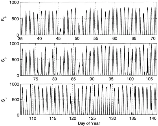
bud-getmeter and a Skey located at 2 m above the ground. Soil moisture, temperatures, and ground heat flux sensors were identical to B123's. The climatic parameters were measured once for both parcels as the two parcels were close from each other. The air temperature was monitored at 6 m high by Vaisala HMP45C probes, and the shortwave incoming radiation was recorded by a 3 m high CM5 pyranometer.The solar incoming radiation measured from DOY 35 to DOY 145 is shown on Fig-ure B-2. Only few cloudy days are present during the whole period of measFig-urements.
Cloudy conditions lead to a drop in solar incoming radiation and are therefore easy to determine compared to sunny days. The daily maximum value of solar incoming radiation is generally high, even in the mid-Winter maximum values of 700 W.m-2 are common. In the late April, the solar incoming radiation can generally reach 900 to 1000 W.m-2
at solar noon. Air temperature was recorded for the same period. As seen on Figure B-3, the range of air temperature is pretty large, with minimum temperature of about 2 'C at night in January, and maximum temperatures of about 40 'C in late April. Air specific humidity is generally low, as seen on Figure B-4. Indeed the relative humidity in the air is relatively small in this semi-arid region. Even when air temperature rises to 40 0C in late April, the specific humidity rarely exceeds 10 gH2o/kgzr. Wind speed was measured at 2m height. The wind speed cycle is shown on Figure B-3. Wind speed fluctuates faster than the other environ-mental variables and was generally below 5 m.s 1. Net radiation was recorded at 2m above the ground, and usually reached a maximum of 400 W.m 2 in February to almost 750 W.m-2
in late April just before harvest. Some sensible and latent heat flux data was missing due to the sensor sensitivity to bad weather conditions, in particular after a strong rainfall event. Sensible heat flux was small at the begin-ning of the measurement period with a maximum value of about 100 W.m-2, and became really high during the senescence period leading to daily maxima of the order of 250 W.m-2. Latent heat flux was also pretty low at first, when the vegetation was growing and installing, but it became very large just before the senescence period, reaching high values of the order of 400 W.m-2. The ground heat flux was calculated as the mean value of the 3 measuring plates. This mean value is seen on Figure B-9. The maximum possible values reached 150 W.m 2 just after sowing, when there was almost no vegetation shade. The smallest amplitude of the flux was obtained before senescence, when the vegetation cover and the greenness were high.
1.3
Calibration and validation of the SVAT model
1.3.1
Calibration
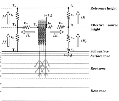
The Soil-Vegetation-Atmospher-Transfer (SVAT) model is named ICARE SVAT and it is described in the article submitted to Agricultural and Forest Meteorology. This model describes the evolution of the soil water content and temperature profiles using the energy budget over the soil and canopy. Because the SVAT model requires a significant number of parameters, we first performed a sensitivity analysis in order to identify the importance of each parameter for calibration. We first used a priori values taken from both literature review and field measurements. The parameters calculated using field measurements or empirical models related to the soil composition are: the soil hydraulic conductivity at saturation ksat, the shape parameter of Brooks and Corey retention curve B, the soil water content at field capacity Ofc, the soil
water content at wilting point 9
,ilt, and the water content at saturation sat. The
parameters derived from literature review are the soil resistance parameters Ars8,
Brss, and the stress parameters of the stomatal resistance Dp, DT and the minimum
stomatal resistance rsc,min. The calibration of the model was based on an iterative procedure, which compared the time series of estimated variables (Yest) and observed variables (Yobs) and minimized their difference by adjusting the chosen parameters. The optimization was obtained by minimizing the Root-Mean-Square Error (RMSE) between the two time series.
F
N 1/2RMSE N 1 I Yob,(1) - Yst2
n=1.
with N: number of observations. The initial values of the parameters are the a priori values. The minimization treated the parameters following their importance, found after the sensitivity test. The optimization iteratively used the simplex search method on Matlab (The Mathworks Inc.).
1.3.2
R3 site
Samples of the soil were analyzed to determine the fractions of clay and sand. On R3-B123, 47.5 % of the soil was clay and 15.8 % was sand. On R3-B130, 36 % of the soil was clay and 16 % was sand. Then using gravimetry tests, Brooks and Corey 1964 retention curves were fitted to the data. On R3-B123, we obtained for the potential at saturation 4
'sat = -0.3 m and the shape parameter of the curve B = 5.25. Then the
following values were found: soil water content at saturation wsat = 0.47 m3 .M
soil water content at field capacity wfc = 0.37 m3.m-3 and soil water content at
wilting point wilt = 0.14 m3.m-3. On R3-B130, the following values were found:
=sat -0.135 m, B = 4.5, Wsat =0.46 r 3.m-3, wfc = 0.30 m3.m 3 and wil =
0.09 m3.m-3. The soil hydraulic and thermal properties were also measured in situ.
The following values were found on R3-B123: the soil dry density was 1.55 kg.m-3,
the soil specific heat was 900 J.(kg.K)-1 and the dry thermal conductivity:
Adry =
0.03 W/(K.m) and the hydraulic conductivity at saturation ksat =1.25 * 10- m/s.
Then the SVAT parameters that could not be directly measured were calibrated to fit the measured fluxes and observed radiative temperatures at 0' and at 55'. In particular, the parameters of the soil resistance to evaporation, were calibrated at the beginning of the measurements when the wheat was very short. The following coefficients were found A,, = 11. and Brs, = 11. . The roughness length of the substrate was found to be zo,, = 0.03 m.
After installation of the canopy, the calibration of the vegetation parameters was done. The minimum stomatal resistance was found to be: rsc,min = 90 m.s 1, the
water vapor deficit stress factor parameter of the Jarvis formulation: Dp = 1.5e -4 Pa-1 , and the temperature stress factor parameter DT = 0.004 K-. All those parameters were calibrated on R3-B123 in 2003 and validated on R3-B130 during the same period. The best set of parameters matching both the calibration and validation were chosen.
1.3.3
Agdal site
The approach to calibration and validation of the parameters over Agdal is different than for the R3 site. At Agdal we had flux measurements for more than six months. Therefore, the parameters were calibrated on the first three months of measurements and validated on the second half. The soil thermal and hydraulic properties were found to be: soil composed of 20 % of clay and 56 % of sand, the potential at sat-uration V/'sat = -0.703 m, the shape parameter of the Brooks and Corey retention curve B = 6., soil water content at saturation 0
,at = 0.38 m3.m 3, soil water con-tent at field capacity Of, = 0.23 m3.m 3 and soil water content at wilting point
0
wilt = 0.08 m3 . m-3 , the soil dry density was 1.44 kg.m-3, the soil specific heat was 840 J.(kg.K)-' and the dry thermal conductivity: Adry = 0.03 W.(K.m)-1 and the hydraulic conductivity at saturation ksat = 2.7 * 106 m.s1 .
The following evaporation and transpiration parameters were found: Ars,
-11.75 and Brs = 12.27 , zo,, = 8*10-3 m, rsc,min = 150 m.s1 , Dp = 2.5e-4 Pa-I
Chapter 2
Frequency analysis of EF
2.1
Frequency analysis of EF
2.1.1
Fast Fourier Transform (FFT)
To understand the diurnal behavior of EF, EF was first computed using the measured turbulent fluxes: the sensible heat flux H and the latent heat flux AE as:
EF =
AE
H +AE
However as we can see on figures B-7 and B-8, some of the flux data was missing, therefore a FFT could not be computed as it requires continuous data, separated by the same interval of time.
2.1.2
Fast Fourier Transform (FFT) on moving window
To solve this problem, the first idea was to use a FFT on each window of non-missing data and then the resulting FFTs, weighted according to the energy of the window, to conserve energy. However, this method could not lead to satisfying results. Generally, the windows of non-missing data do not have the same length, leading to different Fourier base frequency. The resolution of the flux data set remains the same
the minimum Fourier frequency is: WF = . All other frequencies are proportional to this frequency, so our set of Fourier frequencies is w, = n.WF = 2. Therefore, the set of Fourier frequency is changing for each different window. This leads to a strong biases in the spectrum of EF. The spectrum cannot permit a satisfactory interpretation of EF diurnal behavior.
2.1.3
Lomb periodogram
The third approach was to use the Lomb periodogram approach as described in Van
Dongen 1999 [55], Laguna 1998 [52] and Lomb 1976 [53]. This method allows a
frequency analysis of unevenly spaced data. It was first developed for the frequency analysis of astrophysical data, that were available at different times, not necessary evenly spaced in time. This method is based on Discrete Fourier Transform (DFT) for unevenly sampled signal, x(t,), n = 1, 2, .. , N:
N
DFT(w) = x(t)ew'
n=1
with w = 27rv: angular frequency. This can be used to define the Lomb periodogram,
which is not dependent on the initial time considered, like the commonly used peri-odogram.
N 2 N2
C
1
[zn=1
x(tn)coS [w(t, -
T(w))]][ZnL
1
X(tn)Sir [W(t-r(w))]
P(w ) =
22Z
jN cos2 [w(t7_ - T(W))] N sin2 _W) ]Where o2 is the variance of x(tn) and:
1
EN_____r(w) = -Arctan n=
2w k N_ cos(2wtn)
is an offset to achieve time translation invariance of the periodogram. The main idea of the Lomb periodogram is to fit a sinusoidal function of frequency w to the
components of EF, using the measured turbulent heat fluxes. For instance, when trying to reconstruct the initial turbulent fluxes, using this method we obtained a very noisy resulting signal as seen on figures B-10 and B-11. This proves that the periodogram was not able to correctly determine the frequencies of interest in the fluxes. Indeed, the fluxes are very different from one day to another because of the varying environmental factors such as the solar incoming radiation, air temperature or wind speed. It is also clear that the frequency behavior of the environmental parameters is very complex because of the inherent variability of the environmental conditions.
Chapter 3
Analysis of EF diurnal behavior
3.1
Article submitted to Agricultural and Forest
Meteorology
The following article was submitted to Agricultural and Forest Meteorology. This article describes the mean diurnal cycle of EF, depending on the different environ-mental and soil moisture conditions. Added discussions and plots, which could not fit into the paper required length are presented here after the article.
Analysis of Evaporative Fraction Diurnal Behavior
Pierre Gentine and Dara Entekhabi (Correspondent author) gentinea~mit.edu and darae(dimit.edu
Department of Civil & Environmental Engineering Massachusetts Institute of Technology (MIT)
Cambridge, Massachusetts
USA 02139
Abdelghani Chehbouni, Gilles Boulet and Benoit Duchemin
ghaniAdcesbio.cnes.fr, Gilles.Boulet( cesbio.cnes.fr and benoit.duchemin(d1cesbio.cnes.fr Centre d'Etudes Spatiales de la Biosphere (CESBIO)
18 Avenue Edouard Belin
BPI 2801
31401 Toulouse CEDEX 9 France
Submitted to Agricultural and Forest Meteorology April 7, 2006
Abstract
Experimental studies indicate that Evaporative Fraction (EF), the ratio between the latent heat flux and the available energy at the land surface, is a normalized diagnostic that is nearly constant during daytime under fair weather conditions (so-called daytime self-preservation). This study examines this indication and investigates contributions to the variability of EF due to both the environmental factors (air temperature, solar incoming radiation, wind velocity, soil water content or Leaf Area Index) and due to the natural phase shift between the surface energy balance components at the land surface. It is shown that the phase difference between soil heat flux and net radiation needs to be characterized fully for application of EF daytime self-preservation. The correlation of EF with the different environmental factors is then discussed. Finally the conditions under which the diurnally-constant EF assumption can be invoked are discussed. In the last part of the study, the effect of non-precipitating partial cloud cover on EF and evapotranspiration are analyzed. This latter test is important to extension of the EF measure to non-fair weather conditions.
1. Introduction and Motivation
Evapotranspiration (ET) is a flux linking water, energy and carbon cycles. Flux measurement networks (as FluxNet, EuroFlux, AmeriFlux) are only available in few tens of point locations around the Globe. They are costly both to install and maintain. Moreover there is a strong heterogeneity of the fluxes over the land surface because of the inherent physical diversity of the land and vegetation properties with wide range of length scale. Therefore the locally-measured fluxes cannot be representative of a whole region of interest.
The only currently available way to obtain ET mapping is to rely on remote sensing data that now have both nearly-continuous spatial coverage and adequate temporal sampling using constellation of satellites or geostationary platforms. It is not possible to directly measure fluxes using satellite information. In fact the remotely sensed measurements such as land surface temperature are only indirectly related to the state of the land surface and the corresponding heat fluxes.
Different methods have been developed to estimate ET using either empirical or physically based methods (see Capparrini et al. (2004) for review). In summary there are four main approaches:
1. The first approach is to use remote sensing data such as Normalized Difference Vegetation Index (NDVI) and Land Surface Temperature (LST) and to empirically link those variables to surface evapotranspiration, as in Gillies et al.
(1997) and Moran et al. (1994). This approach is limited to locations where
calibration and validation data are available. Extensions beyond the calibration region and the studied climate have unknown errors.
2. The second approach is based on using the LST and NDVI images to constrain the energy budget at the land surface. In this approach, the ground heat flux G is usually related to another flux such as the surface net radiation Rn, which can be more easily estimated from remote sensing. Several empirical relationships have been used, such as: G/Rn = const. and G/R, =
f
(ND VI), as in ALEXI model; see Anderson et al. (1997), Mecikalski et al. (1999) or G /R =f
(NDVI,LST), assoil heat flux cannot be simply related to the net radiation and depends on
different factors that cannot be directly measured, in particular the soil moisture
profile. Furthermore, the effect of solar angle (e.g Ma et al. 2002) and the time lag
between G and R, have to be accounted. In fact there are large phase differences
between the two that can lead to serious errors in turbulent flux estimation based
on the land surface energy budget.
3. The third approach uses the assimilation of remote sensing data into Soil
Vegetation Atmosphere Transfer (SVAT) models, as described in Dunne and
Entekhabi (2006), Pellenq and Boulet (2004) and Reichle et al. (2002). The ET at
the land surface is physically constrained by the SVAT model whose state and
intrinsic parameters are calibrated to fit the remotely sensed observations such as
LST. Where micrometeorological measurements are continuously available, the
water and temperature state of the model may be solved using the coupled
hydraulic and energy budgets at the land-surface. Hence, ET time-series may
hence be calculated at the time-step of the model.
4. The fourth approach has been introduced by Castelli et al. (1999) and Boni et al.
(2000 and 2001) and extended by Capparrini et al. (2003 and 2004). It is based on
a variational assimilation of LST into a surface energy balance model. In this
approach there is no direct use of the water budget, but only of the energy budget
at the land surface. The most interesting part of this approach is that it does not
require any empirical relation linking ET to the remotely sensed data, and it also
does not require any empirical relationship assumption between soil heat flux and
net radiation. The main idea of this approach is to estimate the most sensitive
parameters of flux estimation using sequences of satellite-based LST imagery.
The first group of parameters is related to the influence of land surface
characteristics on near-surface air turbulent conductivity, namely the roughness
length scale for turbulent heat flux. The time changes in this parameter depending
mainly on the phenological state of the vegetation (assumed to be monthly
constant). The second group of parameters is related to the partitioning of the
turbulent heat fluxes between sensible and latent heat flux. This partitioning is
characterized by the daytime-EF that is linked to the soil moisture conditions.
The second and fourth approaches often rely on the daytime self-preservation of
evaporative fraction EF, which is defined as the ratio between the latent heat flux and the
available energy at the land surface EF
=
,
or a similar diagnostic of the surface
R, -G
energy balance. The robustness of this assumption and the range of its applicability
under different environmental conditions is the rationale for this study.
The observation that EF is often constant during the daytime is based on
Shuttleworth et al. (1989), Nichols and Cuenca (1993), Crago (1996a) and Crago and
Brutsaert (1996). They use in situ measurements of surface energy balance components
to show that EF is almost constant during the daytime hours under clear skies. EF
supposedly removes available energy diurnal cycle and isolates surface control (soil and
plant resistance to moisture loss) on turbulent heat flux partitioning. These controls vary
on approximately daily time-scales.
In an important study Lhomme (1999) has shown that EF is not really constant
during day-time especially in non-fair weather conditions. This leads to ET estimation
errors, in particular in the morning and late afternoon due to the typical parabolical shape
of EF. Lhomme (1999) is the foundation for this study and the analysis here is intended
to provide additional detail. Lhomme (1999) and this study together should provide the
basis to understand the daytime self-preservation of EF and assess the limitations of its
application.
In order to better understand the diurnal behavior of EF and its environmental
dependencies it is important to have long term field experiment data. In this paper we
use a SVAT model in conjunction with field experimental data in order to assess the EF
temporal behavior under diverse environmental conditions. The dual-source (soil and
vegetation) SVAT model also allows the test of the influences of vegetation cover and
soil moisture on EF daytime self-preservation. This model is also used to understand the
possible phase shift between the different surface fluxes, which can lead to dramatic EF
under/overestimation.
The field experiment data used in this study is first presented. The SVAT model
outlined in Figure 1 is described in the Appendix. Then, the diurnal course of EF is
physically explained through SVAT modeling and its consistency with Lhomme's (1999)
result is discussed. The partial soil moisture and vegetation cover influences on the EF
diurnal shape is further analysed. Finally, the temporal correlations between EF and the
main environmental factors are discussed and a strategy for the refinement of ET
estimation using both land surface temperature and EF daytime self-preservation is
forwarded.
2. Field Experiment Data Set
The SVAT model (see Appendix A) is calibrated and tested on two wheat parcels
and one olive tree orchard during the 2002 and 2003 SUDMED project in the region of
Marrakech, Morocco, described in further detail in Duchemin et al. (2006). The
experiment area is a typical Mediterranean semi-arid region. This region is heterogeneous
in terms of vegetation cover and climate both spatially and temporally. These conditions
are particularly appropriate to test and apply SVAT models because of the sparse
vegetation with strong phonological cycle permits variations in the contribution of soil
and vegetation to the surface energy balance. The air temperature ranges from as low as
0
0C in the Winter to 50'C in the Summer; LAI from 0 (sowing) to more than 5 before
harvest.
The study site is composed of sparse vegetation (varies with season) in which
latent and sensible heat fluxes are of comparable magnitude. There are both bare soil and
canopy contributions to turbulent fluxes. The specific study site, named R3, is located in
an irrigated area in the Haouz plain surrounding Marrakech, where wheat is the main
cultivated plant.
The R3 site is a 2800 ha area where irrigated wheat is cultivated, located 45 km
East of Marrakech. Two fields were equipped with instrumentation, namely the 123rd
(R3-B123 used in this study) and 130th (R3-B130) parcels. The parcels are cultivated
with wheat. The sowing date is January 13 (Day Of Year 13). The climate is
characterised by a dry and warm period with very few precipitations events in Summer
and Fall. Almost all of the annual precipitation occurs in Winter and Spring (see Fig. 2).
The rainy period lasts 6 months from November to April and the cumulative precipitation
is generally of the order of 250 mm per year. The site is periodically irrigated by flooding
the entire field. The parcel of interest in this study is r#-B123. Irrigation events occurred
on February 4th (DOY 35), March 20th (DOY 79), April 13th (DOY 103) and April
2 1th(DOY 111) with a mean 25 mm supply each time (see 2).
Energy fluxes were continuously monitored starting February
4th(DOY 35) and
lasted the entire wheat season until May
2 1s'(DOY 141). It covered the whole wheat
cycle: sowing, vegetative growth, full, canopy, and the senescence. Vegetation appears
around February 7 (DOY 38), with a growth peak on April 20 (DOY 110), followed by
the senescence period until the end of May (see Fig. 3).
Near-continuous measurements have been recorded during the entire wheat
season. Sensible heat flux was measured with a 3D sonic anemometer (CSAT3, Campbell
Scientific, Logan, UT) at 3m height. A KH20 krypton hygrometer also measured the
latent heat flux at this height. The soil heat flux is monitored by three heat flux plates at 1
cm below the surface, 2 plates at 10 cm and 1 plate located at 30 cm. The net radiation is
monitored by a CNR1 located at 2 m above the ground. Moisture is monitored by several
Time Domain Reflectometry (TDRs) located at 5, 10, 20, 30, 40, 50 cm below the surface
and soil temperatures are measured by some thermistances located at the same distance
from the soil surface. Flux values derived from measurements that were obviously either
too high or too low have been replaced by time-interpolated values, and when several
errors occurred during one entire day, the flux data for that day was rejected.
The air temperature was monitored at 6 m height using Vaisala HMP45C probes,
and the shortwave incoming radiation was recorded by a 3 m height with a CM5
pyranometer.
The meteorological conditions are highly variable. Solar incoming radiation
varies between a diurnal maximum of 200 W.m- for a February cloudy day to a diurnal
maximum between 900 and 1000 W.m- at the end of May (see Fig. 4). There is also a
wide range of air temperatures with a minimum of
00C in February and a maximum of
38'C by the end of May.
The average energy balance closure between the measured turbulent heat fluxes
H
+ IE and the measured available energy
R -G is 79% and they have 89% explained
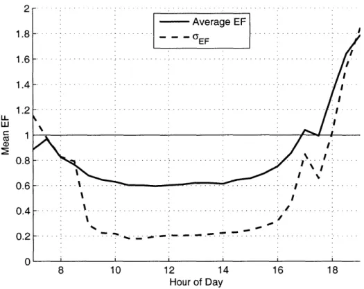
Past experimental EF studies were only able to study the EF behaviour during a
few days because continuous experimental flux data are both complicated and costly to
maintain. The R3-B123 meteorological and flux dataset offer measurements for more
than 100 days. Fig.
5
shows the daily course of EF using the measured latent and sensible
heat fluxes averaged over the DAY 35 to DAY 141. EF exhibits a typical concave-up
shape with a minimum around 12PM (all times are referenced to local solar conditions so
12PM is local solar noon). The EF values are nearly constant during mid-day period.
Near sunrise or sunset EF and its standard deviation increase sharply. Available energy
that appears in the denominator of EF is small near these times. Therefore the inclusion
of early morning and late afternoon EF values in the estimation of daily EF can lead to
non-negligible evapotranspiration estimation errors. The EF behaviour in those periods
will clearly depend on environmental factors, soil water content, and phenological stage
as well. Some of these influences were investigated in Lhomme (1999) through SVAT
modelling. This study builds on the same approach but extends it in important ways.
Specifically the contributions of soil and vegetation and the phase shifts between the
energy balance components are the subject of analyses. Application with the
extended-duration field observation data allows for realistic experimental conditions.
3. Lhomme (1999) Study
Lhomme (1999) analysed the daytime pattern of EF using the Penman-Monteith
single-source model coupled to a convective boundary layer model. The influence of both
the micrometeorological factors and soil water availability on the EF daily course was
investigated in this article. Lhomme (1999) found that EF exhibits a typical concave-up
shape, with a minimum around noon. Moreover EF appeared to be relatively constant
around mid-day yet always lower than the mean daily value. The soil moisture
availability was found to have a great importance on EF, and that EF was a strongly
increasing function of soil water content, for high incoming radiation and wind speed
values. When available energy is not limiting the EF amplitude is directly related to soil
water availability. EF was also found to decrease when solar energy is increased for
medium soil water conditions and high wind speed. Lhomme (1999) also found that the
air vapor saturation deficit only had a slight impact on EF amplitude and that wind
velocity had almost no effect on EF.
However in his approach Lhomme (1999) assumed that the soil heat flux was a
fraction of the net radiation energy. Hence the soil heat flux (G) and net radiation (Rn)
were forced to be in phase. This can lead to large biases in the available energy (Rn-G)
diurnal behaviour. Moreover G is generally negative in the mid-afternoon, leading to a
much smaller EF.
4. Phase Difference Between G and Rn
Many previous studies have shown that the phase difference between soil heat
flux and net radiation is an important characteristic of surface energy balance (Fuchs and
Hadas 1972; Idso et al. 1975; Santanello and Friedl 2003). The difference between these
two fluxes appears in the denominator of EF. In fact it is the normalization of latent heat
flux diurnal cycle by the diurnal cycle of this difference that is key to the apparent
daytime self-preservation of EF.
Usually EF exhibits a typical concave-up shape with a minimum in the early
afternoon (See Fig 5). Few studies have tried to theoretically explain the EF shape.
Among those studies Crago (1996b) and Lhomme (1999) explained the diurnal shape
using a single-source Penman-Monteith formulation for ET since they focused on
closed-canopy vegetation. In those studies, the soil heat flux was considered either negligible or
a constant small fraction of the net radiation. However, some studies (Clothier et al.
(1986), Kustas et al. (1990)) have shown that the soil heat flux can be an important part
of the energy budget and expressing it as a fraction of the incoming radiation does not
represent the physics of conduction. Indeed, soil heat flux is dependent on many factors
such as vegetation cover, soil type and moisture or time of day. In particular, Fuchs and
Hadas (1972), Idso et al. (1975) and Santanello and Friedl (2003) found important phase
difference between G and Rn around solar noon.
When G is expressed as a fraction of the net radiation it is usually underestimating
the real soil heat flux in the morning, and overestimation in the afternoon, leading to a
Hence G is an important component of the surface energy budget and is also of drastic
importance to understand and explain the EF diurnal shape.
In Fig. 6 and 7 the long duration SUDMED field experiment data and the SVAT
model are used to estimate the fidelity of the in-phase G and Rn assumption. The SVAT
model was run for different soil moisture, LAI and environmental conditions allowing the
calculation of the constant fraction relating G and Rn with:
f sunsetGtdJG(tjdt
S
sunrise (1)f unset
f'sR, (t)dt Jsunrise Rtd
The LAI and soil moisture were fixed but varied over a range in order to assess
the role of surface water limitation and fractional vegetation-versus-soil energy balance
contributions. Three LAI values (0.5, 2.5 and 4.5) were used to find the average value of
f over the entire period with many soil moisture conditions. Soil moisture is specified for
the top 5 cm and the profile is allowed to reach hydrostatic equilibrium. The mean values
found were f=O.14 for LAI=0.5, f=O.1 1 for LAI=2.5. f=O.09 for LAI=4.5 using (1).
Figure 6 shows the difference between the SVAT modelled soil heat flux and the
soil heat flux calculated as a fraction of the net radiation. The difference is negative
during most of the day except in the morning, usually from 8AM to 12.30PM. When G is
expressed as a fixed fraction of the incoming radiation (hence in phase), it is
underestimating the soil heat flux in the morning and overestimating during the rest of the
day in particular in the afternoon where the absolute difference can become large.
Moreover, the difference is strongly depending on LAI: it is clearly increasing in sparse
canopy cases, as the amplitude of both soil heat fluxes is increasing due to the increasing
fraction of radiation reaching the ground. The difference is lightly dependent on soil
moisture; with high soil moisture the surface thermal gradient is smaller because of the
larger thermal inertia of the water within the porous medium. Even if the wet thermal
conductivity is higher, the wet surface thermal gradient is so small that the surface soil
heat flux is smaller in a wet case than a dry case in the morning. In the late afternoon,
when the soil heat flux is becoming negative, the amplitude is still larger in the dry case
because of the same surface thermal inertia effect. Fig. 6 shows that the two fluxes are
always out of phase. This can be seen more succinctly in Fig. 7 where the difference between the two are shown.
In Fig. 7 the soil heat flux error is generally maximum in the mid morning, for all
LAI and soil moisture conditions. It becomes negative in the mid afternoon essentially
cancelling the net radiation at that time. This strong asymmetry in the errors of the in-phase assumption will have an effect on the diurnal shape of EF. In particular, the EF shape is less parabolic than the one found by Lhomme (1999). Indeed the larger soil heat flux at the early daytime hours will sharpen the EF shape at the beginning of the day. Then as G is smaller and even negative in the afternoon, EF does not increase as rapidly as in the in-phase case. The increase will be present as long as the soil water content is not high because the presence of liquid water decreases the amplitude of the soil heat
flux.
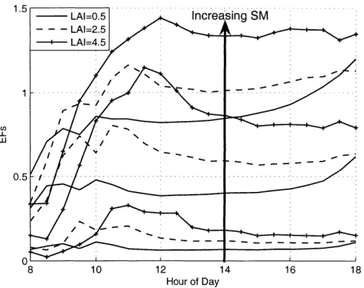
5. EF Diurnal Pattern Dependencies
The instantaneous Evaporative Fraction is defined for total, soil, and canopy as (respectively): EF(t) =
E(t)
(2) Rn(t) - G(t) 2E (t) EF, (t)= AE't (3) Rn, (t) -G(t) E,()AE 0(t)(4 EFe(t)= ' (4) Rn'(t)The degree of their convexity during the day (hence the violation of daytime self-preservation) is sensitive to the soil water control on evaporation as well as the sparsity of the canopy. The degree of dependence can be shown through SVAT modelling calibrated and forced with SUDMED observations and micrometeorological forcing. The two critical factors, soil moisture and LAI, are varied in order to quantitatively assess the effects. Figure 8 shows the diurnal behaviour of total EF under the different soil moisture and canopy cover conditions. The instantaneous EF values are averaged over the whole measurement period using (2). In every case EF exhibits a convex diurnal shape as found


![Fig. 18: Relative cumulative evapotranspiration error [%*100] from DAY 35 to DAY 141 using the daily mean EF value, for LAI equals to 0.5, 1.5, 2.5, 3.5 and 4.5.](https://thumb-eu.123doks.com/thumbv2/123doknet/14175927.475335/69.918.158.694.145.559/relative-cumulative-evapotranspiration-error-using-daily-value-equals.webp)