Adapting rain data for hygrothermal models

Publisher’s version / Version de l'éditeur:

Building and environment, 44, 5, pp. 987-996, 2008-08-09

READ THESE TERMS AND CONDITIONS CAREFULLY BEFORE USING THIS WEBSITE.

https://nrc-publications.canada.ca/eng/copyright

Vous avez des questions? Nous pouvons vous aider. Pour communiquer directement avec un auteur, consultez la

première page de la revue dans laquelle son article a été publié afin de trouver ses coordonnées. Si vous n’arrivez pas à les repérer, communiquez avec nous à PublicationsArchive-ArchivesPublications@nrc-cnrc.gc.ca.

Questions? Contact the NRC Publications Archive team at

PublicationsArchive-ArchivesPublications@nrc-cnrc.gc.ca. If you wish to email the authors directly, please see the first page of the publication for their contact information.

Archives des publications du CNRC

This publication could be one of several versions: author’s original, accepted manuscript or the publisher’s version. / La version de cette publication peut être l’une des suivantes : la version prépublication de l’auteur, la version acceptée du manuscrit ou la version de l’éditeur.

For the publisher’s version, please access the DOI link below./ Pour consulter la version de l’éditeur, utilisez le lien DOI ci-dessous.

https://doi.org/10.1016/j.buildenv.2008.07.002

Access and use of this website and the material on it are subject to the Terms and Conditions set forth at

Adapting rain data for hygrothermal models

Cornick, S. M.; Dalgliesh, A.

https://publications-cnrc.canada.ca/fra/droits

L’accès à ce site Web et l’utilisation de son contenu sont assujettis aux conditions présentées dans le site LISEZ CES CONDITIONS ATTENTIVEMENT AVANT D’UTILISER CE SITE WEB.

NRC Publications Record / Notice d'Archives des publications de CNRC:

https://nrc-publications.canada.ca/eng/view/object/?id=816e505a-5971-4302-9b29-bc21f0e23f53 https://publications-cnrc.canada.ca/fra/voir/objet/?id=816e505a-5971-4302-9b29-bc21f0e23f53

A d a p t i n g r a i n d a t a f o r h y g r o t h e r m a l m o d e l i n g

N R C C - 5 0 8 3 2

C o r n i c k , S . M . ; D a l g l i e s h , A .

2008-10-01

A version of this document is published in / Une version de ce document se trouve dans:

Building and environment, v. 30, 2008

The material in this document is covered by the provisions of the Copyright Act, by Canadian laws, policies, regulations and international agreements. Such provisions serve to identify the information source and, in specific instances, to prohibit reproduction of materials without written permission. For more information visit http://laws.justice.gc.ca/en/showtdm/cs/C-42

Les renseignements dans ce document sont protégés par la Loi sur le droit d'auteur, par les lois, les politiques et les règlements du Canada et des accords internationaux. Ces dispositions permettent d'identifier la source de l'information et, dans certains cas, d'interdire la copie de documents sans permission écrite. Pour obtenir de plus amples renseignements : http://lois.justice.gc.ca/fr/showtdm/cs/C-42

Adapting Rain Data for Hygrothermal Models

Steve Cornick1 * _{and W. Alan Dalgliesh}2

Abstract

Design for moisture control has now become an established part of building envelope design. Hygrothermal modeling tools, capable of simulating moisture transfer in materials, are a key element of the design process. There are three principle methods of moisture transfer in envelopes. They are, in order of magnitude, capillary action, vapour convection, and vapour diffusion. Wind-driven rain has the potential to deposit large amounts of liquid water on the exterior surface, as well inside walls through rain penetration, providing a significant source for moisture transport. Most hygrothermal models are capable of handling wind-driven rain impinging on or penetrating the surface of the envelope. Correct results presuppose the availability of reliable rain intensity data. Many data sets however do not record hourly rain intensities but qualitative intensities such as light, moderate, or heavy. This paper examines several methods for assigning quantitative values to weather observations available in Canada. Real data, such as data from rain gauges , is preferable although the latter have shortcomings. Differences in catch can be up to 50% depending on gauge type, size, and exposure. When only rain codes are available the values recommended by the local meteorological service can provide adequate estimates. In case where there is observer bias a better estimate can be obtained by adjusting the value for light rainfall. If very little information is available stochastic modeling of rainfall is possible though the accuracy, especially for individual months is low.

Keywords

Hygrothermal-simulation, Modeling, Moisture, Building envelope, Wind-driven rain, Climate, Stochastic-modeling.

Nomenclature

Greek symbols Latin symbols

β Shape parameter T Random variate

γ Location parameter MBE Mean Bias Error

η Scale parameter RMSE Root mean squared error

Latin symbols a, b Regression parameters

H Intensity of heavy rainfall,

mm/h rain Mean annual rainfall, mm

L Intensity of light rainfall,

mm/h· rainydays Mean annual number of days with rainfall > 0.2mm

M Intensity of moderate

rainfall, mm/h·

Introduction

The design and management of building envelopes have become increasingly sophisticated. Assessment of the performance of proposed and existing designs is now being done through computer simulations [1, 2]. Maintenance management systems now use computer models to assess a range of maintenance options [3, 4]. Examples of a typical computer simulation commonly used are hygrothermal models. Hygrothermal models simulate the heat, air, and moisture transport processes through materials [5, 6, 7, 8, 9, 10, 11]. These models are commonly used to assess the moisture management capabilities of portions of building envelopes. Many examples exist in the literature including but not limited to retrofit studies [12], drying

1 _{National Research Council of Canada, Institute for Research in Construction Building M-24, Montreal}

Road Campus, 1200 Montreal Rd., Ottawa, Ontario, Canada. K1A 0R6, Facsimile: +1 613 998 6802 Email: steve.cornick@nrc.ca

* _{Corresponding author}

studies [13, 14], and performance assessments of envelope systems, some verified with experimental data [15, 16, 17, 18, 19]. Hygrothermal models also form the basis for other models providing input for damage models of corrosion, mould, and rot [20, 21]. The area of whole building performance takes a holistic approach to building performance coupling hygrothermal models with energy, airflow simulations, and computational fluid dynamics models of the building exterior [22, 23, 24, 25, 26, 27]. Given the prevalence and important of hygrothermal modeling it is necessary that uncertainty in the input data, especially with regards to the weather data, be recognized. Generally hygrothermal models require a significant input in the form of actual weather data or some specified reference year [28, 29, 30]. The quality and availability of weather data are increasing yearly. There is however a difficulty; hygrothermal models generally require a quantitative measure for rainfall. In fact the availability of rain in the weather input is key to proposed methodologies for assessing envelope performance [31, 2]. These methodologies assume wind-driven rain impinges on building facades and that certain amounts of liquid water penetrate the exterior cladding. In order to calculate the amount of wind-driven rain hourly rainfall intensities and coincident wind speed and direction are required [32, 33, 34]. Therefore reliable rain data is required in weather data sets for building applications. While many datasets, such as SAMSON [35] and HUSWO [36] include hourly rain totals other datasets such as the CWEEDS [37] include only qualitative data. In addition to the weather sites that comprise datasets such as SAMSON, HUSWO, and CWEEDS there are many stations that report data that, although not up to the World Meteorological Stations standard for weather stations, nevertheless include enough data that could be used for modeling purposes. Most of these stations however only record qualitative rain data.

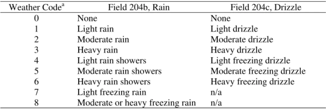
The CWEEDS datasets are stored in WYEC2 format [38]. In this format there is no column for hourly precipitation. Precipitation is recorded as one of nine single digit codes. Two of these codes describe the occurrence of rain and drizzle. Field 204b represents the occurrence of rain, rain showers or freezing rain. Field 204c represents the occurrence of drizzle or freezing drizzle. The codes and the corresponding meanings are given in Table 1. There are also guidelines for the observer as to the assignment of codes. These guidelines were published by Environment Canada [39, 40]. Solid forms of precipitation such as hail and snow, which are stored in other columns of the observations field, were not considered. Increasingly the recording of present weather and weather data is being automated. In some cases, depending on how the precipitation was measured (an observer, a tipping bucket, or radar gun), there might be real rain data for a CWEEDS site. However, Canadian automated stations, such as Automated Weather Observation System (AWOS) still report in the same format. Consequently quantitative rain data is reported in the CWEEDS files as an observer code but is stored separately where available. CWEEDS data was obtained from Environment Canada as was tipping bucket rain data from the digital archive of Canadian climatological data [37]. For the tipping bucket data 27 stations, mostly data from airport stations, were obtained with periods ranging from 4 to 43 years. The guidelines for rainfall intensities are given in Table 2.

TABLE 1 — Present weather codes for precipitation in the CWEEDS dataset

Weather Codea _{Field 204b, Rain Field 204c, Drizzle}

0 None None

1 Light rain Light drizzle

2 Moderate rain Moderate drizzle

3 Heavy rain Heavy drizzle

4 Light rain showers Light freezing drizzle

5 Moderate rain showers Moderate freezing drizzle

6 Heavy rain showers Heavy freezing drizzle

7 Light freezing rain n/a

8 Moderate or heavy freezing rain n/a

a_{If several phenomena occur simultaneously, the highest WYEC2 value is reported.}

One is at first tempted to simply substitute the suggested rainfall intensity for the corresponding code. This may be adequate or even a good start. In fact this method, slightly modified, was used in several projects to produce weather files for hygrothermal models [31, 41] and wind-driven rain calculations [42]. While this

method is good at fully populating the data sets, a requirement for most hygrothermal models, there was some concern as to whether the resulting data sets reflect the actual rainfall. Ideally the dataset would contain quantitative data and as Blocken and Carmeliet [43, 44] suggest at 10-min intervals. Reality is somewhat different. First rainfall data is generally sparse. Sumner [45] gives the UK as an example. With more than 5000 rain gauges in service the UK has one of the most dense rain gauge network in the world. The total area of the coverage represents approximately 5 x 10-12_{% of the landmass of the UK [45]. The}

concentration in North America is considerably sparser. Furthermore most of the weather stations reporting weather, and most importantly, concurrent wind and rain were installed for aviation use. For the moment at least, it seems that hygrothermal modellers will have to be content at times with qualitative hourly data. TABLE 2 — Precipitation intensities and typical intensities [39] as well as the divisions used to separate the intensities [40]

Reported precipitation

intensity, mm/h Rain Showers Drizzle Range for Rain or Showers Range for Drizzle

Light 1.8 1.8 0.1 1.1 to 2.5 less than 0.2

Moderate 5.1 5.1 0.3 2.6 to 7.5 0.2 to 0.4

Heavy 13 13 0.8 7.6 or greater 0.5 to 1.0

The objective of this work was to examine various methods for assigning hourly intensity values to qualitative precipitation intensities. The goal was to develop a method for converting the rain codes in the CWEEDS files to quantitative rain amounts. The method was designed to be robust enough for simulated rainfall to be generated automatically for use with other datasets. For the purposes of this paper long-term data is considered to be climate normal data. Climate normal data is calculated using the World

Meteorological Organization standard 30-year period, 1971–2000 being the current period of record. The assigned values should at least match long-term mean rainfall and reproduce as closely as possible the yearly totals. At this stage, agreement with monthly and daily totals may be too much to hope for.

Previous work

Much work has been in the area of correcting or filling in weather data. Most the work has undertaken in the fields of hydrology and agriculture (see Makhuvha et al. [46] and Acock and Pachepsky [47] for example). Most of the building related has been focused on correcting data for energy simulations [48]. Much of the building envelope related work on the relation between rain and hygrothermal performance has concentrated on wind-driven rain studies. Koronthályová and Matiašovský [49, 50] derived a method for generating hourly wind-driven rain course from 6-h rainfall totals. A sensitivity analysis comparing the hygrothermal response of massive masonry walls using hourly wind-driven data and hourly derived from six-hourly totals showed little difference in the response deep inside the wall. Blocken and Carmeliet in many publications have investigated the effect of wind-driven on facades including examining the effect of averaging errors on wind-driven amounts [43, 44, 51, 52]. Most of these studies used hourly or shorter duration rain gauge data, and coincident wind data, generally measured on-site. In this study however hourly information is readily available except that it is qualitative rather than quantitative.

There have been previous attempts at estimating hourly intensity values from weather observations. In the development of CSA Standard A440 hourly intensities were determined from the weather observations and adjusted using available 6-h rainfall totals [53]. Skerlj refined the procedure by separating the liquid and solid forms of precipitation to estimate the hourly precipitation intensity [54]. In preparing weather data for a parametric study of the hygrothermal performance of walls, hourly intensities were estimated from the weather observation codes by adjusting the light intensity value such that the average rainfall was close to the published long-term mean [55, 56, 57]. This method was also used in the creation of a climate database for a publicly available hygrothermal simulation model as well as a maintenance management system project [41, 3].

Hourly rain intensity and wind speeds have been found to underestimate the rain hitting buildings unless combined as weighted averages of more frequently sampled data. Errors for buildings on three continents ranged from 11 to 45%, reduced to less than 5% by weighted averaging [44]. The 10-min raw data recommended as a starting point is not generally available, however, so this observation is reported here only to provide context for discussing the errors encountered when using various methods on currently available data.

Methods

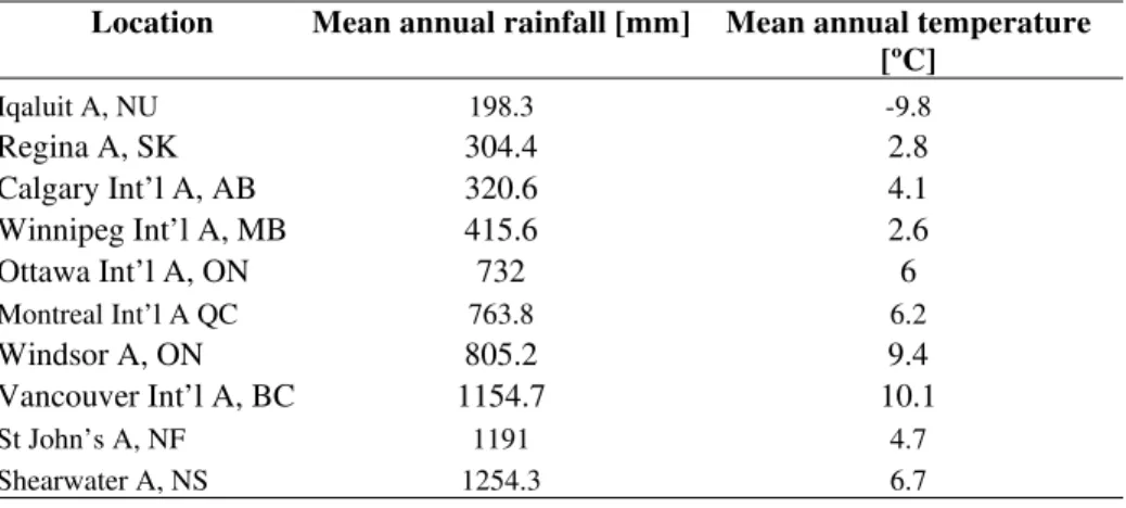
Ten sites with tipping bucket rain data were chosen; Calgary AB, Iqaluit NU, Montreal QC, Ottawa ON, Regina SK, Shearwater NS, St John’s NF, Vancouver BC, Windsor ON, and Winnipeg MB. The climate parameters of interest are given in Table 3. The tipping bucket data was reported hourly and did not include forms of solid precipitation such as hail or snow melt. During occurrences of hail any data reported from the tipping buckets is recorded as missing. These locations are representative of Canada. Each location has at least 8 years of rainfall intensity data [58]. Five different rain files for each location were produced. Only the observations for rain were adjusted. When drizzle was reported the AES codes were used (see Table 2). Five different rain files for each location were created using the following methods.

TABLE 3 — Basic climate parameters for the locations selected for the simulation study. The data shown are climate normal data

Location Mean annual rainfall [mm] Mean annual temperature [ºC] Iqaluit A, NU 198.3 -9.8 Regina A, SK 304.4 2.8 Calgary Int’l A, AB 320.6 4.1 Winnipeg Int’l A, MB 415.6 2.6 Ottawa Int’l A, ON 732 6 Montreal Int’l A QC 763.8 6.2 Windsor A, ON 805.2 9.4 Vancouver Int’l A, BC 1154.7 10.1 St John’s A, NF 1191 4.7 Shearwater A, NS 1254.3 6.7

Method 1: The tipping bucket rain data was used and long-term annual and monthly means were calculated from the tipping bucket data.

Method 2a: Intensity values for light (L), moderate (M), and heavy (H) for rain, showers, and drizzle were taken from those suggested by the local meteorological service [39]. In estimating the amount for showers it was assumed that a rain shower lasted approximately 10 minutes and the intensity values of L, M, and H were reduced accordingly.

Method 2b: Since the bulk of observations and rainfall events, about 95%, occur in the light category adjusting the value L would have the most impact on reducing deviation from the actual rain data. The value for L was constrained by the range recommended by the local meteorological service [40]. M and H were set as above as were the intensity values for drizzle (see Table 2). The value for L was set by adjusting the value such that the Root Mean Squared Error (RMSE) between the estimated amounts and reported long-term values was minimized. For hygrothermal simulations where one of the boundaries is an exterior boundary rainfall is an important parameter, unless the exterior surface is non-absorbent. Rainfall can still be important, however, if wind-driven rain is allowed to penetrate from the exterior through leaks. The sensitivity of building components, such as walls, to moisture damage is largely dependent on the accumulation of moisture over time; therefore it is important to closely match the pattern of rainfall rather than the total rainfall for the year. If the Mean Bias Error (MBE) is minimized the deviations are spread

across the months such that the average error is minimized or zero. This does not produce a rainfall pattern that resembles the long-term pattern. Similarly minimizing the Mean Absolute Error (MAE) may introduce some overall bias in the estimates. By minimizing the RMSE a pattern closer to the long-term rainfall pattern is generated though at the cost of non-minimal MBE and MAE.

Method 2c: Intensity values for drizzle were set as above. L, M, and H were set by adjusting the values such that the RMSE between the estimated annual and monthly means and reported long-term values was minimized. The values for L, M, and H were constrained by the range recommended by the local

meteorological service [40] (see Table 2).

Method 3: This method makes use of a stochastic approach. First for each location a probability distribution for rainfall intensity is determined. The parameters for the distribution are obtained from the tipping bucket data. The three-parameter Weibull probability density function is given in Eq. (1). Drizzle amounts were estimated as in Method 2.

β η γ β

η

γ

η

β

− −⎜⎜_⎝⎛ − ⎟⎟_⎠⎞

⎟⎟

⎠

⎞

⎜⎜

⎝

⎛ −

=

T

e

T

T

f

1

)

(

(1)

0

,

0

)

(

T

≥ T

≥

f

or

γ

,

β

>

0

,

n

>

0

,

−∞

<

γ

<

∞

(2)

Since it is not possible to experience negative rainfall the location parameter, γ, can be set to zero thus reducing the distribution to a two-parameter Weibull distribution, given in Eq. (3). The cumulative density function (CDF) is given in Eq. (4).

β η β

η

η

β

− −⎜⎜_⎝⎛ ⎟⎟_⎠⎞

⎟⎟

⎠

⎞

⎜⎜

⎝

⎛

=

T

e

T

T

f

1

)

(

(3) β η⎟⎟⎠ ⎞ ⎜⎜ ⎝ ⎛ −

−

=

T

e

T

F

(

)

1

(4)

The distribution parameters were estimated from the dataset. A simple method for estimating the distribution parameters is to perform a rank regression on the Y-parameter of the CDF. Linearizing the CDF yields Eq. (5). Using least squares regression the Weibull distributions parameters can be estimated.

)

ln(

)

ln(

)))

(

1

ln(

ln(

−

−

F

T

=

−

β

α

+

β

η

(5) y = ln(– ln(1 – F(T)) (6) a = –βln(η) (7) b = β (8)

Results

The results are calculated as the deviations of the methods for estimating the rainfall intensity from the long-term mean, climate normal data. In this case the climate normal data is assuming to be correct. In order to minimize the number of tables the results will be reported as bar charts, on chart for each city analysed. Months in which the long-term mean is less than 50mm are not reported. The deviations in these months are large and the amount of rainfall is not significant for hygrothermal modeling. The results are shown in Fig. 1 through Fig. 10.

FIGURE — 1. Results of estimating hourly rainfall intensity for Calgary Alberta. Percent deviation of monthly and annual totals from the long-term mean is shown. Months with less than 50 mm of rainfall are not reported.

FIGURE — 2. Results of estimating hourly rainfall intensity for Iqaluit Nunavut. Percent deviation of monthly and annual totals from the long-term mean is shown. Months with less than 50 mm of rainfall are not reported.

FIGURE — 3. Results of estimating hourly rainfall intensity for Montreal Quebec. Percent deviation of monthly and annual totals from the long-term mean is shown. Months with less than 50 mm of rainfall are not reported.

FIGURE — 4. Results of estimating hourly rainfall intensity for Ottawa Ontario. Percent deviation of monthly and annual totals from the long-term mean is shown. Months with less than 50 mm of rainfall are not reported.

FIGURE — 5. Results of estimating hourly rainfall intensity for Regina Saskatchewan. Percent deviation of monthly and annual totals from the long-term mean is shown. Months with less than 50 mm of rainfall are not reported.

FIGURE — 6. Results of estimating hourly rainfall intensity for Shearwater Nova Scotia. Percent deviation of monthly and annual totals from the long-term mean is shown. Months with less than 50 mm of rainfall are not reported.

FIGURE — 7. Results of estimating hourly rainfall intensity for St. John’s Newfoundland. Percent deviation of monthly and annual totals from the long-term mean is shown. Months with less than 50 mm of rainfall are not reported.

FIGURE — 8. Results of estimating hourly rainfall intensity for Vancouver British Columbia. Percent deviation of monthly and annual totals from the long-term mean is shown. Months with less than 50 mm of rainfall are not reported.

FIGURE — 9. Results of estimating hourly rainfall intensity for Windsor Ontario. Percent deviation of monthly and annual totals from the long-term mean is shown. Months with less than 50 mm of rainfall are not reported.

FIGURE — 10. Results of estimating hourly rainfall intensity for Winnipeg Manitoba. Percent deviation of monthly and annual totals from the long-term mean is shown. Months with less than 50 mm of rainfall are not reported.

The results for the different cities were compared in order to identify any trends that were related to climate. When comparing the deviation of the results to mean rainfall there did not seem to be any correlation between the deviations and rainfall. This is not entirely unexpected since the results were compared with the long-term means (climate normals) and in most cases the records for observed and measured data were the same or longer. Similarly there did not seem to be any correlation to mean temperature. Here there was a possibility that the tipping bucket might deviate from the long-term means since the gauges are often stored for the winter. When compared with temperature the measured data and amounts derived from observation codes showed much scatter and no apparent trend. The results discussed here a generally application for all the locations studied.

Method 1 – tipping bucket data. Measuring rainfall is not so easy as it first seems [59]. To quote Sumner [45]:

“It is in reality virtually impossible to obtain a precise and accurate measure of rainfall.” The most accurate generally available rainfall data comes from rain gauges usually reported as six-hourly or daily totals. Tipping buckets can report intensities at shorter intervals, typically 1 hour but they are prone to error [60]. Tipping buckets can be calibrated to give either a precise amount per bucket or a precise amount over a period of time but not both [61]. Sevruk [62] reports that systematic error in precipitation measurement can be as high as 50%. Factors such as wind field deformation, loss due to surface wetting, evaporation, splash in or out, and condensation on the surfaces contribute to measurement errors. Rainfall intensity data was obtained from the meteorological service for many Canadian cities. Over the years many types of rain gauges have been used to measure rainfall. There is no such thing as a standard rain gauge. Some designs dating back to 1938 were still in service in 2007 [63]. Most of the data used for this study was generated from tipping bucket rain gauges either the MSC Type B Standard Gauge or the TB-3 Tipping. Devine and Mekis [63] discuss the accuracy of various types of gauges used by the

Meteorological Service of Canada. Estimating the measurement error in the rain gauge data used in this study would be difficult given that rain gauges were changed over the course of period of record. The tipping bucket rain gauge data, or rate-of-rainfall data was processed so that the hourly amounts (and the daily peak rates for different durations) were generally calibrated to add up to the 24-hour amount from a rain gauge [64]. In most cases over 30 years of data were available. For the study Iqaluit was the exception with 16 years of tipping bucket data available. Generally the tipping bucket is close to the long-term mean rainfall but for the most part underestimates the rainfall. The trends are shown in Fig. 1 through Fig. 10. For the most part these are months when tipping buckets are either stored for the winter or inoperative. The exception is Vancouver where the climate is a typical North American west coast marine climate having a dry summer.

Method 2a – default intensity values. The deviations in the estimates from the long-term means are large. The trends are shown in Fig. 1 through Fig. 10. Two things are apparent from the estimates. First, months with low rainfall totals, such as the winter months, seem to be prone to large deviations. Second, there seems to be a consistent underestimation of the rainfall totals in the summer months (see Fig. 11). A possible reason for this underestimation is that summertime rain is convective in nature. Initially reports of showers in the weather observation code were ignored. As well if rain or showers occur that aren't observed on the hour they will not be recorded in the weather observation code. If there is a shower between 20 min after the hour and lasts for 20 min then the event won't be reflected in the hourly observations. Using the observations of thunderstorms as a surrogate for the frequency of convective type rainfall it can be seen in that the underestimate of summer time rainfall increases with the mean number of thunderstorms (see Fig. 12).

It is possible to retrieve some of this data, however, from local meteorological services. In the case of Canadian weather data there are so called special weather files. An “S” in a data column indicates “specials”. The requirement for “specials” is related to aviation operations and the conditions that trigger them (change of ceiling and visibility through various thresholds, etc.) are specific to each airport but in general all of them have the onset and ending of precipitation as one criterion for reporting a "special". Rain showers were included in the rainfall estimates by assigning one sixth of the recommended rainfall amount every time a shower event was observed. This was based on the assumption of a shower lasting 10

expense of increasing the deviations during other periods. The deviations are still large, however. Although it was possible to include the unreported events or “specials” this was not done since these data were not readily available. How much “missing” rainfall is included in the “specials” varies from location to location. For example in Ottawa for the month of July there is an average of 55 “specials” for the month. The “specials” that involve rainfall are approximately evenly split between rain and showers, with the bulk of the events being of moderate intensity (75%). Using the values in Table 2 as a guide the amount of unaccounted for rainfall amounts to approximately 40mm, reducing the deviation from –60 to –15%. Method 2b – adjust the value of L. The results of modifying L are shown in Fig. 1 through Fig. 10.

Adjusting the value of the light intensity amount, L, by minimizing the RMSE from the long-term mean decreases the deviation in the difference from the annual mean when compared to the recommended values. However, the method generally does not produce a significant improvement in deviation for individual months, sometimes increasing the deviation in the summer months. The consistent underestimation during the summer months remains (see Fig. 11). The adjusted L values are given in Table 4.

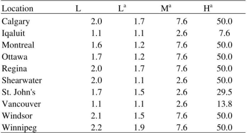
Method 2c – adjust the value of L, M, and H.Adjusting the value of the light, moderate, and heavy

amounts decreases the deviation in the difference from the annual mean when compared to the recommended values. However the method generally does not produce a significant improvement in deviation for individual months, sometimes increasing the deviation in the summer months (see Fig. 11). The results of modifying L are shown in Fig. 1 through Fig. 10. The consistent underestimation during the summer months remains. The adjusted L, M, and H values are given in Table 4. It should be noted that the effect of adjusting the M and H values did not produce the desired effect. This is due to the fact that the bulk of the observed rainfall is observed to be in the light category. Consequently most of the deviation was taken up by adjusting the L value. Adjusting the higher intensity values makes up for the left over

deviation. Since there are few occurrences of these events very large adjustments are made. The moderate category is usually pushed to the maximum limit of 7.6mm/h and the heavy category is pushed to the arbitrary limit of 50mm/h to attempt to account for any underestimate.

Method 3 – stochastic approach. In this method the values L, M, and H were assigned using a stochastic process. For each location a two-parameter Weibull distribution for rainfall intensity was determined. The results of modifying L are shown in Fig. 1 through Fig. 10. To construct a weather file each observation of rainfall in the historical data file was replaced with a random number fitting the distribution determined for each location. Two such distributions are shown in Figs. 13 and 14. The distribution parameters are given in Table 5. If the observation was ‘Light’ then a random number in the light range (1.1–2.5 mm/h) was generated. A similar procedure was used for ‘Moderate’ and ‘Heavy’ observations. This method does not significantly improve the estimate of rainfall amounts and in some cases increases the deviation in the difference from the annual mean when compared to the recommended values. For the summer months there is a slight improvement (see Fig. 11). The consistent underestimation during the summer months remains, however. The effect of adjusting the L, M and H values randomly did not produce a significant

improvement. As noted above the bulk of the observed rainfall falls in the light category. Varying the M and H values does not produce an improvement in accuracy. Assigning the light intensity randomly has the effect of smearing the error over all the months of the year and not significantly improving either the accuracy of the monthly or annual totals. The main problem of missing observations or overestimates of the intensity was not resolved. There was very little room in the range of light intensity rainfall to makeup for missing observations or an estimate bias.

FIGURE — 11. Error from long-term mean values for the month of July.

FIGURE — 12. Underestimate in measured rainfall related to mean number of thunderstorms for the 10 locations studied. The two overestimates are for Iqaluit and Vancouver the data for which is problematic.

FIGURE — 13. Weibull probability distribution of rainfall intensity for Vancouver BC.

TABLE 4 — Adjusted values of L, M, and H for the locations considered Location L La _Ma _Ha Calgary 2.0 1.7 7.6 50.0 Iqaluit 1.1 1.1 2.6 7.6 Montreal 1.6 1.2 7.6 50.0 Ottawa 1.7 1.2 7.6 50.0 Regina 2.0 1.7 7.6 50.0 Shearwater 2.0 1.1 2.6 50.0 St. John's 1.7 1.5 2.6 29.5 Vancouver 1.1 1.1 2.6 13.8 Windsor 2.1 1.5 7.6 50.0 Winnipeg 2.2 1.9 7.6 50.0

a_{Values determined by adjusting L, M, and H}

TABLE 5 — Distribution parameters shape (β) and scale (η), for the locations studied

Location β η Location β η Calgary 0.68 0.95 Shearwater 0.76 1.5 Iqaluit 0.69 0.52 St. John's 0.75 1.2 Montreal 0.61 0.91 Vancouver 0.91 1 Ottawa 0.6 0.9 Windsor 0.62 1.1 Regina 0.58 0.84 Winnipeg 0.58 0.98

Discussion

Analysis shows that there is no real substitute for measured rain data however the measurement of rainfall is a problem in itself with errors ranging up to 50%, as discussed in Section 4. In Canada many types of rain gauges have been used over the period of record covered by the archived data. Many stations used or still use a MSC Type B Standard Gauge [64], essentially a funnel and a graduated cylinder, which is read manually. This type rain gauge data is perhaps the most accurate of the generally available data, however, the data is generally reported as an accumulation of 6 h or more. Tipping bucket rain gauges (0.2 mm per tip) do provide rain intensities at hourly intervals, which is acceptable, but there are some issues with the accuracy of data especially at high rain intensities [62]. As well hourly rain intensities are sometimes adjusted to match six-hourly or daily totals from MSC Type B Standard Gauge data. The main reason this is done is to spread the systematic error related to rainfall rate across all the observations in a day [65]. Last, tipping buckets are generally shut down or fail to record accurately during cold periods, thus missing significant amounts of rain. Newer rain measuring devices, using optical occlusion or sensor plates may alleviate some of these inaccuracies.

If no intensity information and weather observation codes are available, it is possible to estimate intensity from the observations. Here however there is a possibility of discrepancies between events recorded by a rain gauge and those noted by an observer, such as the missed events discussed above. Underreporting can lead to an underestimation of rainfall in the warm months in climates where convective rainfall occurs frequently. Note the west coast of North America is an exception. Generally, there is no way to reconstruct these missing events. There is also the possibility of observer bias in overestimating the intensity of rainfall. This can lead to an overestimation throughout the year but most notably in the spring and autumn seasons. The data from Vancouver BC and Iqaluit NU seems to show this trend. Although it is possible to come close to the annual mean, such deficiencies make it difficult at best to reconstruct the monthly pattern of rainfall during the year from the observation codes. An implication for hygrothermal modeling if monthly rainfalls differ from those suggested by the observation codes is that wetting and drying spells will

Weather Observing Systems (AWOS), Automated Surface Observing Systems ASOS), and Reference Climate Stations (RCS) should remedy some of these deficiencies.

Despite the drawbacks, if only datasets with weather codes are available it is possible to estimate the rainfall intensity from the codes. The values for rainfall intensity recommended by meteorological services are acceptable in general and should be used initially [40, 65]. Given that the weather observations were originally developed for aviation purposes the fact they give a reasonable estimate is somewhat surprising. Adjusting recommended intensity values does improve the annual rainfall estimate, but not the monthly totals, which are even made worse in some instances.

Adjustments are advisable where there is evidence of bias. For example for Vancouver BC and Iqaluit NU the light intensity value, L, value should be adjusted downward. With regard to adjusting the moderate and heavy values to get close to the annual mean the moderate and heavy values should be left as

recommended. Adjustment of L is the preferred way to deal with discrepancies between yearly estimates because most events are coded as light. There is only an insignificant amount of adjustment available by changing M, or even more so, H, simply because this would affect so few events. Adjusting the M and H values to correct underestimates tends to push the values to limits of the defined ranges, producing unrealistically high values for moderate and heavy rain events.

If there is lack of guidance as to the rainfall intensity amounts then the light amount, assumed to produce the bulk of the rainfall, can be estimated from Eq. (9). This equation was developed by assuming a simple linear relation between L and ratio of long-term mean annual rainfall to the square of the long-term mean annual number of rainy days. The R2 _{for the regression is not particularly good, -0.29. Iqaluit is an outlier}

and if it is removed from the dataset the correlation improves. As noted earlier there is clearly a problem with the weather code data for Iqaluit. With Iqaluit removed the slope becomes 30.395 and the R2 _{value is}

0.77. The values for M and H can be assumed to be 5.1mm/h and 13mm/h respectively or whatever the local meteorological service recommends.

X

L

=

27

.

536

(9) 2 rainydays rain X = (10)

The stochastic model works but the results are not significantly better than adjusting the intensity values by minimizing deviation from the long-term means. Reasonable estimates for long-term rainfall and yearly totals are obtained but monthly totals are still off. The problem still remains with the stochastic method, as with the others, of dealing with missing observations and observer bias. Although meteorological service recommended values are preferable (method 2), the stochastic method can provide a data file, which gives the appearance of naturally occurring variability instead of data file where rain intensity is stepped but otherwise adds no value. It could also be used if there is no guidance for the intensity values for L, M, and H. The method is also can be used if only occurrence of rain is recorded but not the intensity. This however could introduce significant error in the rainfall amounts. The distribution parameters also need to be estimated. To estimate the rainfall intensity distribution for a given location without using tipping bucket or other short-term data, the scale parameter, η, is correlated to the ratio of mean annual rainfall to the mean annual number of rainy days. The shape parameter, β, however did not seem to correlate well with long-term rainfall parameters. A least square fit, assuming a logarithmic function, produces an equation for estimating the scale parameter, though the correlation is less than ideal (R2 _{= 0.56). If the shape is assumed}

to be constant, 0.5, for all locations, then the following simple fit, given in Eq. (11), can be used to estimate the scale parameter.

2156 . 0 ) ln( 329 . 0 + = Y η (11) rainydays rain Y = (12)

Conclusions

Rainfall intensities and wind speeds derived from 10-minute raw data have been suggested as highly desirable for hygrothermal modeling, but unless and until they are made broadly available, one must make the best possible use of what we have in Canada. The most widely available and straightforward, because accompanied by concurrent wind speed, are the qualitative rain intensities, Light, Moderate, and Heavy, with corresponding quantitative translations recommended by Environment Canada. Methods 2a, b, and c do improve agreement of individual monthly and yearly totals with long-term means determined by rain gauge measurements, but deviations remain disturbingly high in some cases.

Method 1 cannot be recommended as a stand-alone data source, but is a useful supplement to the

qualitative recommendations of Environment Canada. The main reason for this is that the rain gauges may not be co-located with the wind measurement instruments. This potentially adds to the uncertainty for hygrothermal modeling since coincident rainfall, wind speed, and wind direction are required. Where the instruments are located in proximity the records have to be synchronized as was done in this study. Even then there may be discrepancies between the records of events. Rain gauge data shortcomings are not likely to be rectified until more robust devices come into wide use as part of Automated Weather Systems. Even so, tipping bucket data helps to set up the parameters for adding random hourly components to produce a series of intensities with similar stochastic properties to actual measurements. Unfortunately, Method 3 appears to do little more than produce a plausible series of intensities to replace step changes with only three possible values.

Rainfall and wind data are the climate parameters that appear to have the greatest amount of measurement uncertainty. The uncertainty is partly due to the nature of the phenomenon and partly due to measurement difficulties. It is difficult to extrapolate how the uncertainties in rainfall data translate into uncertainties in hygrothermal simulation output. Building envelope simulations are very dependent on construction techniques as well as the interior and exterior boundary conditions. For example a wall with a drainage cavity may be relativity insensitive to rainfall whereas a wall that allows water penetration, a simulated leak, might be very sensitive variations in wind-driven rain. The findings reported here do not exhaust all avenues for making the best of available data, but the long-range plan must be to radically improve measuring equipment and data-gathering procedures. Until such a plan is realized, we conclude that Environment Canada’s recommendations (e.g. CWEEDS) for conversion of codes to intensities, adjusted to minimize differences from rain-gauge-based long-term annual means, represent the best value for effort expended.

References

[1] Karagiozis AN, Kumaran MK. Application of hygrothermal models to develop building envelope design guidelines. In: proceedings of the 4th Japan/Canada Housing R&D Workshop Sapporo, Japan: November 17, 1997, p. III-25-36.

[2] American Society of Heating Refrigeration and Air-Conditioning Engineers. ASHRAE Standard 160P Design criteria for moisture control in buildings. Public Review Draft September 2006, p. 6-7. Atlanta, GA.

[3] Kyle B, Lacasse MA, Cornick SM, Abdulghani K. A GIS-based framework for the evaluation of building façade performance and maintenance prioritization. In: proceedings of the 11th

International conference of Building Materials and Components, Istanbul Turkey May 11-14, 2008, p. 1933-1941.

[4] Lacasse MA, Kyle B, Talon A, Boissier D, Hilly T, Abdulghani K. Optimization of the building maintenance management process using a markovian model. In: proceedings of the 11th International Conference of Building Materials and Components, Istanbul Turkey: May 11-14, 2008, p. 1953-1960.

[5] Hagentoft, C-E, Adan, O, Adl-Zarrabi, B, Becker R, Brocken H, Carmeliet J, Djebbar R, Funk M, Grunewald J, Hens H, Kumaran MK, Roels S, Kalagasidis AS, Shamir D. Assessment method of numerical prediction models for combined heat, air and moisture transfer in building components:

Implementation Plan, July 22, 2003 p. 26, (Also published in Journal of Thermal Envelope and Building Science 2004; 27(4) 327-352.)

[6] Geving S, Karagiozis A, Salonvaara M. Measurements and two-dimensional computer simulations of the hygrothermal performance of a wood frame wall. Journal of Building Physics 1997; 20 301-319.

[7] Kuenzel HM, Kiessl K. Calculation of heat and moisture transfer in exposed building components. International Journal of Heat and Mass Transfer; International Journal of Heat and Mass Transfer 1997; 40(1) 159-167.

[8] Karagiozis AN. State of the art hygrothermal modeling: Building moisture analysis tutorial. Research Coordinating Committee on Moisture Building Environment and Thermal Envelope Council, September 17, 1997, p. 1-14. (NRCC-41357)

[9] Tariku F, Kumaran MK. Hygrothermal modeling of aerated concrete wall and comparison with field experiment. In: proceedings of 3rd _{International Building Physics Conference, Montreal, Canada:}

August 27, 2006, p. 321-32. (NRCC-45560) URL: http://irc.nrc-cnrc.gc.ca/pubs/fulltext/nrcc45560/

[10] CMHC. Review of hygrothermal models for building envelope retrofit analysis. Research Highlights, Technical Series 03-128, Canadian Mortgage and Housing Corporation, Ottawa Ontario.

November. 2003.

[11] Nofal M, Straver M, Kumaran MK, Comparison of four hygrothermal models in terms of long-term performance assessment of wood-frame constructions. In: proceedings of the 8th _Canadian

Conference on Building Science and Technology, Toronto Canada, February 2001. p. 118-138. [12] Djebbar R, Kumaran MK, van Reenen D, Tariku F. Use of hygrothermal numerical modeling to

identify optimal retrofit options for high-rise buildings. In: proceedings 12th _{International Heat}

Transfer Conference, Grenoble, France, August 18, 2002, p. 165-170. (NRCC-46032) URL: http://irc.nrc-cnrc.gc.ca/pubs/fulltext/nrcc46032/

[13] Finch G, Straube, J. The drying potential of wood frame rainscreen walls in Vancouver’s coastal climate. In: proceedings of the 11th _{Canadian Conference on Building Science and Technology,}

Banff Canada, March 21-23, 2007, p. 113-125

[14] Holm AH, Kuenzel HM. "Practical application of an uncertainty approach for hygrothermal building simulations-drying of an AAC flat roof." Building and Environment 2002; 37(8) 883-889. [15] Samuelson I. Hygrothermal performance of attics. Journal of Building Physics1998; 22 132-146. [16] Bomberg M, Kumaran MK, Day K. Moisture management of EIFS walls-- Part 1: The basis for

evaluation. Journal of Building Physics 1999; 23. 78-94.

[17] Salonvaara M, Nieminen J. Hygrothermal performance of a new light gauge steel-framed envelope system. Journal of Building Physics 1998; 22 169-182.

[18] Kalamees T, Vinha J. Hygrothermal calculations and laboratory tests on timber-framed wall structures. Building and Environment 2006; 38(5) 689-697.

[19] Teasdale St Hilaire A, Derome D. Comparison of experimental and numerical results of wood-frame wall assemblies wetted by simulated wind-driven rain infiltration. Energy and Buildings 2007; 39(11) 1131-1139.

[20] Nofal M, Morris PI. Criteria for unacceptable damage on wood systems. In: proceedings Japan-Canada Conference on Building Envelope, Vancouver Canada, June 04, 2003, p. 1-14. (NRCC-45140) URL: http://irc.nrc-cnrc.gc.ca/pubs/fulltext/nrcc45140/

[21] Sedlbauer K. Prediction of mould growth by hygrothermal calculation. Journal of Thermal Envelope and Building Science 2002; 25 321-336.

[22] Karagiozis A, Salonvaara M. Hygrothermal system-performance of a whole building. Building and Environment 2001; 36(6) 779-787

[23] Pavlik Z, Pavlik J, Jirickova M, Cerny R

.

System for testing the hygrothermal performance of multi-layered building envelopes. Journal of Thermal Envelope and Building Science 2002; 25 239-249. [24] Barbosa RM, Mendes N. Combined simulation of central HVAC systems with a whole-building

hygrothermal model. Energy and Buildings 2008; 40(3) 276-288.

[25] Rode C, Grau K. Moisture buffering and its consequence in whole building hygrothermal modeling. Journal of Building Physics: 2008; 31 333-360.

[26] Abadie MO, Mendonc-a KC. Moisture performance of building materials: From material

characterization to building simulation using the Moisture Buffer Value concept. Building and Environment (2008), doi:10.1016/j.buildenv.2008.03.015

[27] Blocken B, Roels S, Carmeliet J. A combined CFD–HAM approach for wind-driven rain on building facades, Journal of Wind Engineering and Industrial Aerodynamics 2007; 95 585–607

[28] Cornick SM, Djebbar R, Dalgliesh WA. Selecting moisture reference years using a moisture index approach. Building and Environment 2003; 38:(12) 1367-1379.

[29] Sanders C. Environmental Conditions, Final Report: Task 2. International Energy Agency. Energy Conservation in Buildings and Community Systems, Annex 24 Heat-Air and Moisture Transfer in Insulated Envelope Parts (HAMTIE). Laboratorium Bouwfysica, K.U.-Leuven, Belgium, 1996. [30] Salonvaara M, Pezoulas L, Zhang J,. Oazera M. 1325-RP Environmental Weather Loads for

Hygrothermal Analysis and Design of Buildings. Final Report. American Society of Heating Refrigeration and Air-Conditioning Engineers, Atlanta, GA. 2009.

[31] Kumaran MK, Mukhopadhyaya P, Cornick SM, Lacasse MA, Rousseau MZ, Maref W, Nofal M, Quirt JD. Dalgliesh WA. An Integrated methodology to develop moisture management strategies for exterior wall systems. In: proceedings of the 9th _{Canadian Conference on Building Science and}

Technology, Vancouver Canada, February 27, 2003. p. 45-62. (NRCC-45987) URL: http://irc.nrc-cnrc.gc.ca/pubs/fulltext/nrcc45987/

[32] Lacy RE. Driving-rain maps and the onslaught of rain on buildings. In: proceedings of the RILEM/CIB Symposium on Moisture Problems in Buildings, Helsinki Finland, 1965. [33] Choi ECC. Determination of wind-driven rain intensity on building faces. Journal of Wind

Engineering and Industrial Aerodynamics 1994; 51 55-69.

[34] Straube JF, Burnett EFP. Simplified prediction of driving rain deposition. Proceedings of International Building Physics Conference, Eindhoven, the Netherlands, September 18-21, 2000, pp. 375-382. [35] National Oceanic and Atmospheric Administration. Solar and Meteorological Surface Observational

Network 1961-1990 Version 1.0, September 1993. National Climatic Data Center Federal Building 151 Patton Avenue, Asheville NC, USA, 28801-5001.

[36] National Oceanic and Atmospheric Administration. Hourly United States Weather Observations, 1990-1995, October 1997. National Climatic Data Center Federal Building 151 Patton Avenue Asheville NC USA, 28801-5001.

[37] Environment Canada. Canadian Weather Energy and Engineering Data Sets Revise on April 30,2003. Atmospheric Environment Service, Environment Canada 4905 Dufferin Street, Toronto, Canada M3H 5T4

[38] Stoffel TL, Rymes MD. Production of the Weather Year for Energy Calculations Version 2 (WYEC2)

Data Sets. ASHRAE Transactions 1998;104(2):487-497.

[39] Atmospheric Environment Services. Software Implementation for Climatological Ice Accretion Modelling Project. Internal Report to Energy and Industrial Applications Section. Canadian Climate Center. Toronto Canada, 1984, p. 157.

[40] Environment Canada. Manual of Service Weather Observations (MANOBS). Atmospheric Environment Service. Central Service Directorate. Toronto. Ontario. 1987.

[41] Cornick SM, Maref W, Abdulghani K, van Reenen D. 1-D hygIRC: a simulation tool for modeling heat, air and moisture movement in exterior walls. Building Science Insight 2003 Seminar Series October 01, 2003, p. 1-10. URL: http://irc.nrc-cnrc.gc.ca/pubs/fulltext/nrcc46896/: for 1-D hygIRC see http://irc.nrc-cnrc.gc.ca/bes/software/hygIRC/index_e.html

[42] Cornick SM, Lacasse MA. A review of climate loads relevant to assessing the water tightness performance of walls, windows and wall-window interfaces. Journal of ASTM International, 2:(10) 2005. p. 1-16. URL: http://irc.nrc-cnrc.gc.ca/pubs/fulltext/nrcc47645/

[43] Blocken B, Carmeliet J. Driving Rain on Building Envelopes- I. Numerical Estimation and Full-Scale Experimental Verification. Journal of Building Physics 2000; 24 61-85.

[44] Blocken B, Carmeliet J.. Driving rain on building envelopes – II. Representative experimental data for driving-rain estimation. Journal of Thermal Envelope and Building Science 2000; 24:(2) 89-110, [45] Sumner G. Precipitation process and analysis. John Wiley and Sons Chichester UK 1988.

[46] Makhuvha T, Pegram G, Sparks R, Zucchini W. Patching rainfall data using regression models: Part 2, Comparison of accuracy, bias and efficiency. Journal of Hydrology 1997; 198 308-318.

[47] Acock M, Pachepsky Y. Estimating missing weather data for agricultural simulations using group method of data handling. Journal of Applied Meteorology 1999; 39(7) 1176-1184.

[48] Baltazar J, Claridge D. Restoration of short periods of missing energy use and weather data using cubic spline and fourier series approaches: Qualitative analysis. In: proceedings of the 13th Symposium on Improving Building Systems in Hot and Humid Climates, May 20-23, 2002, Houston, TX, p. 213-218.

[49] Koronthályová OG, Matiašovský P. Driving rain course simulation based on daily data. Journal of Thermal Envelope and Building Science2001; 25 51-66.

[50] Matiašovský P. Koronthályová OG. Sensitivity analysis of hygrothermal performance of an external wall to uncertainty of driving rain data. In: proceedings of the International Building Physics Conference. Technische Universiteit Eindhoven. 18-21 September, 2000, pp. 589–595. [51] Blocken B, Carmeliet J. On the errors associated with the use of hourly data in wind-driven rain

calculations on building facades, Atmospheric Environment 41 2007; 2335–2343.

[52] Blocken, B, Carmeliet J. A review of wind-driven rain research in building science. Journal of Wind Engineering and Industrial Aerodynamics 2004; 92(13) 1079-1130.

[53] Welsh LE, Skinner WR, Morris RJ. A climatology of driving rain wind pressure for Canada. Environment Canada, Atmospheric Environment Service, Climate and Atmospheric Research Directorate Draft Report, 1989.

[54] Skerlj P. A critical assessment of the driving-rain wind pressures used in CSA Standard A440. Master’s Thesis, Boundary Layer Wind Tunnel University of Western Ontario, Canada. [55] Beaulieu P, Bomberg MT, Cornick SM, Dalgliesh WA, Desmarais G, Djebbar R, Kumaran MK,

Lacasse MA, Lackey JC, Maref W, Mukhopadhyaya P, Nofal M, Normandin N, Nicholls M, O'Connor T, Quirt JD, Rousseau MZ, Said MN, Swinton MC, Tariku F, van Reenen D. Final Report from Task 8 of MEWS Project (T8-03) – Hygrothermal response of exterior wall systems to climate loading: Methodology and interpretation of results for stucco, EIFS, masonry and siding-clad wood-frame walls. Research Report RR-118, Institute for Research in Construction, National Research Council Canada, November 01, 2002 (RR-118). URL:

http://irc.nrc-cnrc.gc.ca/pubs/rr/rr118/

[56] Dalgliesh WA, Ranking of climate severity in Canada for rain penetration control – Report # 2, T.G. 4, Mews Memorandum #3. personal communication, June 28, 1989.

[57] Canadian Commission on Building and Fire Codes, National Research Council of Canada. National Building Code of Canada 2005. Ottawa, Volume 1: Division B, Appendix C, Table 9.25.1.2, p. 9-141.

[58] Hubbard KG, Kunkel KE, DeGaetano AT, Redmond KT. Sources of uncertainty in the calculation of design weather conditions. ASHRAE Transactions 2005; 111 (2) 317-326.

[59] Henderson-Sellers A, Robinson PJ, Contemporary climatology 2nd _{Edition, Longman, Harlow, Essex,}

England 1999. Ch. 5.

[60] Habib E, Krajewski WF, Kruger A. Sampling errors of tipping-bucket rain gauge measurements. Journal of Hydrologic Engineering, March/April 2001, p. 159-166.

[61] Curtis D, Burnash RJC. Inadvertent rain gauge inconsistencies and their effect on hydrologic analysis David C. Curtis DC Consulting 9477 Greenback Lane, Suite 523A Folsom, CA 95630 Tel: 916-988-2771, E-mail dccurtis@pacbell.net, Robert J. C. Burnash NWS (retired).

http://www.onerain.com/includes/pdf/whitepaper/InconsistentRainGageRecords.pdf [62] Sevruk B. Methods of correction for systematic error in point precipitation measurement for

operational use. Operational Hydrology Report 21. World Meteorological Organization. Geneva, Switzerland. 1982.

[63] Devine KA, Mekis É. Field accuracy of Canadian rain measurements. Atmosphere-Ocean 2008; 46(2) 213–227.

[64] Morris RJ. Personal communication. Environment Canada 4905 Dufferin Street, Toronto, Ontario M3H 5T4. October 24, 2007.