HAL Id: inria-00321503
https://hal.inria.fr/inria-00321503
Submitted on 16 Feb 2011HAL is a multi-disciplinary open access
archive for the deposit and dissemination of sci-entific research documents, whether they are pub-lished or not. The documents may come from teaching and research institutions in France or abroad, or from public or private research centers.
L’archive ouverte pluridisciplinaire HAL, est destinée au dépôt et à la diffusion de documents scientifiques de niveau recherche, publiés ou non, émanant des établissements d’enseignement et de recherche français ou étrangers, des laboratoires publics ou privés.
Jakob Verbeek, Nikos Vlassis, Ben Krose
To cite this version:
Jakob Verbeek, Nikos Vlassis, Ben Krose. Procrustes analysis to coordinate mixtures of probabilistic principal component analyzers. [Technical Report] IAS-UVA-02, 2002, pp.18. �inria-00321503�
Intelligent
Autonomous
Systems
IAS technical report series, nr. IAS-UVA-02-01
Procrustes Analysis to Coordinate Mixtures of
Probabilistic Principal Component Analyzers
J.J. Verbeek, N. Vlassis and B. Kr¨ose
Computer Science Institute Faculty of Science
University of Amsterdam The Netherlands
Mixtures of Probabilistic Principal Component Analyzers can be used to model data that lies on or near a low dimensional manifold in a high dimensional obser-vation space, in effect tiling the manifold with local linear (Gaussian) patches. In order to exploit the low dimensional structure of the data manifold, the patches need to be localized and oriented in a low dimensional space, so that ‘local’ co-ordinates on the patches can be mapped to ‘global’ low dimensional coco-ordinates. As shown by [Roweis et al., 2002], this problem can be expressed as a penalized likelihood optimization problem. We show that a restricted form of the Mix-tures of Probabilistic Principal Component Analyzers model allows for an efficient EM-style algorithm. The Procrustes Rotation, a technique to match point con-figurations, turns out to give the optimal orientation of the patches in the global space. We also show how we can initialize the mappings from the patches to the global coordinates by learning a non-penalized density model first. Some experi-mental results are provided to illustrate the method.
Keywords: dimension reduction, feature extraction, principal manifold, selforga-nization
Contents
1 Introduction 1
2 The density model 1
3 A simplified algorithm due to simplified density model 2 3.1 Objective Function . . . 2 3.2 Optimization . . . 4
4 Initialization from a data-space mixture 5
4.1 Fixing the data-space mixture . . . 5 4.2 Optimization and Initialization . . . 6
5 Experimental results 6
5.1 Artificial data-set . . . 6 5.2 Images of faces . . . 6 5.3 Robot navigation . . . 9
6 Discussion and conclusions 9
A GEM for constrained MPPCA 11
A.1 Updating the loading matrices . . . 12 A.2 Variance inside and outside the subspace . . . 12
B A variation on weighted Procrustes analysis 13
Intelligent Autonomous Systems Computer Science Institute
Faculty of Science University of Amsterdam Kruislaan 403, 1098 SJ Amsterdam The Netherlands tel: +31 20 525 7461 fax: +31 20 525 7490 http://www.science.uva.nl/research/ias/ Corresponding author: J.J. Verbeek tel: +31 (20) 525 7515 [email protected] http://carol.science.uva.nl/~jverbeek/
Section 1 Introduction 1
1
Introduction
With increasing sensor capabilities, powerful feature extraction methods are becoming increas-ingly important. Consider a robot sensing its environment with a camera yielding a stream of 100× 100 pixel images, i.e. a stream of 10.000 dimensional vectors if we regard the image as a pixel intensity vector. The observations made by the robot often have a much lower intrinsic dimensionality. If we assume a fixed environment, and a robot that can rotate around its axis and drive through a room, the intrinsic dimensionality is only three. Linear feature extraction techniques are able to do a fair compression of the signal by mapping it to a much lower di-mensional space. However, only in very few special cases the manifold on which the signal is generated is a linear subspace of the sensor space. This clearly limits the use of linear techniques and suggests to use non-linear feature extraction techniques.
Mixtures of Factor Analyzers (MFA) [Ghahramani and Hinton, 1996] and Mixtures of Prob-abilistic Principal Component Analyzers (MPPCA) [Tipping and Bishop, 1999] can be used to model such non-linear data manifolds. These methods (in fact MPPCA is a special case of MFA) provide a mapping back and forth between latent and data-space. However, these mappings only have a local applicability and are not related, i.e the coordinate systems of neighboring facor analyzers might be completely differently oriented. We cannot combine the different latent spaces, the coordinates of a point in one subspace give no infotmation on the coordinates in a neighboring subspace.
Recently, a model was proposed that integrates the local linear models into a global latent space, allowing for mapping back and forth between the latent and the data-space. The idea is that there is a linear map for each factor analyzer between the the data-space and the global latent space. This penalized log-likelihood model proposed in [Roweis et al., 2002], solved by an EM-like procedure, is discussed in the next section.
Here, we show how we can remove the iterative procedure from the M-step by simplifying the density model. Furthermore, we show how we can use an ‘uncoordinated’ mixture model to initialize the mappings from data to latent space, providing an alternative to using an external (unsupervised) method to initialize the latent coordinates for all the data points.
In the next section, we describe the density model that is used. Then, in Section 3 we show how this density model removes one of the iterative procedures in the algorithm given in [Roweis et al., 2002]. Section 4 discusses how an ‘uncoordinated’ mixture model can be used to initialize the mappings between latent and data-space. Some experimental results are given in 5. We end with a discussion and some conclusions in 6.
2
The density model
To model the data density in the high dimensional space we use mixtures of a restricted type of Gaussian densities. The mixture is formed as a weighted sum of its component densities, the weight of each component is called its ‘mixing weight’ or ‘prior’. The covariance matrices of the Gaussians are constrained to be of the form:
C= σ2(ID + ρΛΛ>), Λ>Λ= Id, ρ > 0 (1)
where D and d are respectively the dimension of the high-dimensional/data-space and the low-dimensional/latent space. We use Id to denote the d-dimensional identity matrix. The columns
of Λ, in factor analysis known as the loading matrix, are D-dimensional vectors spanning the subspace. Directions within the subspace have variance σ2(1 + ρ), other directions have σ2
variance. This is as the Mixture of Probabilistic Principal Component Analyzers (MPPCA) model, with the difference that here we do not only have isotropic noise outside the subspaces
but also also isotropic variance inside the subspaces. We use this density model to allow for con-venient solutions later. In Appendix A we derive a Generalized EM algorithm to find maximum likelihood solutions for this model.
The same model can be rephrased using hidden variables z, which we use to denote ‘internal’ coordinates of the subspaces. We scale the coordinates z such that:
p(z| s) = N (0, Id), (2)
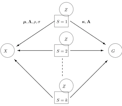
whereN (µ, Σ) denotes the Gaussian density, centered at µ and with covariance matrix Σ. The internal coordinates allow us to clearly express the link to the global latent space, for which we denote coordinates with g. All mixture components/subspaces have their own orthogonal mapping to the global space, parameterized by a translation κ and a matrix A, i.e. p(g| z, s) = δ(κs + Asz), where δ(·) denotes the distribution with mass 1 at the argument. We use ps
to denote the mixing weight of mixture component/subspace s and µs to denote its mean or location. The generative model then looks like:
p(x) =X s psN (µs, σs2(ID + ρsΛsΛ>s)) = X s ps Z zdz p(x| z, s)p(z | s) (3) p(x| z, s) = N (µs+√ρsσsΛsz, σs2ID) (4) p(g) = X s psN (κs, AsA>s) = X s psN (κs, α2sσs2ρsId). (5)
We put an extra constraint on the projection matrices:
As = αsσs√ρsRs, R>sRs= Id, αs> 0. (6)
The matrix Rs implements only rotations plus reflections due to the orthonormality constraint.
The generative model reads: first ‘nature’ picks a subspace according to the prior distribution {ps}. A subspace generates internal coordinates z , which on the one hand give rise to hidden
global coordinates g (via the translation κs and the rotation plus scaling As) and on the other
hand to observable data x (via the translation µs and the orthogonal mapping √ρsσsΛs) plus
some noise with covariance σ2ID. Figure 1 illustrates the model. Note that the model assumes that locally there is a linear correspondence between the data space and the latent space. Fur-thermore, note that the densities p(g | x, s) and p(x | g, s) are Gaussian densities and hence that p(g | x) and p(x | g) are mixtures of Gaussians. In the next section we discuss how this density model differs from [Roweis et al., 2002].
3
A simplified algorithm due to simplified density model
The goal is, given observable data {xn}, to find a good density model in the data-space and
mappings{As, κs} that give rise to ‘consistent’ estimates for the hidden {gn}. With consistent
we mean that if a point x in the data-space is well modeled by two subspaces, then the corre-sponding estimates for its latent coordinate g should be close to each other, i.e. the subspaces should ‘agree’ on the corresponding g.
3.1 Objective Function
To measure the level of agreement, one can consider for all data points how uni-modal the distribution p(g| x) is. This idea was also used in [Vlassis et al., 2002], there the goal was to find orhtogonal projections for supervised data, such that the projections from high to low dimension preserve the manifold structure. In [Roweis et al., 2002] it is shown how the double objective
Section 3 A simplified algorithm due to simplified density model 3 ÁÀ ¿ ÁÀ ¿ ÁÀ ¿ ÁÀ ¿ ÁÀ ¿ ¾ @ @ @ @ @ @ @ @ @ I QQ QQ QQ QQ Q s -¡¡ ¡¡ ¡¡ ¡¡¡ µ ´ ´ ´ ´ ´ ´ ´ ´ ´ + S = k G S = 2 Z Z X µ, Λ, ρ, σ κ, A Z S = 1
Figure 1: The generative model: x and g are independent given s, z.
of likelihood and uni-modality can be implemented as a penalized log-likelihood optimization problem.
Let Q(g | xn) denote a Gaussian approximation of p(g | xn) = Psp(g | xn, s)pns = P
sp(g, s| xn), with pns= p(s| xn). We define:
Q(g, s| xn) = Q(s| xn)Q(g| xn), (7)
where Q(g| xn) =N (gn, Σn) and Q(s| xn) = qns. As a measure of uni-modality we can use a
sum of Kullback-Leibler divergences:
X ns Z g Q(g, s| xn) log " Q(g, s| xn) p(g, s| xn) # dg= (8) X n DKL({qns} k {pns}) + X s qnsDns, (9)
where Dns = DKL(Q(g | xn) k p(g | xn, s)). The total objective function, combining
log-likelihood and the penalty term, then becomes:
Φ= X n log p(xn)− DKL({qns} k {pns}) − X s qnsDns (10) = X ns Z g dg Q(g, s| xn)[− log Q(g, s | xn) + log p(xn, g, s)] (11)
The form of (11) shows that we can view this as a variational approach to fit the mixture model where we consider both s and g as hidden variables. We approximate the true p(g, s| x) with the ‘simple’ Q(g, s| x). The terms involving the mixture model p, represent the expected likelihood. The penalty term makes the distributions Q(g, s| xn) mimmic the distributions p(g, s| xn).
Our density model differs with that of [Roweis et al., 2002] in two aspects:
1. isotropic noise model outside the subspaces (as opposed to diagonal covariance matrix)
As a result, orthogonal mappings from the subspaces to the latent space can be absorbed in the matrices Λ, since for orthogonal matrices R we have ΛR>(ΛR>)>= ΛΛ>, i.e. the density
model does not change if we replace Λ with ΛR>. Also, using our density model it turns out that to optimize Φ with respect to Σn, it should be of the form1 Σn = βn−1Id. Therefore we
work with βn from now on.
Using our density model we can rewrite the objective function (up to some constants) as:
Φ= X ns qns " − d2log βn− log qns− ens 2σ2 s − vs 2 h dβ−1n +g > nsgns ρs+ 1 i (12) −D log σs+ d 2log vs ρs+ 1 + log ps # , (13)
where we used the following abbreviations:
gns= gn− κs, xns= xn− µs, ens=k xns− α−1s ΛsRs>gnsk2, vs= ρs+ 1 σ2 sρsαs2 . (14) 3.2 Optimization
Next, we give an EM-style algorithm to optimize Φ, it is a simplified version of the algorithm provided in [Roweis et al., 2002]. The simplifications are: (i) the iterative process to solve for the Λs, Asis no longer needed; an exact update is possible and (ii) the E-step no longer involves
matrix inversions.
The same manner of computation is used: in the E-step, we compute the uni-modal dis-tributions Q(s, g | xn), parameterized by βn, gn and qns. Let hgnis = Ep(g|xn,s)[g] denote the expected value of g given xn and s. We used the following identities in the E-step update
equations: hgnis= κs+ RsΛs>xnsαsρs/(ρs+ 1), (15) Dns= vs 2[dβ −1 n +k gn− hgnis k2] + d 2[log βn− log vs]. (16) The approximating distributions Q can be found by iterating the fixed-point equations given below. Due to the form of the update for qns it seems to make sense to initialize the qnsat pns.
βn= X s qnsvs, gn= βn−1 X s qnsvshgnis, qns= pnsexp−Dns P s0pns0exp−Dns0 . (17)
In the M-step, we update the parameters of the mixture model: ps, µs, κs, ΛsRs, σs, ρs. Again
we use some compacting notation:
Cs= X n qnsk gnsk2, Es= X n qnsens, Gs= d X n qnsβ−1n (18)
Then, the update equations are:
ps= P nqns P ns0qns0 , κs= P nqnsgn P nqns , µs= P nqnsxn P nqns , (19) αs= Cs+ Gs P nqns(gns>RsΛ>sxns) , ρs= D(Cs+ Gs) d(α2 sEs+ Gs) , σ2s = Es+ ρ −1 s α−2s [Cs+ (ρs+ 1)Gs] (D + d)Pnqns (20) 1
Once we realize that the matrices Vs in [Roweis et al., 2002] are of the form cId with our density model, it
Section 4 Initialization from a data-space mixture 5
Note that the above equations require Es which in turn requires the ΛsRs via equation (14).
To find RsΛ>s we have to minimize: X n qnsens= X n qnsk xns− α−1s ΛR>gnsk2 or equivalently: − X n qnsg>ns(RsΛ>s)xns. (21)
This problem is known as the ‘weighted Procrustes rotation’ [Cox and Cox, 1994]. Let
C= [√q1sx1s· · ·√qnsxns][√q1sg1s· · ·√qnsgns]>, with SVD: C = ULΓ>, (22)
where the gns have been padded with zeros to form D-dimensional vectors, then the optimal
ΛsR>s is given by the first d columns of U Γ>.
4
Initialization from a data-space mixture
To initialize the optimization procedure described in the previous section, we can go two ways. The two ways correspond to starting with an E-step or with an M-step. In [Roweis et al., 2002] it is proposed to start with an M-step, requiring initial estimates for the global coordinates gn. The initial global coordinates are typically provided by an ‘external’ unsupervised pro-cedures, examples are LLE and Isomap. However, such methods might suffer from bad time complexity scaling with increasing sample-size2. In this section we introduce an alternative ini-tialization, that starts the update procedure with an E-step. This requires we find a data-space mixture model first, we can use the GEM algorithm described in Appendix A. Note that the greedy initialization method described in [Verbeek et al., 2001a], that builds the mixture model component-wise in order to avoid problems due to ‘unlucky’ random initialization of the mixture, can be directly used for the mixtue model described here.
4.1 Fixing the data-space mixture
Next, we consider how we can simplify the objective (13), if we fix the data-space mixture model. In this case the problem reduces to find appropriate mappings{κs, As}. Since the data-space
mixture is fixed the log-likelihood term is constant and the objective reduces to the penalty term (9). If the density model is fixed, we can reduce the number of free parameters in (9) by setting qns= pns. This simplifies (9) to:
X ns
pnsDns. (23)
Furthermore, we replace the Gaussian Q(g| xn) with a delta-peak distribution on its center gn,
this removes the free parameters Σn. This amounts to simplifying (23) further to a weighted
sum of log-likelihoods:
X n,s
pnslog p(gn| xn, s) (24)
The posterior distribution p(z| x, s) on internal coordinates z given a data point x is a Gaussian and hence also the posterior p(g| x, s) is a Gaussian. The covariance of the posterior p(z | x, s) is Id/(ρs+ 1) and to get the covariance for g we only have to multiply this with the square of
the scaling factor of As which yields: Idα2sσs2ρs/(ρs+ 1) = Idvs−1
2
4.2 Optimization and Initialization
Global maximization of (24) over all parameters is hard. Therefore, we maximize by alternating maximization over the global coordinate point estimates {gn}, and then over the patch
loca-tions and rotaloca-tions {κs, Rs}. This leads to a local maximum of the objective. Skipping some
constants, we rewrite (24) as:
−12X
n,s
pns[2d log α + vsk hgnis− gnk2 ]. (25)
In Appendix B we show how to find locally optimal parameters. Note that if the mixture in the data-space is kept fixed, then all computations involve d dimensional vectors and matrices, as expected.
Finally, to initialize the mappings we take component-wise approach, using the already initialized components to initialize the next. Note that due to the invariance w.r.t. global translations and rotations of the objective (24), we can simply initialize the first component with R = Id, α = 1, κ = 0. To initialize a new component s, we compute Rs, αs, κs which
maximize: X n h X i∈F pni i pnslog p(gn| xn, s), (26)
where F is the set of components for which we already fixed the mapping, i.e. the weights pns
are rescaled according to the already initialized components. Again, the solution is found in Appendix B. Note that these weights emphasize the data ‘on the border’ between the subspace s and the already initialized subspaces. In order to select the next subspace to initialize, we could for example pick
s = arg max s X n pns X i∈F pni/ps. (27)
This method somewhat resembles the method described in [Verbeek et al., 2001b]. There, also a similar density model is learned and then fixed to compute how the different local models can be combined into a global structure. The method presented here is more robust and applicable to any latent dimensionality.
5
Experimental results
In this section we discuss three experiments to illustrate the method. The first concerns arti-ficially generated data. The other two experiments deal with mapping sets of images to low dimensional coordinates.
5.1 Artificial data-set
As a first experiment we used an artificially generated data-set, depicted in Figure 2. We learned a mixture model with 20 components and initialized the mappings to the latent space from the data-space mixture. For all data points we also have the coordinates on the surface, so we can inspect correlation coefficients with the discovered latent coordinates. The correlation coefficient between the first latent dimension and the surface coordinates are: 0.0494 and 0.9997. For the second latent dimension these are: 0.9961 and -0.0030.
5.2 Images of faces
For this experiment we captured gray valued images of a face with a webcam. Each image of 40× 40 pixels is treated as a 1600-dimensional vector, with each coordinate describing the gray value of a specific pixel.
Section 5 Experimental results 7
Figure 2: An artificially generated data set, 1000 points in 3d on a 2d surface.
Figure 3: Images selected at equally space intervals in the discovered latent space.
Looking from left to rigth In the first experiment we used a set of 100 images of a face where there was only one degree of freedom in the data: the face was rotated from left to right when capturing the images. First we mapped the data to a 5 dimensional sub-space with PCA, capturing over 68% of the total variance in the data. Then we learned a coordinated mixture of principal component analyzers, the latent dimensionality was set to one and we used eight mixture components. To initialize, we used the method described in Section 4. The data-space mixture was learned with the greedy method of [Verbeek et al., 2001a], this method builds the mixture component per component to avoid bad initialization of the parameters. In figure 3 we show some of the used images, they are ordered according to the 1-d latent representation found by our method.
Two degrees of freedom Next, we consider a data set similar to the previous, except that the face now has a second degree of freedom, namely looking up and down. First we learned a coordinated mixture model with 1000 randomly selected images from a set of 2000 images of 40× 40 pixels each. Again, we used a PCA projection, in this case to 22 dimensions, preserving over 70% of the variance in the data set. We used a latent dimensionality of two and 20 mixture components.
Here we initialized the coordinated mixture model by clamping the latent coordinates gnat
coordinates found by Isomap and clamping the βn at small values for 50 iterations. The qns
were initialized at random values, and updated from the start. After the first 50 iterations, we also updated the βn and gn. The obtained coordinated mixture model was used to map the
remaining 1000 images, the ‘test-set’ into the latent space. For each image xn we can compute
p(g| xn), as described in Section 3 this distribution can be approximated with a single Gaussian
Qn= arg minQDKL(Qk p(g | xn)) with a certain mean and variance. We used the mean of Qn
as the latent coordinate for an image.
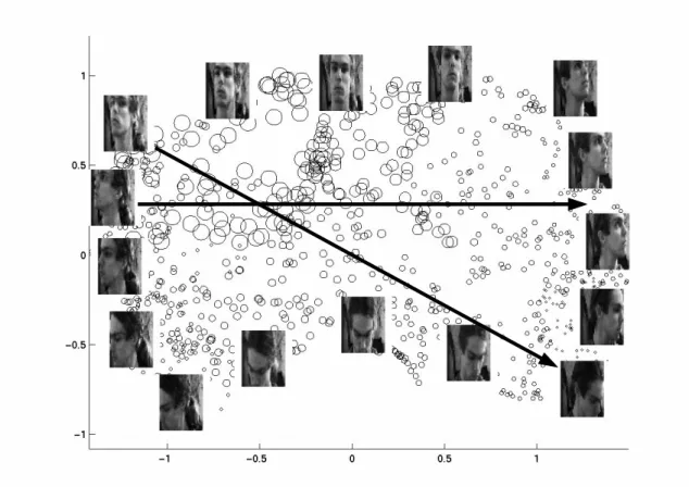
In Figure 4 we show the latent coordinates for the test-set. We observe that a sensible 2-dimensional parametrization is found in the training data set, that generalizes to the test set. To illustrate the discovered parametrization further, two examples of linear traversal of the latent space are given in Figure 5.
Figure 4: The latent coordinates for the test set. Each circle represents a latent coordinate (its center) and the uncertainty β on it (the radius of the circle is β−1/2). For some coordinates we
displayed the corresponding image at the coordinate.
Figure 5: Examples of linear traversal of the latent space. The followed trajectories correspond to the arrows in Figure 4.
Section 6 Discussion and conclusions 9
Figure 6: An example of a panoramic image as used by the robot.
5.3 Robot navigation
Here we consider images obtained from a omni-directional camera3 mounted on a mobile robot. These images are warped to gray-scale panoramic images of 256× 64 pixels, an example of such an image is given in Figure 6. The robot was placed at many locations in an office, while the orientation of the robot was kept fixed. At each location the position of the robot was recorded together with an image taken at that position.
First we consider data obtained from a rectangular area of an office, approximately 8× 112
meters wide. The robot recorded images on a 10×10 centimeter grid, in the corridor we obtained 970 images. A uniformly random selected subset of 500 of those images were used to train the coordinated mixture model, with latent dimension two and 20 mixture components. Since we have ’supervised’ data here, we can set and keep fixed the gn here at the recorded positions of
the robot. In case of significant errors in the recorded positions we might only use them for initialization. Prior to training the model, we projected the images to a 15 dimensional space capturing over 70% of the variance in the total 16.384 dimensions.
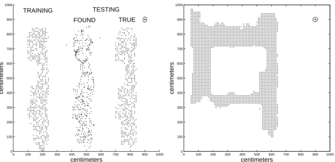
We mapped the test set to the latent space as described in the previous section. The covariance of the error between the true location and the found latent coordinates is almost diagonal with standard deviations of 13 and 17 centimeters in respectively the horizontal and vertical direction. The ellipse in Figure 7 illustrates the covariance structure, the axes of the ellipse are parallel to the eigenvectors of the covariance matrix, and their lengths equal to square root of the corresponding eigenvalues.
The same experiment was repeated with a data from a larger region, see the right pannel in Figure 7. Here the images were projected on a 50-dimensional space and 50 mixture components were used. From the total 2435 images 1700 were used for training and 735 for testing. In this experiment, the standard deviation of the error along the eigenvectors of the covariance matrix was 15 and 17 centimeters.
Although these results are good, considering that only linear models are used, we found it very hard to get good environment representation when not using the supervised position information.
6
Discussion and conclusions
Discussion In the previous section we showed examples of application of the model to visual data. Both supervised and unsupervised data sets were used. The mains reason for applying this model to supervised data instead of other regression methods are the compact decription of the mapping between the high and low dimensional space, the probabilistic framework in which it is stated and the simplicity in terms of computational effort of the mapping.
One might consider applying this method to partially supervised data sets (only a limited number of measurements is provided together with a ‘supervised’ latent coordinate). This possibility forms a line of further research.
Another future line of research is the use of the decribed density model to get an idea of the 3
0 100 200 300 400 500 600 700 800 900 1000 0 100 200 300 400 500 600 700 800 900 1000 centimeters centimeters TRAINING TESTING FOUND TRUE 0 100 200 300 400 500 600 700 800 900 1000 0 100 200 300 400 500 600 700 800 900 1000 centimeters centimeters
Figure 7: Positions in the robot navigation task. The training locations are shown left, the found locations for the test set are shown in the middle with the original locations right. The ellipse (top right) shows the covariance structure in the error. The right pannel shows the locations and error covariance for the second experiment.
(local) latent dimensionality. If we treat the latent dimensionality a unknown, we could try to estimate it by checking at the M step in an EM procedure for every component which latent dimensionality maximizes log-likelihood. As opposed to th MPPCA anf MFA density models, with our density model the covariance matrices do not form a nested family. With MPPCA and MFA the covariance matricesCd for latent dimensionality d are included in the covariance
matrices for latent dimensionality d0 > d: Cd⊂ Cd0. Hence with MPPCA and MFA, increasing the latent dimensionality can only increase the likelihood.
An important issue, not addressed here, is that is many cases where we collect data from a systems with only few degrees of freedom we actually collect one or more sequences of data. If we assume that the system can vary its state only in continuous manner, these sequences should correspond to paths on the manifold of observable data. This fact might be exploited to find low dimensional embeddings of the manifold.
Conclusions We showed how a special case of the density model used in [Roweis et al., 2002] leads to a more efficient algorithm to coordinate probabilistic local linear descriptions of a data manifold. The M-step can be computed at once, the iterative procedure to find solutions for a Riccati equation is no longer needed. Furthermore, the update equations do not involve matrix inversions anymore. However, still d singular values of a D× D matrix have to be found.
We prosposed an alternative initialization scheme for the mapping from high to low dimen-sion, that exploits the structure of a mixture model in the data space. We showed experimental results of this method discovering succesfully the structure in a data set of images of a face that rotates over its length axis. We showed how we can use the coordinated mixture model to map supervised data (robot navigation) and data for which we have uncertain latent coordinates (the 2 degrees of freedom facial images).
REFERENCES 11
References
[Cox and Cox, 1994] T.F. Cox and M.A.A. Cox. Multidimensional Scaling. Number 59 in Monographs on statistics and applied probability. Chapman & Hall, 1994.
[Ghahramani and Hinton, 1996] Z. Ghahramani and G.E. Hinton. The EM Algorithm for Mix-tures of Factor Analyzers. Technical Report CRG-TR-96-1, University of Toronto, 1996.
[Roweis et al., 2002] S. Roweis, L. Saul, and G.E. Hinton. Global coordination of local linear models. In T.G. Dietterich, S. Becker, and Z. Ghahramani, editors, Advances in Neural Information Processing Systems, volume 14, pages x–y. MIT Press, 2002.
[Tipping and Bishop, 1999] M.E. Tipping and C.M. Bishop. Mixtures of probabilistic principal component analysers. Neural Computation, 11(2):443–482, 1999.
[Verbeek et al., 2001a] J. J. Verbeek, N. Vlassis, and B. Kr¨ose. Greedy Gaussian mixture learn-ing for texture segmentation. In A. Leonardis and H. Bischof, editors, ICANN’01, Workshop on Kernel and Subspace Methods for Computer Vision, pages 37–46, Vienna, Austria, August 2001. Available at: http://www.science.uva.nl/∼jverbeek.
[Verbeek et al., 2001b] J.J. Verbeek, N. Vlassis, and B.J.A. Kr¨ose. A soft k-segments algorithm for principal curves. In Proc. Int. Conf. on Artificial Neural Networks, pages 450–456, Vienna, Austria, August 2001.
[Vlassis et al., 2002] N. Vlassis, Y. Motomura, and B. Kr¨ose. Supervised dimension reduction of intrinsically low-dimensional data. Neural Computation, 14(1):191–215, January 2002.
A
GEM for constrained MPPCA
The constrained MPPCA model, characterized by equation (1), is parameterized by {ps, θs},
the mixing weights ps and θs={µs, σs, ρs, Λs}. Let pnsdenote the expectation that component
s generated xn. The expected complete log-likelihood (expectation taken over the unobserved
labels that indicate which component generated which data point) is then given by:
hLi =X
ns
p(s| xn) ln{πsp(x˜ n; θi)}, (28)
where we used ˜p to denote the density model with the new parameters. Optimization of the parameters is easy by using a Generalized EM (GEM) algorithm described below. First, we maximize (28) w.r.t. {˜ps} and {˜µs}, while keeping the other parameters fixed. If we write
p(s| xn) = pns this gives: ˜ µs = P npnsxn P npns , p˜s= P npns P ns0pns0 (29) Next, we consider maximizing (28) w.r.t. the other parameters while keeping {˜ps} and {˜µs}
fixed. This gives us parameter values that yield even higher values for (28) and hence we are guaranteed to obtain increased log-likelihood by the GEM algorithm. Before we turn to the derivation of the GEM algorithm we note that the likelihood under component s reads:
p(xn| s) = σs−D(2π[ρs+ 1])−d/2exp −1 2σ2 s [k xnsk2 − ρs ρs+ 1 k Λ >x nsk2] (30)
A.1 Updating the loading matrices
The weighted covariance matrix for component s is defined as:
Ss= P npnsxnsx>ns P npns , (31)
where we use xns= xn− ˜µs. Let λsj, usj denote the eigenvalues respectively eigenvectors of Ss
sorted from large to small eigenvalues. We show that for σs, ρs > 0 setting ˜Λs = [us1· · · usd]
maximizes the expected log-likelihood. To maximize (28) with respect to ˜Λs for given ˜µs, consider the terms for ˜Λs in (28):
X n pnsln ˜p(xn; θs) =− 1 2 X n pns[ln det(2π ˜Cs) + x>nsC˜−1s xns]. (32) Note that ˜ C= ˜σ2(ID + ˜ρ ˜Λ ˜Λ>) = ˜σ2T(ID+ ˜ρI∗)T>, (33)
where T = [VQ] is a D× D matrix with pairwise orthonormal columns and Q an arbitrary D× (D − d) matrix that fits the orthonormality constraints. The matrix I∗ denotes the matrix
which is all zero except for the first d diagonal elements. From this is easy to see that the determinant of ˜Cis invariant for ˜Λ:
det( ˜C) = det(T) det(˜σ2(ID+ ˜ρI∗)) det(T>) (34)
= det(˜σ2(ID+ ˜ρI∗)) = (˜σ2)D(1 + ˜ρ)d (35)
So maximizing (32) is equivalent to minimizing:
X n pnsx>nsC˜−1s xns= ˜σs−2 X n pns(T>xns)>(ID+ ˜ρI∗)−1T>xns (36) = ˜σ−2s h X n pnsx>nsxns− ˜ ρs ˜ ρs+ 1 X n pnsx>nsT>I∗Txns i (37)
For ˜σs, ˜ρs> 0, this is equivalent to maximizing: X
n
pns(T>xns)>I∗(T>xns), (38)
i.e. maximizing the weighted variance in the subspace spanned by the first d columns of T>. This is solved by the first d eigenvectors of the weighted covariance matrix. Note that this solution for ˜Λs is independent of the actual ˜σs and ˜ρs. So after computing { ˜µs} and the {˜ps},
we use the first d eigenvectors of the weighted covariance matrix as ˜Λs.
A.2 Variance inside and outside the subspace
In order to maximize (28) w.r.t. ˜σs and ˜ρs, for fixed ˜µs, ˜ps, ˜Λs, we first consider the terms in
(28) for ˜ρs: X n pnsln ˜p(xn; θs) =− 1 2 X n pns[ln det( ˜Cs) + x>nsC˜s−1xns] (39) =−d 2 h X n pns i ln (˜ρs+ 1)− 1 2˜σ2 s X n pnsx>ns(ID+ ˜ρsΛ˜sΛ˜>s)−1xns (40) =−d 2 h X n pns i ln (˜ρs+ 1)− 1 2˜σ2 s (˜ρs+ 1)−1 X n pnsx>nsΛ˜sΛ˜>sxns, (41)
Section B A variation on weighted Procrustes analysis 13
where the last equality follows from (33) and we ignored some additive constants in the equalities. Setting the derivative of (41) w.r.t. ˜ρs equal to zero, and doing the same for ˜σs we obtain:
˜ ρs+ 1 = P npnsx>nsΛ˜sΛ˜>sxns d˜σ2 s P npns , σ˜s2(D + d˜ρs) = P npnsx>nsxns P npns . (42)
Combining these we obtain:
˜ σs2= 1 D− d D X i=d+1 λsi, ρ˜s+ 1 = 1 d˜σ2 s d X i=1 λsi, (43)
where the λsi’s are as before. Note that ˜σs2is intuitively interpreted as the mean variance outside
the subspace. Similarly, (˜ρs+ 1) equals the mean variance inside the subspace divided over ˜σs2.
B
A variation on weighted Procrustes analysis
The quadratic form we need minimize with respect to{gn}, {κs}, {Rs}, {αs} is: X
ns
pns[2d log αs+ csα−2s k κs+ αsRszns− gnk2], (44)
for constants cs,{zns}, {pns}. Solving for the gn by differentiation of (44) gives:
gn= P spnscsα−2s (κs+ αsRszns) P spnscsα−2s . (45)
Then, keeping{gn} fixed we solve for the other parameters. For κs, this gives:
κs= P npnsgn P npns − P npnsαsRszn P npns = ¯gs− αsRs¯zs, (46) i.e. the translation makes the weighted means equal, note that αs is as given by (49). To find
the rotation R and scaling α, we assume that the weighted means are already equal, it is easy to show that this gives the same R and α. To realize this we set ˜gns= gn− ¯gs and ˜zns= zns− ¯zs
and use these to find the scaling and rotation. Then, for Rs we need to maximize: X
n
pnsg˜>nsRs˜zns, (47)
which is solved by the Procrustes rotation [Cox and Cox, 1994]. Let
C= [√p1sg˜1s· · ·√pnsg˜ns][√p1s˜z1s· · ·√pnsz˜ns]> with SVD C= ULΓ> (48)
then the solution is Rs = ΓU>. For α > 0, setting the derivative to zero gives:
α2s d P npns cs | {z } a +αs X n pnsg˜>nsRs˜zns | {z } b −X n pns˜g>nsg˜ns | {z } c = 0, ↔ α = −b + √ b2− 4ac 2a > 0. (49)
In order to prevent degenerate solutions which collapse all data into a single point, we need to put a constraint on the scale of the latent space. Either we fix {αs} or we could re-scale after
Copyright IAS, 2000
Acknowledgements
This research is supported by the Technology Foundation STW, applied science division of NWO and the technology program of the Ministry of Economic Affairs.
Intelligent
Autonomous
Systems
([email protected]). Within this series the following titles appeared:
[1] N. Vlassis . Supervised dimension reduction of intrinsically low-dimensional data. Tech-nical Report IAS-UVA-00-07, Intelligent Au-tonomous Systems Group, University of Ams-terdam, September 2000.
[2] J.J. Verbeek, N. Vlassis and B.J.A Kr¨ose. A k-segments algorithm for finding principal curves. Technical Report IAS-UVA-00-11, Intelligent Autonomous Systems Group, University of Am-sterdam, December 2000.
[3] J.J. Verbeek, N. Vlassis and B.J.A Kr¨ose. Ef-ficient greedy learning of Gaussian mixtures. Technical Report IAS-UVA-01-10, Intelligent Autonomous Systems Group, University of Am-sterdam, May 2001.
[4] Aristidis Likas, Nikos Vlassis, and Jakob J. Verbeek The global k-means clustering algo-rithm. Technical Report IAS-UVA-01-02, Intel-ligent Autonomous Systems Group, University of Amsterdam, 2001.
You may order copies of the IAS technical reports from the corresponding author or the series editor. Most of the reports can also be found on the web pages of the IAS group (see the inside front page).