A Ball-on-Beam Project Kit
byEvencio A. Rosales
Submitted to the Department of Mechanical Engineering In Partial Fulfillment of the Requirements for the
Degree of
Bachelor of Science in Mechanical Engineering at the
Massachusetts Institute of Technology
June 2004
© 2004 Evencio A. Rosales. All rights reserved.
The author hereby grants to MIT permission to reproduce and to distribute
publicly paper and electronic copies of this thesis document in whole or in part.
Signature of Author
Signature of Author
...
~~...
-
. ...
...
...
Department of Mechanical Engineering
May 7, 2004
Certified
by... / ...U...
David L. Trumper
Associate Professor of Mechanical Engineering
Thesis Supervisor
Accepted by...
A Ball-on-Beam Project Kit
byEvencio A. Rosales
Submitted to the Department of Mechanical Engineering
On May 7, 2004 in Partial Fulfillment of the
Requirements for the Degree of Bachelor of Science in
Mechanical Engineering
ABSTRACT
An apparatus of the classical ball-on-beam problem was designed and constructed to be used as a pedagogical instrument in feedback courses. The aesthetic and mechanical
design incorporated economical materials to make kits of this apparatus attractive and
cost effective. This thesis describes the design of the apparatus and the design of the two
control loops to control the angle of the motor and the position of the ball along the beam.
A lead compensator was used in each loop and an additional integrator was used in the
motor loop to ensure the beam level when supporting the ball. The motor closed loop
was designed for a bandwidth of 25 Hz and the ball loop was designed for 1 Hz. The closed loop control was implemented using a Matlab Simulink model and a dSPACE
digital signal processor controller board. The feedback sensor of the motor angle was an
encoder mounted to the back of the motor, and the sensor for the ball position was a linear potentiometer resistive element. After multiple iterations and debugging of the ball position sensor, the ball-on-beam system performed successfully, responding well to step commands and disturbances.
Thesis Supervisor: David L. Trumper
Table of Contents
Chapter 1: Introduction ...
6
1.1 Background ... 6
1.2 Educational Functions ...
6
Chapter 2: Theoretical Model of the Plant ...
7
2.1 Free Body Diagram ...
7
2.2 Transfer Functions ...
9
Chapter 3: Mechanical Design ...
10
3.1 Material Selection ... 11
3.2 Manufacturing ...
11
Chapter 4: Electronic Components ...
14
4.1 DC Motor ... 14
4.2 Angle Sensor ... 16
4.3 Ball Position Sensor ...
17
Chapter 5: Controller Design ...
19
5.1 Motor Controller ...
19
5.2 Ball Controller ... 23
5.3 Control Implementation ...
24
Chapter 6: Test Results ...
26
6.1 Motor ... 26
6.2 Beam ... 28
6.3 Ball ... 29
Chapter 7: Sensor Issues ...
30
7.1 Tested Ball Position Sensors ...
30
7.2 Alternate Ball Position Sensors ...
31
7.3 Alternate Motor Angle Position Sensors ... 32
Chapter 8: Future Work ...
34
8.1 Analog Control ...
34
8.2 Transmission Redesign ...
35
Chapter 9: Conclusion ...
36
Acknowledgments
...
37
List of Figures
Figure 2.1 Free Body Diagram of Ball-on-Beam System ...
7
Figure 3.1 Solid Model of Apparatus ...
10
Figure 3.2 Side Frame and Sector ... 12
Figure 3.3 Fully Assembled Set-ups ...
13
Figure 4.1 Schematic Diagram of Ball-on-Beam System ...
14
Figure 4.2 Diagram of DC Motor ...
15
Figure 4.3 AB Quadrature ...
16
Figure 4.4 Interface Circuit to Convert Encoder Signals ... 17
Figure 4.5 Linear Potentiometer Sensor ... 18
Figure 5.1 Block Diagram of Closed Loop Ball-on-Beam System ...
19
Figure 5.2 Model Bode Plots of Integrator and Lead Compensator ...
20
Figure 5.3 Model Bode Plots of Motor Controller and Motor Forward Loop ...
21
Figure 5.4 Theoretical Step Response of Closed Motor Loop ...
22
Figure 5.5 Model Closed Motor Loop Bode Plot ...
22
Figure 5.6 Model Bode Plots of Ball Controller and Forward Path Transmission ... 23
Figure 5.7 Model Closed Loop Bode Plot of Ball Position ... 24
Figure 5.8 Simulink Model of Control Implementation ...
25
Figure 5.9 ControlDesk Control Panel ...
25
Figure 6.1 Actual Motor Step Response ... 26
Figure 6.2 Measured Motor Bode Plot ... 27
Figure 6.3 Measured Bode Plot of Motor and Beam ...
28
Figure 6.4 Measured Ball Step Command ... 29
List of Tables
Chapter 1: Introduction
This thesis describes the design and construction of a ball-on-beam balancing apparatus as well as the sensor and control design needed to balance a ball on a tilting beam. The kit of parts was given to students in an Electrical Engineering class on feedback systems as an end-of-term project.
1.1 Background
Balancing a ball on a tilting beam is a classic control problem. This application has been studied for years and methods of control techniques have been explained in the literature [1] - [5]. The task is to use an actuator to command a tilt angle on the beam and bring the ball, which rolls in one dimension along the beam, to a referenced position. First, the
motor and beam must be controlled in an inner loop to a crossover frequency much
higher than expected for the ball. Then, the outer loop is designed to compensate for the
dynamics of the ball. Essentially, the controller must deal with two double integrators,
the inertias ofthe ball and beam, and that of the ball.
1.2 Educational Functions
The ball-on-beam problem is a classic example of control theory that is studied by
advanced undergraduate students. Because of its attention-grabbing nature, educational
hardware companies such as Quanser® build models of the system [1], [2]. Demonstrations are commonly performed in classrooms by professors. Several
configurations are available and some professors endeavor to craft their own design [3]. The industry standard for the ball position sensor is conductive plastic. Many of the experimental apparatus created by professors for classroom demonstration employ a more
exotic ball position sensor such as an ultrasonic range transducer or photo diodes.
Because these apparatus are a good example of control theory, a course in feedback
systems in the Electrical Engineering Department implemented the project as the final
assignment for the class. Students received kits of the apparatus described in this thesis.
The students were to create their own analog controller and make improvements to the
plant and sensors. The remainder of this thesis will describe the procedure and reasoning for the kit, sensor selection, and control scheme implementation.
Chapter 2: Theoretical Model of the Plant
The underlying physics of the system must be understood before the hardware andcontroller are designed. By applying Newtonian mechanics, the forces and torques acting on the system can be shown and the dynamics understood.
2.1 Free Body Diagram
As seen in Figure 2.1, there are three main components that have moments and forces acting on them: the motor, the beam, and the ball. To simplify the derivation, the motor
shaft and beam are considered to be a rigid body (i.e. the stiffness across the transmission is infinite), and centripetal acceleration is ignored. The pivot of the beam is also assumed
to be near the plane of ball contact, and there is no skidding. To gather the equations of
motion, sums of forces are calculated at points of interaction.
X
/X
J [I
g
Figure 2.1. Free Body Diagram of Ball-on-Beam System. Infinite stiffness across the
driving transmission is assumed.
6
Starting with the ball along the beam, the ball experiences a force due to the rolling
constraint along the beam and a downward component due to gravity that depends on the
angle, 0, of the beam. The sum of forces is as follows:
Y;Fb
=mg sin 0 - Fr
=mx,
(2.1)
where the subscript b denotes forces acting on the ball, m is the mass of the ball, g is gravity, Fr is the rolling constraint force on the ball and x is the position of the ball along the beam. By geometry, the position can be defined as
x =
a
a',
(2.2)
where a is the angular displacement of the ball, and a' is the distance between the axis
of rotation of the ball and point of contact of the ball with the beam. The torque balance
of the ball, r,, is also a product of the rolling constraint force as
Zr
b= Fa'= Jd,
(2.3)
where Jb is the moment of inertia of the ball,
Jb
= ma2,
(2.4)
5
and a is the radius of the ball.
Next, the moment and force balances can be determined for the beam and motor. The
beam bears the load of the ball as well as the input torque of the motor. The torque
balance is given by
rbm = in = Jbm (2.5)
where the subscript bm denotes the beam and motor, and rin represents the torque
generated by the motor. Because the power amplifier acts as a current source, the motor
is current driven and does not depend on voltage. The torque relation is
frin = kt in
(2.6)
where kt is the motor torque constant, and Iin, is the current supplied to the motor.
Equations 1.1 through 1.6 constitute the primary equations of motion and geometric
( 2 a 2 )(2.7)
l+~[~;
3~=
gsin 0,
27
and
Jbm = kin.
(2.8)
Because the system is expected to operate at or around a 0
°beam angle, Equation 1.7 can
be linearized using small angle approximations by
(1+ 5 ( a'J
)x
=
go *(2.9)
2.2 Transfer Functions
Equations 2.8 and 2.9 can be used to describe how one parameter dynamically relates to
another. The most interesting transfer functions are from Iin to
0and from
0to x. The
first will be used in the inner loop of the controller while the second will be used in the
outer loop. Those transfer functions are given by
(s) k, (2.10)
(2.10)
im (S) jbmS 2 andx(s)
g
(2.11)
s~ 15a;
Overall, the uncontrolled system can be described from a current input to a ball position output by multiplying Equations 2.10 and 2.11. The fourth order system is given by
x(s)
gk,
(2.12)
Chapter 3: Mechanical Design
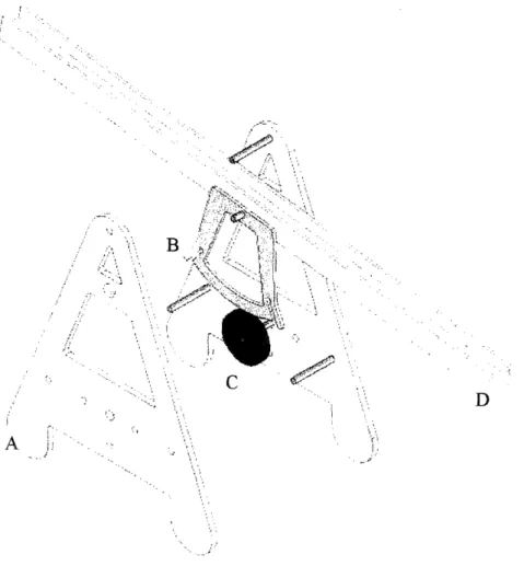
The mechanical design was developed with the objective of implementing the kit as part of a lab project in Feedback Systems (6.302). The kits therefore had to be simple, cheap, and easy to assemble. In the design selected, the primary parts of the structure are the frame, transmission mechanism and balance beam (Figure 3.1). The transmission
mechanism consists of a pulley on the motor shaft and a sector for gear reduction and
smaller motor requirement. In addition to being a simplistic design, the figure is also sleek, stylish and decorative.
C D
~~~~~~~A.~~~~~~~~~~~~~~~~~~~
'.
Figure 3.1. Solid Model of Apparatus. The primary parts of the structure are A) the Frame, B) the Sector, C) the Pulley, and D) the Beam.
3.1 Material Selection
To maintain low cost, materials were chosen for each specific component by considering durability, effectiveness, and cost. For the frame and sector, a low-cost polycarbonate was chosen. Polycarbonate is sufficiently stiff and lightweight compared to metal, and it
resists corrosion and oxidation. The pulley on the motor shaft was made from stock
Delrin, and the beam was made of basswood. The light weight and stiffness of basswood makes it a good choice to lower the moment of inertia while maintaining stiffness. Miscellaneous parts such as aluminum tubing and nylon bearings were used for bracing and assembling the apparatus. Table 3.1 shows a bill of materials per unit for a set of 50
kits. The total cost per kit is around $20, but does not include fabrication costs.
Table kit.
Material
Component
$/unit
Polycarbonate
Frame/sector
9.00
Delrin Motor pulley 0.40
Bass wood
Beam
2.15
1/4" x 2-1/4" bolts
Bracing
0.60
3/8" Al tube Bushing 0.33
1/4" Al tube Beam shaft 0.10
1/4" Nylon bearing Shaft bearing 0.52
Winchester Drive DC motor 5.00
1" stainless steel ball Ball 2.00
TOTAL: $20.10
3.1. Bill of Materials. The materials used to produce 50 units of the ball-on-beam
3.2 Manufacturing
Several manufacturing steps were taken to machine the raw materials. The construction
was done using a lathe and a water jet cutter. Simple tools such a band saw and drill
press were used to make minor cuts.
The first step in building the device was to cut the frame from a 1/4" polycarbonate sheet (Figure 3.2 a) and the sector from a 1/8" polycarbonate sheet (Figure 3.2 b). These
pieces were cut in the water jet cutter for repeatability, relatively clean cuts, and speed.
The tool paths for the parts were generated from a .dxf conversion of a SolidWorks solid
model. A sector and two frames were cut in 15 minutes.
/
i
/
Kt
[1
a;<
/-.,
\A9
0, .. X,
,!\
Figure 3.2a. Side frame made from
Figure 3.2b. Sector made from
polycarbonate. A part drawing is
polycarbonate. Flexures provide
generated in SolidWorks and then
preloading. Part drawing is generated in
machined in the water jet cutter. SolidWorks and part machined in water
jet cutter.
The pulley that is attached to the motor shaft was made of 2" Delrin rod. A 3/8" section
was cut from the stock and machined on the lathe. A 1/4" hole was drilled for the motor
shaft, and a 1/16" deep groove was cut in the center of the circumference to guide the transmission belt. After using the lathe, a hole was drilled from the outside groove to the
center hole to tap a setscrew.
Next, the beam was constructed using 2-foot-long basswood pieces. The dimensions of
the model were decided by considering the proportion of beam center height and beam
length. Because basswood is sold in 2-foot lengths, the beam was set at that length and
the other dimensions were determined with respect to that adjustment. The pivot was
placed 10 inches from the ground, and the overall height and width of the A-frame was set to 1 foot. The sector follows a designed developed by Stanford [6] with flexures for pre-tensioning the drive belt. The size of the sector was established by setting a gear
radius, the sector therefore had a 4" radius and an arbitrary 60°range. Once a beam that could support the conductive rail sensor was assembled, a 1/4" center hole was drilled, a 1/4" shaft was inserted, and the sector was attached.
Before final assembly, 2" bushings were cut from the 3/8" aluminum tube. At this point, the set-up was ready for assembly. The DC motor was fastened to the lower-middle portion of one of the frames, and the pulley was set on the motor shaft with a setscrew. Nylon bearings were then inserted into the guide holes for the beam shaft to rest. Next, the frames were put together with bolts, with the bushings separating them, the beam in
between, and the motor outside the structure. The final step in assembly was to connect
the pulley to the sector with a transmission belt. For this application, dental floss provided enough friction and tension. Figure 3.3 shows several fully assembled set-ups.
.- . . .. ,~~~~~~. :}
t0.;f.... ' ;w.- -'''
~~~~~~~~~~~
"~~' ,Figure 3.3. Fully Assembled Set-ups.
Chapter 4: Electronic Components
Substantial electrical work was necessary for the ball-balancer to function. The motor,
angle sensor, ball position sensor, and power electronics needed wiring as well as tuning.
The interface between the physical world and the digital world was a dSPACE controller
board with a Com port connection to a computer. This board accepted inputs from the
sensors and would output commands to the power amplifier, which in turn drove the
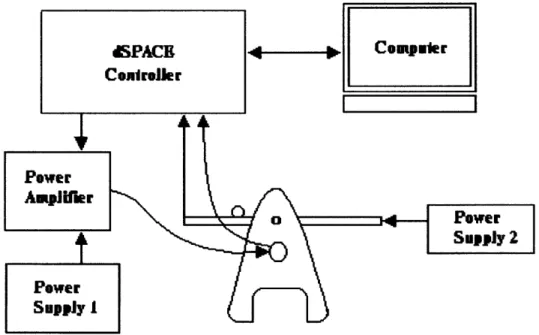
motor. Figure 4.1 shows the equipment involved in powering the system and how the
devices were connected.
Figure 4.1 Schematic Diagram of Ball-on-Beam System. A dSPACE controller
interfaced commands from a computer to output/input signals for the power amplifier and
motion sensors of the ball balancer. Power supply 1 supplied power to the power
amplifier while power supply 2 powered the ball position sensor.
4.1 DC Motor
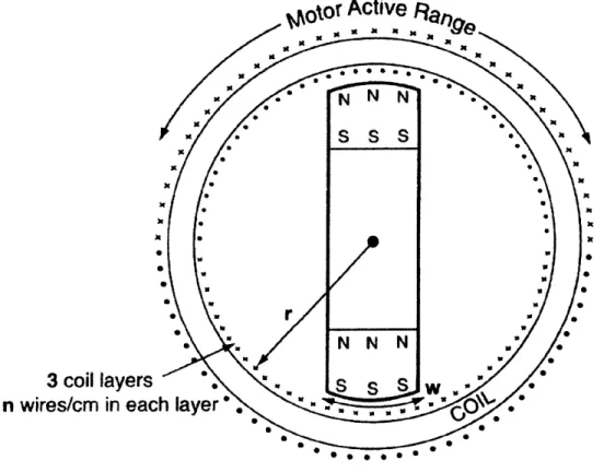
The DC motor used in this application was a Winchester disk drive motor (Appendix A)
that operates as a Lorenz force motor (Figure 4.2). As current, I, is driven through the
outer coils in the direction of length 1, a force, FL, is applied orthogonal to the magnetic
field, B, in the permanent magnets on the armature by the following law
By design of the armature, this force is always directed tangentially to the armature. It is
by this perpendicular force that a torque,
rm,is generated:
zm -=FrxFL, (4.2)
where r is the radius of the armature.
3 coil layers
n wires/cm in eac
- . *
Figure 4.2. Diagram of DC Motor. A permanent magnet armature has a magnetic field
that is perpendicular to the current running in the three layers of coils along the
circumference of the motor. The coils reverse polarity midway, thus limiting the rotation
of the motor shaft. Image taken from Mechatronics Lab Handout [7].
Because the coils reverse polarity to apply a force to both ends of the armature, the
operating range is limited to about 115°. This can be viewed as a hindrance in most other
applications, but because the beam is only expected to operate between + 10
°, this motor
is sufficient even with a 4:1 gear ratio. )
4.2 Angle Sensor
The angle sensor of the motor is an encoder mounted on the back of the Winchester
drive. The sensor operates on the A/B quadrature method [8]. Two leads connected to
the back of the motor case oscillate signal between
±0.35 V in a sinusoidal mode as the
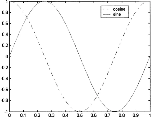
shaft is turned. The two leads are out of phase by a quarter cycle (i.e. sin kO and cos k0), which gives a reference point. As the position of the shaft changes, so does the signal of the two leads, and when either signal changes sign a count is given, depending on if the sine is leading or lagging. The count is increased if the sine is lagging and decreased if the sine is leading. There are 1100 cycles in one rotation (k = 360°/1100), or 4400 counts
per revolution. Therefore, the resolution of the encoder is 0.0818
°. Figure 4.3 represents
the concept of how A/B quadrature works.
1 0.8 0.6 0.4 0.2 0 -0.2 -0.4 -0.6 -0.8 -1 0 0.1 0.2 0.3 0.4 0.5 0.6 0.7 0.8 0.9 1
Figure 4.3. A/B Quadrature. Two signals, one sine (A), one cosine (B), vary as a function of angular position. As either of the two signals changes sign, a count is added
or subtracted depending on if the cosine is leading or lagging the sine.
The encoder counts were summed by the encoder channel in the dSPACE board.
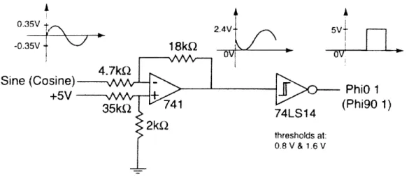
Because dSPACE only distinguishes digital signals, an analog circuit (Figure 4.4) was constructed to digitize the sine and cosine signals and center them about 1.2 V. A 741 op-amp was used to supply a 1.2 V biased voltage and increase the amplitude of the signal to 1.2 V. A 74LS 14 hex inverter with Schmitt trigger was used to relay an on/off signal at threshold voltages of 0.8 V and 1.6 V.
I- I X)" ' 'l ~ ' - -_ e rJ a~~~~~~~~-
~cosine
,
\
\
J~,
I~H
l \~~~~~~~~~~~~~~
'.'",,,~/
/, ~,~~~~~~~~~~~~~~~~ " \ N , y/",,I~~~~~~~~~
0.3 -0.3 Sine A I 1 PhiO 1 (Phi9 1)
Figure 4.4. Interface Circuit to Convert Encoder Signals. This circuit was used to
convert the analog encoder sinusoidal signals into digital square waves with 2.4 V
peak-to-peak amplitudes. Hysterisis induced by the Schmitt Trigger ensured that the signals
surpassed a threshold voltage before assigning a count. Image taken from Mechatronics
Lab Handout [7].
4.3 Ball Position Sensor
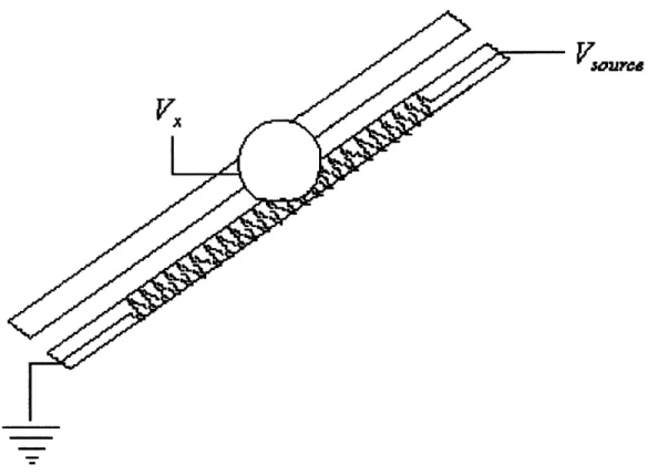
The ball position sensor used a linear potentiometer technique (Figure 4.5). Two
resistive rails, one 5 V from end to end, and the other floating to be used as a probe, used
a conductive steel ball as a wiper to transmit the voltage of the location of the ball, Vx,
along the rail to the other rail. Here the voltage divider rule is used as follows:
Vx = V source Rx
(43)
(4.3)where Vsource is 5 V, Rt is the total resistance of the rail, and RX is the resistance of the
section of rail from ground to the point where the ball makes contact. By knowing at
what voltage the ball is wiping a signal, the position of the ball can be correlated. This
position calculation assumes that the resistances of the rails are linear, which by
observation is true.
V5F
s~ouredVX
Figure 4.5. Linear Potentiometer Sensor. Two resistive rails were used to determine the
position of the ball along the beam. One rail carried a 5 V potential from end to end,
while the other rail used the ball as a wiper to measure the voltage correlating to the
Chapter 5: Control Design
The open-loop dynamics of the plant were discussed in Chapter 2. Equation 2.12 shows
that the system is fourth order with four free integrators, which means the uncontrolled
system is inherently unstable. To have the ball properly track a position command, a controller must be designed. The controller must be reliable and robust so as to not be easily excited into instability, and must also have good disturbance rejection. The
disturbance rejection should compensate for the torque that the ball mass applies as it
moves away from the center.
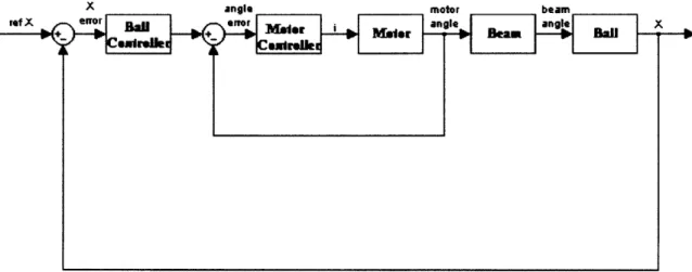
To begin, a block diagram for the closed loop system was constructed (Figure 5.1). In
this system there are only two sensors available: the motor angle sensor and the ball
position sensor. Therefore, there should be two closed loops, an inner motor loop and an
outer ball position loop. Another intermediary loop sensing the beam angle would be
beneficial in making the control and tuning of the system easier, but this loop is
unnecessary and was not implemented in this project.
X angle motor beam
ref A enor
[\
h iorlI--e
|i [
angle_[ ] angle[ XImrum I Lq I
Figure 5.1. Block Diagram of Closed Loop Ball-on-Beam System. An inner loop
controls the position of the motor, while the outer loop controls the position of the ball
along the beam.
5.1 Motor Controller
The design parameters of the controller adhere to the realistic performance expectations
of the system. For this application, a series of lead compensators were chosen to
counteract the abundance of open loop poles and improve transient response. An
i - P mmeir
position loop. Therefore, the realistic crossover frequency of the motor loop, Wom, was
arbitrarily chosen at about 25 Hz (158 radls). The lead compensator,
Gm/,
for the motor
was thus designated as
G_
(s+50)
(s + 500)
In addition to the lead compensator, an integrator with a 0.5 s time constant was
incorporated in cascade. The integrator transfer function,
G. _ (0.5s+1)
0.5s
combined with the motor lead compensator became the motor controller,
Gmc = (O.5s + 1) (s+50)
0.5s(s +
500)
(5.3)The bode plots of the lead compensator, integrator, the complete motor controller and the
open loop plant (Equation 2.10) are shown in Figure 5.2 and Figure 5.3. These plots
show the open loop characteristics of the controller and plant. Once the controller and
the motor are in cascade, the forward transmission transfer function for the motor
becomes
G.o = (0.5s+1) (s + 50)k,
.Ss(s + 500)Js2
(5.4) [, , , ., , . ... .... , .... 20 ~ E1 X.... .% ',% K / I') I1SiwlLS
,2-.
/' j 'i
,,./
s i1.,,, /- ' [I / / \ , _ ' 1 It to 1t xt~~~~~~~~'~ m Ft 0 ,,d , I[ ,,Figure 5.2. Model Bode Plots of Integrator and Lead Compensator.
(5.1)
II W so \ I ~ i -90 'NI I 1 , 1 I0 " 0 1I 0 - 1
tcUm) Frwe'y Atde)
Figure 5.3. Model Bode Plots of Motor Controller and Motor Forward Loop.
Equation 5.4 can be manipulated using block diagram algebra to calculate the motor
closed loop transfer function,
Gmcl =
(0.5s + 1) (s + 50)k,
0.5s(s + 500)Js2 + (0.5s + 1) (s +
50)k,
A step response of the motor closed loop transfer function is shown in Figure 5.4 and its corresponding Bode plot in Figure 5.5.
ilM e 10D - . I , . 8 . t-9 --(5.5) J Z f | -F_ ,, wH __ 4 , , , ,, ., I , , I .: -I \, '\ , r I -1-1 / I -bj , 0 1 -, -1 -I ._ ale
0.8 -) 0.6 0.4 2 0 Ui 0.05 0.1 0.15 0.2 0.25 0.:3 0.35 rme (sec:)
Figure 5.4. Theoretical Step Response of Closed Motor Loop.
0
-20
Ij G CR s -40 -60 45 a 0tD "o -45 -90 -1 35 -1 80 0.4 0.45 0.5 1:0 10 I10 10 Frequecy (radtsec)Figure 5.5. Model Closed Motor Loop Bode Plot. With an integrator and a lead
compensator, the motor loop became stable and had a gain of 0 at a bandwidth of 25 Hz. 1 0
5.2 Ball Controller
The transfer function in Equation 5.5 is the system that the ball controller acts upon. As
can be inferred in Figure 5.5, with the inner closed loop, the system becomes much more
manageable to control. Because the bandwidth of the ball-controlled system cannot
realistically be near 25 Hz, the ball dynamics will not interfere with the motor dynamics.
As was used in the motor loop, a lead compensator was implemented to control the ball
position. A 1 Hz (6 rad/s) bandwidth was desired to be achieved with the following lead controller:
Gbi
=(s+ 2)
(5.6)
(s + 20)
An integrator was not necessary in this loop because the integrator in the motor loop
diminished the ball error as well. The ball controller combined with the closed motor
loop gives the open loop transfer function of the ball position,
Gbol:G~
~g(0.5s
+ 1) (s + 50) (s + 2)k
t(57)
Gbol 2
s2 1
+
j
0[.
5s(s +
500
)Js2
+ (0.
5s + )
(s
+
50)k, ]
( + 20)
Figure 5.6 shows the Bode plot of the ball loop lead compensator and the forward path
transmission, and Figure 5.7 shows the closed loop Bode plot of the ball position. The
closed loop transfer function for the entire closed loop ball-on-beam system is
g(0.5s+l)
(s+50) (s+2
. (5.8)
G. =_
S21+ 2 a) [0.5s(s+500)Js2 +(O.5s+1) (s+50),](s+20)+g(O.5s+1) (s+50) (s+2)k, 9elLeCilmo~r 9l CRe lp as , An, ,,, ,~~~~~~/,,
, ., , .m, , ,, ,,, M5s a's Ima *"" 7~~~~~~~~~~~~~~R OdOWUM-:
Is~~~~~~~~~~~~~~~~~~~~~~~~~~l~~~~// I 5 7~ ~ ~
~
/ / I 1 :- 0 I I '] ;3 1 I ... Cl i ....- ,,r~':.... ... .... ... ,. ... £. 3 ) / \e . I' -i) . . .... . .~-
1
_I---I-'J_'
i _' 6 -\ _ X. - .. ... [ , I... 1 .' ' .'FUlm -10 -0 I) -40 !L
20
! IIII I I I I I I I I I I 1 I I I I I I I -I 13 ED EDU c" -90 -180 -;70 '10 10 10 10 Frequency (red/sec)Figure5.7. Model Closed Loop Bode Plot of Ball Position.
5.3 Control Implementation
With dSPACE, the closed loop controls are implemented with a Simulink model (Figure 5.8). Blocks for each controller are arranged and the proper signals are routed from input to output to close the loop in computer space. These signals are then mapped and
become variables in the graphical user interface, ControlDesk. Within this software, a control panel (Figure 5.9) can be designed using plotters, displays, slide bars, input boxes, etc., to view signals and vary parameters of the system.
D
ball rl
degrees integrator
Ground
Terminatorl
Figure 5.8. Simulink Model of Control Implementation. Blocks from the Simulink model library were used to construct the controllers and direct signals from input to
output.
: nOffl3 n I...
... . . .. . . .. . . . ... P.oset. Veue 0 200 40[ P:offset.Value 0.27000n . >~
~
~~~.
. .... . . _... 1l .. .... . . -. .' . P.lbeamGui -t 'I 0 E-3 . . . . .. . . . . . . . . . . . .. .5 -3 -1 1 3 5 3.0 0.1 o02 s G . . .. .. . .. . .. . . .. . . .. . . .. ,,:oem. .. . . ... F'740.= = ( --~~
. . . . .J I . . . . . . .. . . . .. . . .. . .. .. . .. . . . .. . . .. . .. . . . ... . .. . . . .. .. . . .. . . .I .. . . .. .. . . . . . . .. . . .. . . .. . . .. . . I . . . .. . ..~~~~.
. . .. . . .. . . .. . ... 0.3 04 o0s 0.6 07 0.8 0.9Figure 5.9. CntrolDesk Control Panel. In this graphical user interface, numerical displays and plotters were used to view different signals while slider bars, and input
boxes were used to adjust parameters of the control system.
o . . . . . . . -.- ... i I
...
.1 ...- ...
I, , .. ... _.. I I X * I ; l I I ; t I s 0, I,, . . . . I . . . I . . . . . . . . . . . . . . . . I . . . .Chapter 6: Test Results
A series of tests were conducted to verify the performance of the control design. Step
responses and bode plots were measured for the motor angle, and ball position. Bode
plots were measured dynamically using a Simulink block and Matlab script developed by Katherine Lilienkamp [9]. This dynamic analyzer provided a swept sine signal to drive an input and measure the output compared to an input designated anywhere along the
loop. The analyzer then calculated a transfer function and graphed the Bode plot.
6.1 Motor
The motor was designed to perform at a high bandwidth and diminish error. The expected behavior is described by the transfer function in Equation 5.4. The step
response of the ideal situation shown in Figure 5.4 and its Bode plot in Figure 5.5 can be compared to Figure 6.1 and Figure 6.2 respectively. The theoretical model and the
physical plant closely match. Whereas the idealized bandwidth was 25 Hz, the real
bandwidth was about 22 Hz. The damping also differed with the physical plant having
more natural damping than expected. Despite the subtle differences, the plant was tuned
well enough to resemble the designed model.
1 0.8 -E 0.6 0.4 0.2 0 0.05 0.1 0.15 0.2 Time (sec) 0.25
Figure 6.1. Actual Motor Step Response. The step response of the motor was measured
by commanding a step in the motor alone and measuring the resulting transient in angular
100 W 1: 10 0 10 102 Frequency (rad/sec) 0 -20 -40 -60 ~-613 t -100 OD
-120
ID 1 411 -140 -160 -180 10I 102 Frequency (radfsec)Figure 6.2. Measured Motor Bode Plot. The Bode plot was measured using a dynamic
analyzer that calculated the transfer function and plotted the corresponding Bode plot.
7
I I
'i I
6.2 Beam
The angle of the beam was not directly measured. Instead, the angle displacement of the
motor, when attached to the beam, was measured. The Bode plot in Figure 6.3 shows
how the motor angle in this coupled junction responded to varying frequencies. For low
frequencies, the beam closely followed the motor. However, after passing the first
resonance, anti-resonance occurred. At this frequency, excitation caused a small amplitude in the motor, but a large reaction in the beam. This physical plant feature
limited the dynamic capabilities, although, the ball was not designed to operate faster
than the first crossover frequency.
.-- --(5 -1 : 10 20 a CD cn a-EL -20 -40 -100 Frequency (rad/sec) Frequency (rad/sec)
Figure 6.3. Measured Bode Plot of Motor and Beam. This Bode plot was generated for
the closed loop performance of the motor when supporting the inertia of the beam. The
coupling between the motor and the beam caused an anti-resonance to occur after the first
resonance.
6.3 Ball
Having correctly closed the control loop of the motor, the closed loop of the ball was
expected to perform as predicted and have the ball achieve the designed parameters. The system gains had to be adjusted to attain adequate stiffness and damping. Once satisfied
with the adjustments, and once the ball was controlled at the center of the beam, a
disturbance was applied to the ball. As expected, the beam rotated to force the ball back
to its original position. If any oscillation was observed, the system was stable if the peak
displacement of an oscillation was less than the previous oscillation. This test showed
that the controller worked. Again, the system gain was adjusted to tune the oscillations
out. Eventually, what resulted was a critically damped step response. A step command
(Figure 6.4) could be ordered through the ControlDesk user interface. Essentially, the
ball could be balanced at any position along the beam. For small step commands, the ball
tracked the position quickly and without overshooting. For large step commands, the ball
tended to either overshoot and oscillated several times before coming to rest, or to
become unstable and lose system equilibrium. This defect can be attributed to the non-linearity in the system as well as the unreliability of the position sensor, which will be discussed in the next chapter. The non-linearity included the beam rotation angle dynamics, which was defined to be linear for small angles, and the contact of the ball on
the beam. For the bigger step commands the control effort became large enough to
command a significantly large beam rotation that initiated system instability.
0.305 0.3 O.2:~J
0.29
c
0.29
:20.285
oa
0.28 0.275 0.27 0.265 -1 0 1 2 3 4 5 6 7 8 9 Time (sec)Chapter 7: Sensor Issues
The biggest difficulties encountered in this project were introduced by the unreliability of
the ball position sensor. Because this sensor measured the system output, it was the most
critical component of the apparatus. If the position of the ball was not exactly known, the
position could not be precisely commanded. Noise that was introduced through this
sensor severely paralyzed the performance of the overall system. With the linear
potentiometer that was used in this set-up, the noise was a result of poor contact between
the resistive element and the conductive ball. Signal dropout occurred intermittently as
the ball rolled along the beam. For better signal transmission between the ball and the
contact sensor, the materials should be more carefully chosen. Steel tends to oxidize
easily and the oxide layer on the ball significantly increases the contact resistance. A beryllium-copper ball may be a better choice because the oxide of such a ball is also
conductive.
7.1 Tested Ball Position Sensors
Several options were explored before settling on the final ball position sensor design. Al
the sensors tested were some variation of a linear potentiometer. A voltage source was
conducted through one length of conductive rail while the other rail acted as a probe that
picked off the voltage through the ball in the same manner as a voltage divider.
The first material used as a rail was a train track as per the set-up used by Bob Pease [4].
Two N-gauge model railroad track segments about two-feet long were mounted onto the
beam. Current was driven through one rail to produce a voltage across the rail, while the
other rail sensed the position as the ball came in contact with the two rails. The first
problem with this set-up lay in the resistance of the railroad track. For a piece about
two-feet long, the resistance of the N-gauge track was about 0.5 ohms. This meant that a
large current was needed to produce any significant voltage. Even with 1 A of current
producing 0.5 V, the resolution was poor, and the signal was noisy. High contact resistance between the ball and the rail also caused large signal dropouts.
The next iterations of the rail design were primarily intended to reduce the power
requirements of the sensor. To meet this goal, the rail needed a higher resistance, which
could be accomplished through having a smaller cross-sectional area or choosing a more resistive material. Two lengths of 1/64" steel welding rod were affixed to the beam in
place of the train track and tested as a linear potentiometer sensor. The resistance across
a two-foot length of rod was about 2 ohms. This reduced the power consumption, but the
problem of poor contact resistance still remained. Just as with the train track, signal
fallout occurred even after cleaning ball and rail surfaces.
Another rail sensor material tested was a conductive plastic. Conductive polyolefin, with
a volume resistivity of about 3000 ohm/cm, was purchased from Westlake Plastics, and
This element provided excellent resolution with minimal power consumption. However,
the conductivity of this plastic was questionable. The surface of the plastic was
susceptible to scratches that would substantially increase the contact resistance, and
sufficient contact pressure was necessary for the ball to make good contact with the rails.
Under dynamic conditions, the ball was not guaranteed to have this pressure and the
signal often disappeared.
The final version of the sensor came from a packaged linear potentiometer with a
two-foot stroke. The resistive elements of Novotechnik TL600 linear potentiometers were
used as the senor for the ball position. The leads on which the wiper contacted were
coated with a layer of conductive material. The resistance across the length of the
element was about 20k ohms. Each element was positioned on the beam so as to create a
cradle for the ball to roll along where the point of contact was within the resistive portion of the element.
Of the sensors tested, the resistive element was the most effective. The resolution was
adequate and didn't require a high-power source. The contact was not quite so good, but
less signal fallout occurred than in the other sensors. Occasionally, some locations on the
rail registered a dead spot. This was caused by a spec of dirt or other foreign matter
resting on the rail. This problem was fixed by thoroughly cleaning the rail before use. In addition, applying a low-pass filter reduced signal fallout by adding a 0.1 jIF capacitor.
7.2 Alternate Ball Position Sensors
A linear potentiometer sensing technique was the only method tested, but other
techniques are possible and might have had better results. Some ideas involved contact sensors, while others involved non-contact sensors. These ideas included wound
nichrome wire, touch pads, acoustic transmission lines, ultrasonic transducers, and
infrared (IR) sensors.
Nickel-chromium (nichrome) wire is a highly resistive metal that is often used in heating coils. Because of nichrome's high resistivity, it is an attractive option as a sensor since it
would provide higher resolution and require less power than most metals of the same
size. In other classical implementations of the ball-on-beam problem, nichrome wire was
used [5]. Noise was a troublesome issue in these cases as well. However, if wound on a
plain or threaded dowel, the nichrome wire exposes less contact surface due to the
curvature around the dowel. Less contact surface means there will be higher contact
pressure and better conductivity from the ball to the sensor. The incremental pits also
limit the acceleration of the ball and make the ball easier to stop.
Touch pads that are commonly found on laptop computers and ATM touch screens
primarily work in one of three ways: resistive, capacitive, or acoustic wave changes. All touch pads are constructed in two layers, one layer monitoring changes in signals which
layer that stores electrical charge. As a person's finger comes in contact with the glass,
charge moves from the top layer to the person's finger. This location is measured by
calculating the relative difference in charge from circuits at different locations of the screen. Resistive touch pads have a conductive and resistive metallic layer that is held apart. As pressure is applied, the two layers come in contact. A computer calculates the change in electric field and its coordinates. Assuming the ball has enough mass to apply
enough pressure to a level touch pad, a feasible resistive touch pad beam sensor could be
designed. In this case, the ball would not have to be conductive. For a capacitive touch
pad, the ball would have to be conductive.
Based on the notion of the acoustic wave touch pad, an acoustic wave transmission line
sensor could be designed to determine the position of the ball along the beam. In this
design an actuator propagates a wave along some medium such as a metal rod and the
delayed reception is measured to determine if a disturbance was felt at a particular point
on the rod.
Another acoustic solution would be an ultrasonic range sensor. This transducer does not
require a solid medium to propagate. However, this sensor registers any foreign object
present in the proximity. Again, this sensor design does not need a conductive ball to
generate a position signal.
Lastly, a series of infrared sensors could be used to reveal the position of the ball on the
beam. Using this digital sensor, the resolution would depend on how closely together the
sensors can be arranged. The ball need not be conductive for this sensor design to
function properly. As the ball rolls past a sensor, the infrared beam is interrupted and the
feedback signal is sent to the controller.
Compared to the simplicity of the linear potentiometer, any of the sensors mentioned in
this section require a greater design effort, cost, and computation. Clearly, much more thought must occur to decide how to apply these sensing techniques. These designs will
require more extensive hardware and electronics, which would increase the cost of the
system. Along with affixing the sensor to the beam, the feedback signal(s) must also be
processed to supply the controller with the discrete position of the ball. For the purpose
of making kits available to students in feedback courses, the most cost-effective design is
the analog linear potentiometer described in this thesis.
7.3 Alternate Motor Angle Position Sensors
As described in Section 4.2, the motor angle was sensed by an encoder using quadrature counting. The encoder attached to the back of the motor was the most readily available
method to calculate the position of the motor and was therefore used. Although this
method was quite satisfactory, other methods could have been implemented. Two
solutions to this problem that are not digital are a rotary potentiometer and an
accelerometer.
A rotary potentiometer has a thin piece of resistive material on the hub of its case through
which a voltage is applied. As the shaft is rotated, a wiper moves along a resistive track.
The signal carried from the wiper is used to calculate the position of the shaft along the
rotary path. This measurement may add some resistance to the rotation of the motor
shaft, but the potentiometer's reading is reliable.
The other solution to measuring the angle of the motor is to use an accelerometer,
otherwise known as a gyro sensor. These devices detect the change in acceleration by measuring the change in electrical capacitance between two plates. These sensors tend to be less reliable for level measurements. The signal must be integrated twice and centered about an index point. This sensor is not DC-decoupled and introduces substantial noise into the signal.
Chapter 8: Future Work
Besides researching different sensors and determining which technique is most
advantageous for this application, there are other possible areas of improvement. The
mechanical design of the apparatus is an area that does not affect the performance of the
system, but it should be noted that a relocation of the center of gravity and a decrease of
overall dimensions could reduce material and cost. Two other main areas that could be redesigned are the controller and the transmission mechanism. The controller can be fine-tuned and even converted to analog control and the transmission mechanism can become more rigid or be eliminated.
8.1 Analog Control
The controller for this project was implemented in dSPACE using a Simulink model as mentioned in Section 5.3. The digital controller made implementation and adjustments
simpler. However, an analog controller would have made the control interface more
compact and easier to transport. Because the controllers are both lead controllers, the
circuitry could have been either active, with op-amps, or passive with only resistors and capacitors. Figure 8.1 shows a sample controller circuit that could be used to implement
a lead controller as in Equation 5.6.
CI
R3 CI
iLnpul RZ oulpulRI
R2
(a) inpLutouilPl
RI
(b)Figure 8.1. Analog Lead Controller. An analog lead controller could be implemented with either a passive circuit (a), or active circuit (b).
8.2 Transmission Redesign
Whereas the controller design can be adjusted to improve transient responses, the plant
ultimately determines its limitations. Once the plant has been built, it can no longer be adjusted easily. A simple mechanical design can help improve the dynamic capability of the control system. To have a higher bandwidth and crossover frequency, either the
inertia of the plant needs to decrease or the transmission mechanism needs to become
stiffer. One way to make the transmission stiffer is to use a stiffer transmission belt than dental floss. Another way is to design stiffer flexures in the gear-reducing sector. The best way would be to completely remove the transmission and make the beam a direct drive. The initial reason for including a transmission was to provide mechanical
advantage and enable the available motor to power the movements of the beam.
Otherwise, as a direct drive, the given motor would not have been able to effectively
manipulate the inertia ofthe beam. With a direct drive, the motor needs to be able to supply enough torque to support the mass of the ball at whatever distance away from the center that is desired. Using the current frame design, the motor and beam would also need additional support because the center of mass would be higher than its midpoint.
Alternatively, the location of the beam could be lowered to move the center of gravity
closer to the bottom of the structure.
Chapter 9: Conclusion
The ball-on-beam kit that was designed is simple, easy to assemble, and cost effective. It is also visually appealing and attractive as a decorative souvenir of a class project. Using this kit as a pedagogical instrument to teach feedback systems benefits both the instructor
and the students. First, the kits are low cost, so there is not a big budget concern for the
instructor. Second, this problem is interesting enough to capture the interest of most
students. The ball-on-beam problem is a good opportunity to apply classical control. Students in the feedback systems class in the electrical engineering department enjoyed
designing controllers and the ball position sensor for the system. Most groups were
successful in implementing their controller and sensor designs. There was a range of system successes, but all students learned valuable lessons.
The controller described in this thesis worked as designed. The main factor that troubled
the controller was the poor quality of signal received from the ball position sensor. The
noise, which was large for the first three sensors tested, saturated the amplifier because the derivative in the lead controller amplified the noise signal. Once the sensor was
improved and the noise reduced, the controller worked as expected.
The most difficult part was indeed the ball position sensor design. This aspect of the
project could be researched further. The ideas in Section 7.2 would be a starting point for possible sensor designs, and from those ideas, others would develop. In completing this
project, it was often frustrating to realize that without a proper position measurement,
control was impossible. A significant amount of time was spent testing different sensors
and debugging them. After the initial mechanical and controller designs were done, attention was heavily focused on the design and success of the ball position sensor.
This project was a good opportunity to create hardware and implement a controller. The
idiosyncrasies of real plants were revealed through variation and experimentation. These
details were noted and can now be expected in similar cases. A sense of enthusiasm was
developed and a passion to continue researching the area of controls was generated in the
author.
Acknowledgments
I would like to thank Professor Trumper for providing me guidance throughout the entire
project and helping me debug the system. I would also like to thank Dr. Lundberg and Katie Lilienkamp for suggesting this project. Dr. Lundberg implemented this project as the final assignment in Feedback Systems (6.302) and helped me write a paper for a conference in July 2004. I thank Katie for getting me started with ideas and helping me
get acquainted with dSPACE and Simulink models. Thanks goes to Rick Montesanti for
discussing with me at length about different aspects of my design and helped me better
understand what was occurring in the system. The rest of the group in the Precision
Motion Control Lab also discussed my project with me. Special thanks goes to Darcy
Kelly for providing moral support when it seemed like my project would never work and
for making me dinner to help me forget about school work all together. Another special
thanks goes to Noosheen Khalil-Naji for distracting me from my thesis writing when I
was progressing and for forcing me to write when I had writer's block. Her moral
support and encouragement helped me to work hard and complete this project. Last, but
not least, thanks to Stacia Swanson for editing this document.
Appendix A: Winchester Disk Drive Motor
Specifications
These motor characteristics were converted to metric units from the English units used in
the Litton Encoder Division data sheet for the Winchester Disk Drive Motor. The
original specification sheet is on the subsequent page.
Value 3.885 x 10- 2 3.885 x 10⁻² 3.7
2.02 x
10-2 9.18 x 10-26.07 x
10-2 1.2 x 10⁻⁵ 4.45 x 10.4Units
Nm/A
V/rad/s
ohmsNm/l[W
Nm
Nm
Nms2Nm/rad/s
Description
torque sensitivity
back EMF constant
armature resistance
motor constant
peak torque
continuous torque
rotor inertia
viscous dampingConstant
kt km Tp Tc Jr B1.0 DEISCRIPTION:
Tis
specificaLion
detiints
an encoder
to be
coupledto
a
illited Angle
rt,.shless DC Motor in a 5k
Winchester
Disk D)rive
The ecoder
is to provide tilhree
output
signals.
Oe
outpult is
Channel
A; secoid is Channel
; and the third
is an Index or Reference Pulse. Channels A and B exhibit
a relationship
such that A is a Sine fnction.
while B
performs the Cosine function.
The outputs from the Sine and the Cosine are analog
and represent the actual resolution on the code disk.
Any reference of CW
or CCW
rotation in te following is
assumed to be seen from the encoder side of the motor.
2.0 MECHANICAL CHARACTERIlSTlCS:
2.1 MOTOR/ENCODER
DIMENSIONS
1.545"
AX (REF FG
1)SHT 5
2.1.1 MOTOR 1.006" MAX
2.1.2
ENC(GDER
.539" MAX
2.1. 3
SH
'tjD
Do
'V '
2500
20
-. 0005"
.o0o"
2 .1.4 D'T LENCh' .82 MAX
(LOAD SIDE)
2.2 COMMt/I[UB INERTIA 200 (106) OZ-IN SEC2 MAX
2.3 RESOLUTION 1100 CYCLES/REV
2.3.: IN)EX I ?V!"SE/;,EV 5 CYCV!.t' LONC
2.4 SPEED 600 RPM MAX
2,.5 ACCELERATION 6000 RAD/SEC2 MAX
3.0 MOTOR CHARACTERISTICS @200C:
+ 0
3.1 ECURSION ANCLE
60
°O
3.2 TORQUE SENSITIVITY
5.5 OZ-IN/AMP
Kt
3.3 BACK EMF CONSTANT .0388 VOLTS/RADS/SEC Ke
3.4 RESISTANCF. 3. 7_ R
3.5 MOTOR CONSTANT 2.86 OZ-IN/WATTS Km
3.6 PEAK TORQUE 13 0Z-IN Tp
3.7 CONTINUOUS TORQUE 8.6 OZ-IN Tc
3.8
ROTOR
INERTIA 1.7 (10- 3) OZ-IN-SEC 2 Jr3.9 VISCOUS DAMPING .063 OZ-IN/RAD/SEC D
References
[1] Product Information Sheet R2-1, Rotary Ball & Beam Experiment, Quanser Inc.,
Markham, ON, Canada.
[2] R. Hirsch, Shandor Motion Systems, "Ball on Beam Instructional System," Shandor
Motion Systems, 1999.
[3] K. C. Craig, J. A. de Marchi, "Mechatronic System Design at Rensselaer," in 1995
International Conference on Recent Advances in Mechatronics, Istanbul, Turkey,
August 14-16.
[4] R. A. Pease, "What's All This Ball-On-Beam-Balancing Stuff, Anyhow," Electronic Design Analog Applications, p. 50-52, November 20, 1995.
[5] G. J. Kenwood, "Modem control of the classic ball and beam problem," B.S. thesis,
Massachusetts Institute of Technology, Cambridge, MA, 1982.
[6] C. Richard, A. M. Okamura, M. R. Cutkosky, "Getting a Feel for Dynamics: Using Haptic Interface Kits for Teaching Dynamics and Controls," 1997 ASME IMECE 6th Annual Symposium on Haptic Interfaces, Dallas, TX, Nov. 15-21.
[7] "Laboratory Assignment 4: Brushless Motor Control," lab handout for 2.737
Mechatronics, Department of Mechanical Engineering, Massachusetts Institute of
Technology, Spring 1999.
[8] Gurley Precision Instruments, "Understanding Quadrature," 1998,
http://www.gpi-encoders. com/Understanding_Quadrature.pdf.
[9] K. A. Lilienkamp, "A simulink-driven dynamic signal analyzer," B.S. thesis,


![[PDF] Cours de Perl : introduction generale sur les principaux savoir-faire du langage perl | Cours perl](data:image/gif;base64,R0lGODlhAQABAIAAAP///wAAACH5BAEAAAAALAAAAAABAAEAAAICRAEAOw==)