[It] showed how to differentiate parameters under the integral sign – it’s a certain operation

KEITH CONRAD

I had learned to do integrals by various methods shown in a book that my high school physics teacher Mr. Bader had given me. [It] showed how to differentiate parameters under the integral sign – it’s a certain operation. It turns out that’s not taught very much in the universities; they don’t emphasize it. But I caught on how to use that method, and I used that one damn tool again and again. [If] guys at MIT or Princeton had trouble doing a certain integral, [then] I come along and try differentiating under the integral sign, and often it worked. So I got a great reputation for doing integrals, only because my box of tools was different from everybody else’s, and they had tried all their tools on it before giving the problem

to me.¹ Richard Feynman [5, pp. 71–72]²

1. Introduction

The method of differentiation under the integral sign, due to Leibniz in 1697 [4], concerns integrals depending on a parameter, such as R1

0 x²e^−txdx. Here t is the extra parameter. (Since x is the variable of integration, x isnot a parameter.) In general, we might write such an integral as (1.1)

Z b a

f(x, t) dx,

wheref(x, t) is a function of two variables likef(x, t) =x²e^−tx. Example 1.1. Letf(x, t) = (2x+t³)². Then

Z 1 0

f(x, t) dx= Z 1

0

(2x+t³)²dx. An anti-derivative of (2x+t³)² with respect to x is ¹₆(2x+t³)³, so

Z 1 0

(2x+t³)²dx= (2x+t³)³ 6

x=1 x=0

= (2 +t³)³−t⁹

6 = 4

3 + 2t³+t⁶.

This answer is a function of t, which makes sense since the integrand depends ont. We integrate overx and are left with something that depends only on t, not x.

An integral like Rb

af(x, t) dx is a function of t, so we can ask about its t-derivative, assuming that f(x, t) is nicely behaved. The rule, called differentiation under the integral sign, is that the t-derivative of the integral off(x, t) is the integral of the t-derivative off(x, t):

(1.2) d

dt Z b

a

f(x, t) dx= Z b

a

∂

∂tf(x, t) dx.

1See https://scientistseessquirrel.wordpress.com/2016/02/09/do-biology-students-need-calculus/ for a similar story with integration by parts in the first footnote.

2Just before this quote, Feynman wrote “One thing I never did learn was contour integration.” Perhaps he meant that he never felt he learned itwell, since he did know it. See [6, Lect. 14, 15, 17, 19], [7, p. 92], and [8, pp. 47–49].

A challenge he gave in [5, p. 176] suggests he didn’t like contour integration.

1

If you are used to thinking mostly about functions with one variable, not two, keep in mind that (1.2) involves integrals and derivatives with respect to separatevariables: integration with respect tox and differentiation with respect tot.

Example 1.2. We saw in Example1.1that R1

0(2x+t³)²dx= 4/3 + 2t³+t⁶, whoset-derivative is 6t²+ 6t⁵. According to (1.2), we can also compute the t-derivative of the integral like this:

d dt

Z 1 0

(2x+t³)²dx = Z 1

0

∂

∂t(2x+t³)²dx

= Z 1

0

2(2x+t³)(3t²) dx

= Z 1

0

(12t²x+ 6t⁵) dx

= 6t²x²+ 6t⁵x

x=1 x=0

= 6t²+ 6t⁵. The answer agrees with our first, more direct, calculation.

We will apply (1.2) to many examples of integrals, in Section12 we will discuss the justification of this method in our examples, and then we’ll give some more examples.

2. Euler’s factorial integral in a new light For integers n≥0, Euler’s integral formula forn! is

(2.1)

Z ∞ 0

xⁿe^−xdx=n!,

which can be obtained by repeated integration by parts starting from the formula (2.2)

Z ∞ 0

e^−xdx= 1

whenn= 0. Now we are going to derive Euler’s formula in another way, by repeated differentiation after introducing a parameter tinto (2.2).

Fort >0, let x=tu. Then dx=tduand (2.2) becomes Z ∞

0

te^−tudu= 1.

Dividing byt and writingu asx (why is this not a problem?), we get (2.3)

Z ∞ 0

e^−txdx= 1 t.

This is a parametric form of (2.2), where both sides are now functions oft. We needt >0 in order thate^−tx is integrable over the region x≥0.

Now we bring in differentiation under the integral sign. Differentiate both sides of (2.3) with respect tot, using (1.2) to treat the left side. We obtain

Z ∞ 0

−xe^−txdx=−1 t²,

so (2.4)

Z ∞ 0

xe^−txdx= 1 t².

Differentiate both sides of (2.4) with respect to t, again using (1.2) to handle the left side. We get Z ∞

0

−x²e^−txdx=−2 t³. Taking out the sign on both sides,

(2.5)

Z ∞ 0

x²e^−txdx= 2 t³.

If we continue to differentiate each new equation with respect tot a few more times, we obtain Z ∞

0

x³e^−txdx= 6 t⁴, Z ∞

0

x⁴e^−txdx= 24 t⁵,

and Z ∞

0

x⁵e^−txdx= 120 t⁶ . Do you see the pattern? It is

(2.6)

Z ∞ 0

xⁿe^−txdx= n!

tⁿ⁺¹.

We have used the presence of the extra variable t to get these equations by repeatedly applying d/dt. Now specialize tto 1 in (2.6). We obtain

Z ∞ 0

xⁿe^−xdx=n!, which is our old friend (2.1). Voil´a!

The idea that made this work is introducing a parametert, using calculus ont, and then setting t to a particular value so it disappears from the final formula. In other words, sometimesto solve a problem it is useful to solve a more general problem. Compare (2.1) to (2.6).

3. A damped sine integral We are going to use differentiation under the integral sign to prove

Z ∞ 0

e^−txsinx

x dx= π

2 −arctant fort >0.

Call this integralF(t) and setf(x, t) =e^−tx(sinx)/x, so (∂/∂t)f(x, t) =−e^−txsinx. Then F⁰(t) =−

Z ∞ 0

e^−tx(sinx) dx.

The integrand e^−txsinx, as a function ofx, can be integrated by parts:

Z

e^axsinxdx= (asinx−cosx) 1 +a² e^ax.

Applying this witha=−t and turning the indefinite integral into a definite integral, F⁰(t) =−

Z ∞ 0

e^−tx(sinx) dx= (tsinx+ cosx) 1 +t² e^−tx

x=∞

x=0

.

Asx→ ∞,tsinx+ cosx oscillates a lot, but in a bounded way (since sinxand cosxare bounded functions), while the terme^−tx decays exponentially to 0 since t >0. So the value at x=∞ is 0.

Therefore

F⁰(t) =− Z ∞

0

e^−tx(sinx) dx=− 1 1 +t².

We know an explicit antiderivative of 1/(1 + t²), namely arctant. Since F(t) has the same t-derivative as −arctant, they differ by a constant: for some number C,

(3.1)

Z ∞ 0

e^−txsinx

x dx=−arctant+C fort >0.

We’ve computed the integral, up to an additive constant, without finding an antiderivative of e^−tx(sinx)/x.

To compute C in (3.1), let t → ∞ on both sides. Since |(sinx)/x| ≤ 1, the absolute value of the integral on the left is bounded from above by R∞

0 e^−txdx = 1/t, so the integral on the left in (3.1) tends to 0 as t → ∞. Since arctant → π/2 as t → ∞, equation (3.1) as t → ∞ becomes 0 =−^π₂ +C, soC=π/2. Feeding this back into (3.1),

(3.2)

Z ∞ 0

e^−txsinx

x dx= π

2 −arctant fort >0.

If we lett→0⁺ in (3.2), this equation suggests that (3.3)

Z ∞ 0

sinx

x dx= π 2,

which is true and it is important in signal processing and Fourier analysis. It is a delicate matter to derive (3.3) from (3.2) since the integral in (3.3) is not absolutely convergent. Details are provided in an appendix.

4. The Gaussian integral The improper integral formula

(4.1)

Z ∞

−∞

e^−x2/2dx=√ 2π

is fundamental to probability theory and Fourier analysis. The function ^√1

2πe^−x2/2 is called a Gaussian, and (4.1) says the integral of the Gaussian over the whole real line is 1.

The physicist Lord Kelvin (after whom the Kelvin temperature scale is named) once wrote (4.1) on the board in a class and said “A mathematician is one to whom that [pointing at the formula] is as obvious as twice two makes four is to you.” We will prove (4.1) using differentiation under the integral sign. The method will not make (4.1) as obvious as 2·2 = 4. If you take further courses you may learn more natural derivations of (4.1) so that the result really does become obvious. For now, just try to follow the argument here step-by-step.

We are going to aim not at (4.1), but at an equivalent formula over the range x≥0:

(4.2)

Z ∞ 0

e^−x2/2dx=

√ 2π

2 =

rπ 2.

Call the integral on the left I.

Fort∈R, set

F(t) = Z ∞

0

e^{−t2(1+x2)/2} 1 +x² dx.

Then F(0) =R∞

0 dx/(1 +x²) =π/2 andF(∞) = 0. Differentiating under the integral sign, F⁰(t) =

Z ∞ 0

−te^{−t2(1+x2)/2}dx=−te^−t2/2 Z ∞

0

e^−(tx)2/2dx.

Make the substitutiony =tx, with dy=tdx, so F⁰(t) =−e^−t2/2

Z ∞ 0

e^−y2/2dy =−Ie^−t2/2.

Forb >0, integrate both sides from 0 tob and use the Fundamental Theorem of Calculus:

Z b 0

F⁰(t) dt=−I Z b

0

e^−t2/2dt=⇒F(b)−F(0) =−I Z b

0

e^−t2/2dt.

Lettingb→ ∞,

0−π

2 =−I²=⇒I²= π

2 =⇒I = rπ

2.

I learned this from Michael Rozman [12], who modified an idea on a Math Stackexchange question [3], and in a slightly less elegant form it appeared much earlier in [15].

5. Higher moments of the Gaussian For every integer n≥0 we want to compute a formula for

(5.1)

Z ∞

−∞

xⁿe^−x2/2dx.

(Integrals of the typeR

xⁿf(x) dxforn= 0,1,2, . . . are called themomentsoff(x), so (5.1) is the n-th moment of the Gaussian.) When n is odd, (5.1) vanishes since xⁿe^−x2/2 is an odd function.

What if n= 0,2,4, . . . is even?

The first case, n= 0, is the Gaussian integral (4.1):

(5.2)

Z ∞

−∞

e^−x2/2dx=√ 2π.

To get formulas for (5.1) whenn6= 0, we follow the same strategy as our treatment of the factorial integral in Section 2: stick a t into the exponent of e^−x2/2 and then differentiate repeatedly with respect tot.

Fort >0, replacingx with√

tx in (5.2) gives (5.3)

Z ∞

−∞

e^−tx2/2dx=

√2π

√t .

Differentiate both sides of (5.3) with respect tot, using differentiation under the integral sign on the left:

Z ∞

−∞

−x²

2 e^−tx2/2dx=−

√2π 2t^3/2, so

(5.4)

Z ∞

−∞

x²e^−tx2/2dx=

√ 2π t^3/2 .

Differentiate both sides of (5.4) with respect to t. After removing a common factor of −1/2 on both sides, we get

(5.5)

Z ∞

−∞

x⁴e^−tx2/2dx= 3√ 2π t^5/2 .

Differentiating both sides of (5.5) with respect tota few more times, we get Z ∞

−∞

x⁶e^−tx2/2dx= 3·5√ 2π t^7/2 , Z ∞

−∞

x⁸e^−tx2/2dx= 3·5·7√ 2π t^9/2 , and

Z ∞

−∞

x¹⁰e^−tx2/2dx= 3·5·7·9√ 2π t^11/2 . Quite generally, when nis even

Z ∞

−∞

xⁿe^−tx2/2dx= 1·3·5· · ·(n−1) t^(n+1)/2

√ 2π,

where the numerator is the product of the positive odd integers from 1 ton−1 (understood to be the empty product 1 when n= 0).

In particular, takingt= 1 we have computed (5.1):

Z ∞

−∞

xⁿe^−x2/2dx= 1·3·5· · ·(n−1)

√ 2π.

As an application of (5.4), we now compute (¹₂)! :=R∞

0 x^1/2e^−xdx, where the notation (¹₂)! and its definition are inspired by Euler’s integral formula (2.1) for n! when nis a nonnegative integer.

Using the substitutionu=x^1/2 inR∞

0 x^1/2e^−xdx, we have 1

2

! = Z ∞

0

x^1/2e^−xdx

= Z ∞

0

ue^−u2(2u) du

= 2 Z ∞

0

u²e^−u2du

= Z ∞

−∞

u²e^−u2du

=

√2π

2^3/2 by (5.4) at t= 2

=

√π 2 .

6. A cosine transform of the Gaussian We are going to compute

F(t) = Z ∞

0

cos(tx)e^−x2/2dx

by looking at its t-derivative:

(6.1) F⁰(t) =

Z ∞ 0

−xsin(tx)e^−x2/2dx.

This isgood from the viewpoint of integration by parts since −xe^−x2/2 is the derivative ofe^−x2/2. So we apply integration by parts to (6.1):

u= sin(tx), dv=−xe^−x2dx and

du=tcos(tx) dx, v=e^−x2/2. Then

F⁰(t) = Z ∞

0

udv

= uv

∞ 0

− Z ∞

0

vdu

= sin(tx) e^x2/2

x=∞

x=0

−t Z ∞

0

cos(tx)e^−x2/2dx

= sin(tx) e^x2/2

x=∞

x=0

−tF(t).

Asx→ ∞,e^x2/2 blows up while sin(tx) stays bounded, so sin(tx)/e^x2/2 goes to 0. Therefore F⁰(t) =−tF(t).

Weknow the solutions to this differential equation: constant multiples ofe^−t2/2. So Z ∞

0

cos(tx)e^−x2/2dx=Ce^−t2/2 for some constant C. To findC, set t= 0. The left side is R∞

0 e^−x2/2dx, which is p

π/2 by (4.2).

The right side is C. Thus C=p

π/2, so we are done: for all real t, Z ∞

0

cos(tx)e^−x2/2dx= rπ

2e^−t2/2. Remark 6.1. If we want to computeG(t) =R∞

0 sin(tx)e^−x2/2dx, with sin(tx) in place of cos(tx), then in place ofF⁰(t) =−tF(t) we haveG⁰(t) = 1−tG(t), andG(0) = 0. From the differential equa- tion, (e^t2/2G(t))⁰ =e^t2/2, so G(t) =e^−t2/2Rt

0 e^x2/2dx. So while R∞

0 cos(tx)e^−x2/2dx =p_π

2e^−t2/2, the integral R∞

0 sin(tx)e^−x2/2dx is impossible to express in terms of elementary functions.

7. The Gaussian times a logarithm We will compute

Z ∞ 0

(logx)e^−x2dx.

Integrability at∞follows from rapid decay ofe^−x2 at∞, and integrability nearx= 0 follows from the integrand there being nearly logx, which is integrable on [0,1], so the integral makes sense.

(This example was brought to my attention by Harald Helfgott.)

We already know R∞

0 e^−x2dx=√

π/2, but how do we find the integral when a factor of logx is inserted into the integrand? Replacing x with√

x in the integral, (7.1)

Z ∞ 0

(logx)e^−x2dx= 1 4

Z ∞ 0

logx

√x e^−xdx.

To compute this last integral, the key idea is that (d/dt)(x^t) = x^tlogx, so we get a factor of logx in an integral after differentiation under the integral sign if the integrand has an exponential parameter: for t >−1 set

F(t) = Z ∞

0

x^te^−xdx.

(This is integrable for x near 0 since for small x, x^te^−x ≈ x^t, which is integrable near 0 since t >−1.) Differentiating both sides with respect to t,

F⁰(t) = Z ∞

0

x^t(logx)e^−xdx, so (7.1) tells us the number we are interested in is F⁰(−1/2)/4.

The functionF(t) is well-known under a different name: fors >0, the Γ-function at sis defined by

Γ(s) = Z ∞

0

x^s−1e^−xdx,

so Γ(s) =F(s−1). Therefore Γ⁰(s) =F⁰(s−1), soF⁰(−1/2)/4 = Γ⁰(1/2)/4. For the rest of this section we work out a formula for Γ⁰(1/2)/4 using properties of the Γ-function; there is no more differentiation under the integral sign.

We need two standard identities for the Γ-function:

(7.2) Γ(s+ 1) =sΓ(s), Γ(s)Γ

s+1

2

= 2^1−2s√

πΓ(2s).

The first identity follows from integration by parts. Since Γ(1) =R∞

0 e^−xdx= 1, the first identity implies Γ(n) = (n−1)! for every positive integer n. The second identity, called the duplication formula, is subtle. For example, ats= 1/2 it says Γ(1/2) =√

π. A proof of the duplication formula can be found in many complex analysis textbooks. (The integral defining Γ(s) makes sense not just for real s >0, but also for complex swith Re(s) >0, and the Γ-function is usually regarded as a function of a complex, rather than real, variable.)

Differentiating the first identity in (7.2),

(7.3) Γ⁰(s+ 1) =sΓ⁰(s) + Γ(s),

so ats= 1/2 (7.4) Γ⁰

3 2

= 1 2Γ⁰

1 2

+ Γ

1 2

= 1 2Γ⁰

1 2

+√

π =⇒Γ⁰ 1

2

= 2

Γ⁰ 3

2

−√ π

.

Differentiating the second identity in (7.2), (7.5) Γ(s)Γ⁰

s+1

2

+ Γ⁰(s)Γ

s+1 2

= 2^1−2s(−log 4)√

πΓ(2s) + 2^1−2s√

π2Γ⁰(2s).

Settings= 1 here and using Γ(1) = Γ(2) = 1,

(7.6) Γ⁰

3 2

+ Γ⁰(1)Γ 3

2

= (−log 2)√ π+√

πΓ⁰(2).

We compute Γ(3/2) by the first identity in (7.2) at s = 1/2: Γ(3/2) = (1/2)Γ(1/2) = √

π/2 (we already computed this at the end of Section 5). We compute Γ⁰(2) by (7.3) at s = 1: Γ⁰(2) = Γ⁰(1) + 1. Thus (7.6) says

Γ⁰ 3

2

+ Γ⁰(1)

√π

2 = (−log 2)√ π+√

π(Γ⁰(1) + 1) =⇒Γ⁰ 3

2

=√ π

−log 2 + Γ⁰(1) 2

+√

π.

Feeding this formula for Γ⁰(3/2) into (7.4), Γ⁰

1 2

=√

π(−2 log 2 + Γ⁰(1)).

It turns out that Γ⁰(1) =−γ, where γ ≈.577 is Euler’s constant. Thus, at last, Z ∞

0

(logx)e^−x2dx= Γ⁰(1/2)

4 =−

√π

4 (2 log 2 +γ).

8. Logs in the denominator, part I Consider the following integral over [0,1], wheret >0:

Z 1 0

x^t−1 logx dx.

Since 1/logx → 0 as x → 0⁺, the integrand vanishes at x = 0. As x → 1⁻, (x^t−1)/logx → t.

Therefore whentis fixed the integrand is a continuous function ofx on [0,1], so the integral is not an improper integral.

The t-derivative of this integral is Z 1

0

x^tlogx logx dx=

Z 1 0

x^tdx= 1 t+ 1, which we recognize as thet-derivative of log(t+ 1). Therefore

Z 1 0

x^t−1

logx dx= log(t+ 1) +C

for some C. To findC, let t→0⁺. On the right side, log(1 +t) tends to 0. On the left side, the integrand tends to 0: |(x^t−1)/logx|=|(e^tlogx−1)/logx| ≤tbecause |e^a−1| ≤ |a|whena≤0.

Therefore the integral on the left tends to 0 as t→0⁺. So C= 0, which implies (8.1)

Z 1 0

x^t−1

logx dx= log(t+ 1)

for allt >0, and it’s obviously also true fort= 0. Another way to compute this integral is to write x^t=e^tlogx as a power series and integrate term by term, which is valid for−1< t <1.

Under the change of variablesx=e^−y, (8.1) becomes (8.2)

Z ∞ 0

e^−y−e^−(t+1)y dy

y = log(t+ 1).

9. Logs in the denominator, part II We now consider the integral

F(t) = Z ∞

2

dx x^tlogx for t > 1. The integral converges by comparison with R∞

2 dx/x^t. We know that “at t = 1” the integral diverges to∞:

Z ∞ 2

dx

xlogx = lim

b→∞

Z b 2

dx xlogx

= lim

b→∞log logx

b 2

= lim

b→∞log logb−log log 2

= ∞.

So we expect that ast→1⁺,F(t) should blow up. But howdoes it blow up? By analyzingF⁰(t) and then integrating back, we are going to showF(t) behaves essentially like−log(t−1) ast→1⁺.

Using differentiation under the integral sign, fort >1 F⁰(t) =

Z ∞ 2

∂

∂t 1

x^tlogx

dx

= Z ∞

2

x^−t(−logx) logx dx

= −

Z ∞ 2

dx x^t

= − x^−t+1

−t+ 1

x=∞

x=2

= 2^1−t 1−t.

We want to bound this derivative from above and below whent >1. Then we will integrate to get bounds on the size ofF(t).

Fort >1, the difference 1−tis negative, so 2^1−t<1. Dividing both sides of this by 1−t, which is negative, reverses the sense of the inequality and gives

2^1−t 1−t > 1

1−t.

This is a lower bound on F⁰(t). To get an upper bound on F⁰(t), we want to use a lower bound on 2^1−t. Sincee^a≥a+ 1 for alla (the graph ofy =e^x lies on or above its tangent line atx = 0, which isy=x+ 1),

2^x=e^{xlog 2}≥(log 2)x+ 1 for all x. Takingx= 1−t,

(9.1) 2^1−t≥(log 2)(1−t) + 1.

When t >1, 1−tis negative, so dividing (9.1) by 1−treverses the sense of the inequality:

2^1−t

1−t ≤log 2 + 1 1−t.

This is an upper bound on F⁰(t). Putting the upper and lower bounds on F⁰(t) together,

(9.2) 1

1−t < F⁰(t)≤log 2 + 1 1−t for all t >1.

We are concerned with the behavior ofF(t) ast→1⁺. Let’s integrate (9.2) from ato 2, where 1< a <2:

Z ₂

a

dt 1−t <

Z ₂

a

F⁰(t) dt≤ Z ₂

a

log 2 + 1 1−t

dt.

Using the Fundamental Theorem of Calculus,

−log(t−1)

2 a

< F(t)

2 a

≤ ((log 2)t−log(t−1))

2 a

, so

log(a−1)< F(2)−F(a)≤(log 2)(2−a) + log(a−1).

Manipulating to get inequalities onF(a), we have

(log 2)(a−2)−log(a−1) +F(2)≤F(a)<−log(a−1) +F(2)

Since a−2>−1 for 1< a <2, (log 2)(a−2) is greater than−log 2. This gives the bounds

−log(a−1) +F(2)−log 2≤F(a)<−log(a−1) +F(2) Writingaast, we get

−log(t−1) +F(2)−log 2≤F(t)<−log(t−1) +F(2),

soF(t) is a bounded distance from−log(t−1) when 1< t <2. In particular,F(t)→ ∞ast→1⁺. 10. A trigonometric integral

For positive numbers a and b, the arithmetic-geometric mean inequality says (a+b)/2 ≥ √ ab (with equality if and only if a= b). Let’s iterate the two types of means: for k ≥0, define {a_k} and {b_k}by a₀=a,b₀ =b, and

a_k= ak−1+bk−1

2 , b_k=p

a_k−1b_k−1 fork≥1.

Example 10.1. If a0 = 1 and b0 = 2, then Table 2 givesak and bk to 16 digits after the decimal point. Notice how rapidly they are getting close to each other!

k ak bk

0 1 2

1 1.5 1.4142135623730950

2 1.4571067811865475 1.4564753151219702 3 1.4567910481542588 1.4567910139395549 4 1.4567910310469069 1.4567910310469068 Table 1. Iteration of arithmetic and geometric means.

Gauss showed that for every choice ofaandb, the sequences{a_k}and{b_k}converge very rapidly to a common limit, which he called the arithmetic-geometric mean of x and y and wrote this as M(a, b). For example, M(1,2)≈1.456791031046906. Gauss discovered an integral formula for the reciprocal 1/M(a, b):

1

M(a, b) = 2 π

Z π/2 0

dx

pa²cos²x+b²sin²x.

There is no elementary formula for this integral, but if we change the exponent 1/2 in the square root to a positive integern then we can work out all the integrals

Fn(a, b) = 2 π

Z π/2 0

dx

(a²cos²x+b²sin²x)ⁿ

using repeated differentiation under the integral sign with respect to bothaand b. (This example, with a different normalization and no context for where the integral comes from, is Example 4 on the Wikipedia page for the Leibniz integral rule.)

Forn= 1 we can do a direct integration:

F1(a, b) = 2 π

Z π/2 0

dx

a²cos²x+b²sin²x

= 2

π Z π/2

0

sec²x a²+b²tan²xdx

= 2

π Z ∞

0

du

a²+b²u² whereu= tanx

= 2

πa² Z ∞

0

du 1 + (b/a)²u²

= 2

πab Z ∞

0

dv

1 +v² where v= (b/a)u

= 1

ab.

Now let’s differentiate F1(a, b) with respect to a and with respect to b, both by its integral definition and by the formula we just computed for it:

∂F₁

∂a = 2 π

Z π/2 0

−2acos²x

(a²cos²x+b²sin²x)² dx, ∂F₁

∂a =− 1 a²b and

∂F₁

∂b = 2 π

Z π/2 0

−2bsin²x

(a²cos²x+b²sin²x)² dx, ∂F₁

∂b =− 1 ab². Since sin²x+ cos²x= 1, by a little algebra we can get a formula forF2(a, b):

F₂(a, b) = 2 π

Z π/2 0

dx

(a²cos²x+b²sin²x)²

= − 1 2a

∂F₁

∂a − 1 2b

∂F₁

∂b

= 1

2a³b+ 1 2ab³

= a²+b² 2a³b³ .

We can get a recursion expressing Fn(a, b) in terms of ∂Fn−1/∂a and ∂Fn−1/∂b in general: for n≥2,

∂Fn−1

∂a = 2 π

Z π/2 0

−2(n−1)acos²x

(a²cos²x+b²sin²x)ⁿdx, ∂Fn−1

∂b = 2 π

Z π/2 0

−2(n−1)bsin²x (a²cos²x+b²sin²x)ⁿdx, so

Fn(a, b) =− 1 2(n−1)a

∂Fn−1

∂a − 1

2(n−1)b

∂Fn−1

∂b =− 1

2(n−1) 1

a

∂Fn−1

∂a + 1 b

∂Fn−1

∂b

.

A few sample calculations of Fn(a, b) using this, starting from F1(a, b) = 1/(ab), are F2(a, b) = a²+b²

2a³b³ , F3(a, b) = 3a⁴+ 2a²b²+ 3b⁴

6a⁵b⁵ , F4(a, b) = 5a⁶+ 3a⁴b²+ 3a²b⁴+ 5b⁶ 12a⁷b⁷ . 11. Smoothly dividing by t

Leth(t) be an infinitely differentiable function for all realtsuch thath(0) = 0. The ratioh(t)/t makes sense for t 6= 0, and it also can be given a reasonable meaning at t = 0: from the very definition of the derivative, when t→0 we have

h(t)

t = h(t)−h(0)

t−0 →h⁰(0).

Therefore the function

r(t) =

(h(t)/t, ift6= 0, h⁰(0), ift= 0

is continuous for all t. We can see immediately from the definition of r(t) that it is better than continuous when t6= 0: it is infinitely differentiable when t6= 0. The question we want to address is this: isr(t) infinitely differentiable at t= 0 too?

Ifh(t) has a power series representation aroundt= 0, then it is easy to show thatr(t) is infinitely differentiable att= 0 by working with the series for h(t). Indeed, write

h(t) =c₁t+c₂t²+c₃t³+· · ·

for all small t. Here c1 =h⁰(0), c2=h⁰⁰(0)/2! and so on. For smallt6= 0, we divide byt and get (11.1) r(t) =c1+c2t+c3t³+· · · ,

which is a power series representation for r(t) for all small t 6= 0. The value of the right side of (11.1) at t= 0 isc₁ =h⁰(0), which is also the defined value of r(0), so (11.1) is valid for all small x (includingt= 0). Therefore r(t) has a power series representation around 0 (it’s just the power series for h(t) at 0 divided byt). Since functions with power series representations around a point are infinitely differentiable at the point, r(t) is infinitely differentiable att= 0.

However, this is anincomplete answer to our question about the infinite differentiability of r(t) att= 0 because we know by the key example of e^−1/t2 (at t= 0) that a function can be infinitely differentiable at a point without having a power series representation at the point. How are we going to show r(t) =h(t)/t is infinitely differentiable at t = 0 if we don’t have a power series to help us out? Might there actually be a counterexample?

The solution is to write h(t) in a very clever way using differentiation under the integral sign.

Start with

h(t) = Z t

0

h⁰(u) du.

(This is correct sinceh(0) = 0.) For t6= 0, introduce the change of variablesu=tx, so du=tdx.

At the boundary, if u= 0 then x= 0. Ifu=t thenx= 1 (we can divide the equation t=tx by t because t6= 0). Therefore

h(t) = Z 1

0

h⁰(tx)tdx=t Z 1

0

h⁰(tx) dx.

Dividing byt whent6= 0, we get

r(t) = h(t)

t =

Z 1 0

h⁰(tx) dx.

The left and right sides don’t have t in the denominator. Are they equal at t = 0 too? The left side at t= 0 is r(0) =h⁰(0). The right side isR1

0 h⁰(0) dx=h⁰(0) too, so

(11.2) r(t) =

Z 1 0

h⁰(tx) dx

for all t, including t= 0. This is a formula for h(t)/twhere there is no longer a tbeing divided!

Now we’re set to use differentiation under the integral sign. The way we have set things up here, we want to differentiate with respect to t; the integration variable on the right isx. We can use differentiation under the integral sign on (11.2) when the integrand is differentiable. Since the integrand is infinitely differentiable,r(t) is infinitely differentiable!

Explicitly,

r⁰(t) = Z 1

0

xh⁰⁰(tx) dx and

r⁰⁰(t) = Z 1

0

x²h⁰⁰⁰(tx) dx and more generally

r^(k)(t) = Z 1

0

x^kh^(k+1)(tx) dx.

In particular, r^(k)(0) =R1

0 x^kh^(k+1)(0) dx= ^h(k+1)_k+1⁽⁰⁾.

12. Counterexamples and justification

We have seen many examples where differentiation under the integral sign can be carried out with interesting results, but we have not actually stated conditions under which (1.2) is valid.

Something does need to be checked. In [14], an incorrect use of differentiation under the integral sign due to Cauchy is discussed, where a divergent integral is evaluated as a finite expression. Here are two other examples where differentiation under the integral sign does not work.

Example 12.1. It is pointed out in [9, Example 6] that the formula Z ∞

0

sinx

x dx= π 2,

which we discussed at the end of Section3, leads to an erroneous instance of differentiation under the integral sign. Rewrite the formula as

(12.1)

Z ∞ 0

sin(ty)

y dy= π 2

fort >0 by the change of variablesx=ty. Then differentiation under the integral sign implies Z ∞

0

cos(ty) dy= 0, but the left side doesn’t make sense.

The next example shows that even if both sides of (1.2) make sense, they need not be equal.

Example 12.2. For real numbersx and t, let f(x, t) =





 xt³

(x²+t²)², ifx6= 0 or t6= 0, 0, ifx= 0 and t= 0.

Let

F(t) = Z 1

0

f(x, t) dx.

For instance, F(0) =R₁

0 f(x,0) dx=R₁

0 0 dx= 0. Whent6= 0, F(t) =

Z 1 0

xt³ (x²+t²)²dx

=

Z 1+t² t²

t³

2u²du (where u=x²+t²)

= −t³ 2u

u=1+t² u=t²

= − t³

2(1 +t²)+ t³ 2t²

= t

2(1 +t²).

This formula also works at t= 0, soF(t) =t/(2(1 +t²)) for all t. Therefore F(t) is differentiable and

F⁰(t) = 1−t² 2(1 +t²)² for all t. In particular,F⁰(0) = ¹₂.

Now we compute _∂t^∂f(x, t) and thenR1 0

∂

∂tf(x, t) dx. Sincef(0, t) = 0 for allt,f(0, t) is differen- tiable in tand _∂t^∂f(0, t) = 0. Forx6= 0, f(x, t) is differentiable in tand

∂

∂tf(x, t) = (x²+t²)²(3xt²)−xt³·2(x²+t²)2t (x²+t²)⁴

= xt²(x²+t²)(3(x²+t²)−4t²) (x²+t²)⁴

= xt²(3x²−t²) (x²+t²)³ . Combining both cases (x= 0 and x6= 0),

(12.2) ∂

∂tf(x, t) =

(_xt2(3x²−t²)

(x²+t²)³ , ifx6= 0,

0, ifx= 0.

In particular _∂t^∂

t=0f(x, t) = 0. Therefore att= 0 the left side of the “formula”

d dt

Z 1 0

f(x, t) dx= Z 1

0

∂

∂tf(x, t) dx.

isF⁰(0) = 1/2 and the right side isR1 0

∂

∂t

t=0f(x, t) dx= 0. The two sides are unequal!

The problem in this example is that _∂t^∂f(x, t) is not a continuous function of (x, t). Indeed, the denominator in the formula in (12.2) is (x²+t²)³, which has a problem near (0,0). Specifically, while this derivative vanishes at (0,0), if we let (x, t) → (0,0) along the line x = t, then on this line _∂t^∂f(x, t) has the value 1/(4x), which does not tend to 0 as (x, t)→(0,0).

Theorem 12.3. The equation d dt

Z b a

f(x, t) dx= Z b

a

∂

∂tf(x, t) dx,

where acould be−∞ andbcould be ∞, is valid at a real numbert=t0 in the sense that both sides exist and are equal, provided the following two conditions hold:

• f(x, t) and _∂t^∂f(x, t) are continuous functions of two variables when x is in the range of integration and t is in some interval around t₀,

• for t in some interval around t0 there are upper bounds |f(x, t)| ≤ A(x) and |_∂t^∂f(x, t)| ≤ B(x), both bounds being independent of t, such that Rb

aA(x) dx and Rb

aB(x) dx exist.

Proof. See [10, pp. 337–339]. If the interval of integration is infinite,Rb

a A(x) dxandRb

aB(x) dxare

improper.

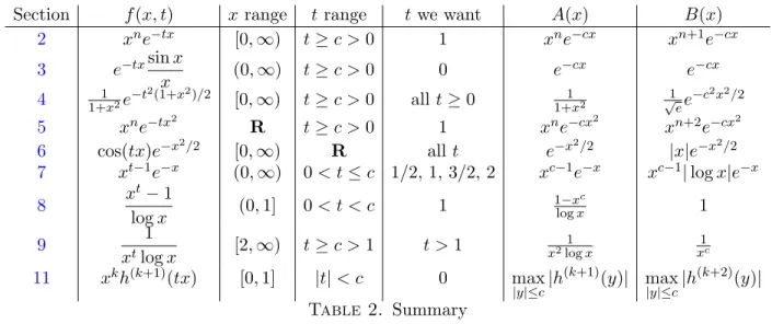
In Table 2 we include choices for A(x) and B(x) for the functions we have treated. Since the calculation of a derivative at a point only depends on an interval around the point, we have replaced a t-range such ast >0 with t≥c >0 in some cases to obtain choices for A(x) andB(x).

Section f(x, t) x range t range twe want A(x) B(x)

2 xⁿe^−tx [0,∞) t≥c >0 1 xⁿe^−cx xⁿ⁺¹e^−cx

3 e^−txsinx

x (0,∞) t≥c >0 0 e^−cx e^−cx

4 _1+x¹ 2e^{−t2(1+x2)/2} [0,∞) t≥c >0 all t≥0 _1+x¹2 √1

ee^−c2x2/2

5 xⁿe^−tx2 R t≥c >0 1 xⁿe^−cx2 xⁿ⁺²e^−cx2

6 cos(tx)e^−x2/2 [0,∞) R all t e^−x2/2 |x|e^−x2/2

7 x^t−1e^−x (0,∞) 0< t≤c 1/2, 1, 3/2, 2 x^c−1e^−x x^c−1|logx|e^−x

8 x^t−1

logx (0,1] 0< t < c 1 ^1−x_logx^c 1

9 1

x^tlogx [2,∞) t≥c >1 t >1 _x2log¹ x

1 x^c

11 x^kh^(k+1)(tx) [0,1] |t|< c 0 max

|y|≤c|h^(k+1)(y)| max

|y|≤c|h^(k+2)(y)|

Table 2. Summary

We did not put the function from Section10in the table since it would make the width too long and it depends on two parameters. Putting the parameter into the coefficient of cos²xin Section10,

we can takef(x, t) = 1/(t²cos²x+b²sin²x)ⁿforx∈[0, π/2], 0< c≤t≤c⁰(that is, keeptbounded away from 0 and∞), A(x) = 1/(c²cos²x+b²sin²x)ⁿ and B(x) = 2c⁰n/(c²cos²x+b²sin²x)ⁿ⁺¹. Corollary 12.4. If a(t) and b(t) are both differentiable on an open interval(c₁, c₂), then

d dt

Z b(t) a(t)

f(x, t) dx= Z b(t)

a(t)

∂

∂tf(x, t) dx+f(b(t), t)b⁰(t)−f(a(t), t)a⁰(t) for (x, t)∈[α, β]×(c1, c2), where α < β and the following conditions are satisfied:

• f(x, t) and _∂t^∂f(x, t) are continuous on[α, β]×(c₁, c₂),

• for all t∈(c1, c2), a(t)∈[α, β]and b(t)∈[α, β],

• for (x, t)∈ [α, β]×(c1, c2), there are upper bounds |f(x, t)| ≤ A(x) and |_∂t^∂f(x, t)| ≤ B(x) such that Rβ

α A(x) dx andRβ

α B(x) dx exist.

Proof. This is a consequence of Theorem12.3 and the chain rule for multivariable functions. Set a function of three variables

I(t, a, b) = Z b

a

f(x, t) dx

for (t, a, b)∈(c1, c2)×[α, β]×[α, β]. (Hereaand b are not functions oft, but variables.) Then

(12.3) ∂I

∂t(t, a, b) = Z b

a

∂

∂tf(x, t) dx, ∂I

∂a(t, a, b) =−f(a, t), ∂I

∂b(t, a, b) =f(b, t),

where the first formula follows from Theorem 12.3 (its hypotheses are satisfied for each a and b in [α, β]) and the second and third formulas are the Fundamental Theorem of Calculus. For differentiable functions a(t) andb(t) with values in [α, β] forc1 < t < c2, by the chain rule

d dt

Z b(t) a(t)

f(x, t) dx = d

dtI(t, a(t), b(t))

= ∂I

∂t(t, a(t), b(t))dt dt+ ∂I

∂a(t, a(t), b(t))da dt + ∂I

∂b(t, a(t), b(t))db dt

=

Z b(t) a(t)

∂f

∂t(x, t) dx−f(a(t), t)a⁰(t) +f(b(t), t)b⁰(t) by (12.3).

A version of differentiation under the integral sign forta complex variable is in [11, pp. 392–393].

Example 12.5. For a parametric integral Rt

af(x, t) dx, where a is fixed, Corollary 12.4 tells us that

(12.4) d

dt Z t

a

f(x, t) dx= Z t

a

∂

∂tf(x, t) dx+f(t, t)

for (x, t)∈[α, β]×(c1, c2) provided that (i)f and∂f /∂tare continuous for (x, t)∈[α, β]×(c1, c2), (ii)α≤a≤βand (c₁, c₂)⊂[α, β], and (iii) there are bounds|f(x, t)| ≤A(x) and|_∂t^∂f(x, t)| ≤B(x) for (x, t)∈[α, β]×(c1, c2) such that the integrals R_β

α A(x) dx and R_β

α B(x) dx both exist.

We want to apply this to the integral F(t) =

Z t 0

log(1 +tx) 1 +x² dx

fort≥0. ObviouslyF(0) = 0. Heref(x, t) = log(1 +tx)/(1 +x²) and _∂t^∂f(x, t) =_(1+tx)(1+x^x 2). To includet= 0 in the setting of Corollary12.4, the opent-interval should include 0. Therefore we’re going to considerF(t) for small negative ttoo.

Use (x, t) ∈[−δ,1/(2ε)]×(−ε,1/(2δ)) for small ε and δ (between 0 and 1/2). In the notation of Corollary 12.4, α = −δ, β = 1/(2ε), c1 = −ε, and c2 = 1/(2δ). To have (c1, c2) ⊂ [α, β] is equivalent to requiring ε < δ (e.g., ε = δ/2). We chose the bounds on x and t to keep 1 +xt away from 0: −1/2 < xt < 1/(4εδ), so 1/2 < 1 +xt < 1 + 1/(4εδ).³ That makes |log(1 +xt)|

bounded above and 1 +txbounded below, so|f|and|∂f /∂t|are both bounded above by constants (depending on ε and δ), so (12.4) is justified with A(x) and B(x) being constant functions for x∈[α, β]. Thus when 0< ε < δ <1 and−ε < t <1/(2δ),

F⁰(t) = Z t

0

x

(1 +tx)(1 +x²)dx+log(1 +t²) 1 +t²

= Z t

0

1 1 +t²

−t

1 +tx + t

1 +x² + x 1 +x²

dx+ log(1 +t²) 1 +t² . After antidifferentiating the three terms in the integral with respect to x,

F⁰(t) =

−1

1 +t² log(1 +tx) + t

1 +t²arctan(x) +log(1 +x²) 2(1 +t²)

t 0

+log(1 +t²) 1 +t²

= −log(1 +t²)

1 +t² +tarctan(t)

1 +t² +log(1 +t²)

2(1 +t²) +log(1 +t²) 1 +t²

= tarctan(t)

1 +t² +log(1 +t²) 2(1 +t²) . (12.5)

Letting δ →0⁺ shows (12.5) holds for allt≥0. SinceF(0) = 0, by the Fundamental Theorem of Calculus

F(t) = Z t

0

F⁰(y) dy= Z t

0

yarctan(y)

1 +y² +log(1 +y²) 2(1 +y²)

dy.

Using integration by parts on the first integrand withu= arctan(y) and dv= _1+y^y2 dy, F(t) =uv

t 0

− Z t

0

vdu+ Z t

0

log(1 +y²) 2(1 +y²) dy

= arctan(y)log(1 +y²) 2

t 0

− Z t

0

log(1 +y²) 2(1 +y²) dy+

Z t 0

log(1 +y²) 2(1 +y²) dy

= 1

2arctan(t) log(1 +t²), so

(12.6)

Z t 0

log(1 +tx)

1 +x² dx= 1

2arctan(t) log(1 +t²).

fort≥0. Both sides are odd functions of t, so (12.6) holds for allt. Settingt= 1, Z 1

0

log(1 +x)

1 +x² dx= 1

2arctan(1) log 2 = πlog 2 8 .

3Since−δ≤x≤1/(2ε) and−ε < t <1/(2δ),xt <max(εδ,1/(4εδ)), and the maximum is 1/(4εδ) whenε, δ <1/2.

13. The Fundamental Theorem of Algebra

By differentiating under the integral sign we will deduce the fundamental theorem of algebra: a nonconstant polynomialp(z) with coefficients inChas a root inC. The proof is due to Schep [13].

Arguing by contradiction, assume p(z) 6= 0 for all z ∈ C. For r ≥ 0, consider the following integral around a circle of radiusr centered at the origin:

I(r) = Z 2π

0

dθ p(re^iθ).

This integral makes sense since the denominator is never 0, so 1/p(z) is continuous on C. Let f(θ, r) = 1/p(re^iθ), so I(r) =R_2π

0 f(θ, r) dθ.

We will prove three properties of I(r):

(1) Theorem 12.3can be applied to I(r) for r >0, (2) I(r)→0 as r→ ∞,

(3) I(r)→I(0) as r→0⁺ (continuity at r= 0).

Taking these for granted, let’s see how a contradiction occurs. Forr >0, I⁰(r) =

Z 2π 0

∂

∂rf(θ, r) dθ= Z 2π

0

−p⁰(re^iθ)e^iθ p(re^iθ)² dθ.

Since

∂

∂θf(θ, r) = −p⁰(re^iθ)

p(re^iθ)² ire^iθ =ir ∂

∂rf(θ, r), forr >0 we have

I⁰(r) = Z 2π

0

∂

∂rf(θ, r) dθ= Z 2π

0

1 ir

∂

∂θf(θ, r) dθ= 1

irf(θ, r)

θ=2π θ=0

= 1 ir

1

p(r)− 1 p(r)

= 0.

ThusI(r) isconstantforr >0. SinceI(r)→0 as r→ ∞, the constant is zero: I(r) = 0 for r >0.

Since I(r)→I(0) asr →0⁺ we getI(0) = 0, which is false sinceI(0) = 2π/p(0)6= 0.

It remains to prove the three properties of I(r).

(1) Theorem12.3 can be applied to I(r) for r >0:

Since p(z) and p⁰(z) are both continuous on C, the functions f(θ, r) and (∂/∂r)f(θ, r) are continuous forθ∈[0,2π] and all r≥0. This confirms the first condition in Theorem 12.3.

For each r₀ >0 the set {(θ, r) :θ ∈[0,2π], r ∈[0,2r₀] is closed and bounded, so the functions f(θ, r) and (∂/∂r)f(θ, r) are both bounded above by a constant (independent of r and θ) on this set. The range of integration [0,2π] is finite, so the second condition in Theorem 12.3 is satisfied using constants forA(θ) and B(θ).

(2) I(r)→0 as r→ ∞: Let p(z) have leading term cz^d, with d = degp(z) ≥ 1. As r → ∞,

|p(re^iθ)|/|re^iθ|^d→ |c|>0, so for all larger we have |p(re^iθ)| ≥ |c|r^d/2. For such larger,

|I(r)| ≤ Z 2π

0

dθ

|p(re^iθ)| ≤ Z 2π

0

dθ

|c|r^d/2 = 4π

|c|r^d, and the upper bound tends to 0 as r→ ∞ sinced >0, so I(r)→0 as r→ ∞.

(3)I(r)→I(0) as r→0⁺: Forr >0, (13.1) I(r)−I(0) =

Z 2π 0

1

p(re^iθ) − 1 p(0)

dθ=⇒ |I(r)−I(0)| ≤ Z 2π

0

1

p(re^iθ) − 1 p(0)

dθ.

Since 1/p(z) is continuous at 0, for ε >0 there isδ >0 such that|z|< δ⇒ |1/p(z)−1/p(0)|< ε.

Therefore if 0< r < δ, (13.1) implies |I(r)−I(0)| ≤R2π

0 εdθ= 2πε.

14. An example needing a change of variables

Our next example is taken from [1, pp. 78,84]. For all t ∈ R, we will show by differentiation under the integral sign that

(14.1)

Z

R

cos(tx)

1 +x² dx=πe^−|t|. For example, takingt= 1,

Z

R

cosx

1 +x² dx= π e.

In (14.1), setf(x, t) = cos(tx)/(1 +x²). Sincef(x, t) is continuous and|f(x, t)| ≤1/(1 +x²), the integral in (14.1) exists for allt. A graph ofπe^−|t|is in Figure1. Noteπe^−|t|isnotdifferentiable at 0, so we shouldn’t expect to be able to prove (14.1) att= 0 using differentiation under the integral sign.

Figure 1. Graph of y=πe^−|t|. The caset= 0 of (14.1) can be treated with elementary calculus:

Z

R

dx

1 +x² = arctanx

∞

−∞

=π.

Since the integral in (14.1) is an even function oft, to compute the integral for t6= 0 it suffices to treat the case t >0.⁴

Let

F(t) = Z

R

cos(tx) 1 +x² dx.

If we try to compute F⁰(t) for t >0 using differentiation under the integral sign, we get

(14.2) F⁰(t)=^?

Z

R

∂

∂t

cos(tx) 1 +x²

dx=− Z

R

xsin(tx) 1 +x² dx.

Unfortunately, there is no upper bound |_∂t^∂f(x, t)| ≤B(x) that justifies differentiating F(t) under the integral sign (or even justifies that F(t) is differentiable). Indeed, when x is near a large odd multiple of (π/2)/t, the integrand in (14.2) has values that are approximatelyx/(1 +x²) ≈ 1/x, which is not integrable for large x. That does not mean (14.2) is actually false, although if we weren’t already told the answer on the right side of (14.1) then we might be suspicious about

4A reader who knows complex analysis can derive (14.1) fort >0 by the residue theorem, viewing cos(tx) as the real part ofe^itx.