Autonomous onboard guidance and navigation performance for Earth to Mars transfer missions

Autonomous Onboard Guidance and Navigation Performance

for Earth to Mars Transfer Missions

by

Peter J. Neirinckx

S.B., Massachusetts Institute of Technology (1990) Submitted to the Department of Aeronautics and Astronautics

in partial fulfillment of the requirements for the degree of Master of Science in Aeronautics and Astronautics

at the

MASSACHUSETTS INSTITUTE OF TECHNOLOGY

January 1992

@

Author ... ... 4.... ... ....

Department of Aeronautics and Astronautics January 16, 1992

Certified by ...:. ...,..-... ..

Professor Richard H. Battin Adjunct Professor. of Aeronautics and Astronautics Thesis Supervisor Certified by...

Certified by... Principal Member,

Kenneth M. Spratlin Group Leader, The Charles Stark Draper Laboratory, Inc.

Technical Supervisor ....

... Y z..- Iey... ... .

Sfanley W. Shepperd

Technical Staff, The Charles Stark Draper Laboratory, Inc. Technical Supervisor

Accepted by ... ... ... ... ... ...

SProfessor Harold Y. Wachman MAs4 ':Fs _{~u'ma Chairman, Departmental Graduate Committee}

,F

~

0 1992

I ýý r .

-• '-•-''-•- .•..

Autonomous Onboard Guidance and Navigation Performance

for Earth to Mars Transfer Missions

by

Peter J. Neirinckx

Submitted to the Department of Aeronautics and Astronautics on January 16, 1992, in partial fulfillment of the requirements

for the degree of

Master of Science in Aeronautics and Astronautics

Abstract

In preparation for manned missions to Mars, autonomous onboard guidance and nav-igation is studied as a backup to ground-based navnav-igation systems. A survey of the literature indicates that autonomous interplanetary navigation is viable and desirable. However, due to the reliability and accuracy of ground-based methods, little has been done in this area. for the past two decades. Since that time, the accuracy and reliability of onboard navigation instruments have improved significantly. A refinement of the older studies is performed by developing an interplanetary autonomous navigation and guid-ance (AG&N) computer simulation. A linear error covariguid-ance analysis provides the basis for the simulation, and an Earth to Mars Hohmann transfer mission defines the base-line interplanetary trajectory. The development is extensively detailed, and citations are

provided to promote future reference.

The interplanetary simulation is coupled to an existing Mars approach computer simula-tion [Shepperd, S. W., et al, Onboard Preaerocapture Navigasimula-tion Performance at lMars, AAS Paper 91-119, 1991]. Both the interplanetary and approach performances for a sample Mars a.eroca.pture mission are examined based on several convenient figures-of-merit. It is found that the mission can be performed successfully using only AG&N during the entire mission. A parameter sensitivity analysis is also performed, resulting in a more comprehensive understanding of the AG&N problem. Further investigations are suggested.

Thesis Supervisor: Professor Richard H. Battin

Title: Adjunct Professor of Aeronautics and Astronautics Technical Supervisor: Kenneth M. Spratlin

Title: Group Leader, The Charles Stark Draper Laboratory, Inc. Technical Supervisor: Stanley W. Shepperd

Acknowledgments

I am truly grateful to CSDL for the opportunity to have pursued my studies at MIT

and to have gained so much experience in the astrodynamics field. I would like to thank Professor Dick Battin for his inspirational teaching. Space exploration continues in the world today in part because of the excitement Professor Battin fosters. I would like to recognize and thank Stan Shepperd for his support, patience, and insightful guidance throughout the past months. Ken Spratlin and Tim Brand deserve many thanks for their helpful directions and the original thesis concept. Much appreciation is also conveyed to Wayne McClain for his initial help at CSDL and for his encouragement of further pursuits.

To my mother and father, I would like to especially express my gratitude. Their con-tinued love and devotion I deeply cherish. They, along with Sandra, John, and Cheryl, are my foundation. To all the friends along the way who have shared of themselves and have lent an ear: thank you Anthony, Catherine, Cindy, Dennis, Kate, Steve, Susan and many more!

I would like to dedicate this thesis to my grandfathers, Wilmer Kenney and Edward

This report was prepared at The Charles Stark Draper Laboratory, Inc. under NASA Contract NAS9-18426. Publication of this report does not constitute approval by the Draper Laboratory or the sponsoring agency of the findings or conclusions contained herein. It is published for the exchange and stimulation of ideas.

I hereby assign my copyright of this thesis to The Charles Stark Draper Laboratory, Inc., Cambridge, Massachusetts.

Peter Joseph Neirinckx Permission is hereby granted by The Charles Stark Draper Laboratory, Inc., to the Massachusetts Institute of Technology to reproduce any or all of this thesis.

List of Acronyms and Symbols

Note: A bold-face, lower-case symbol indicates a vector quantity while a bold-face, upper-case symbol indicates a matrix quantity. The magnitude or trace of the symbol is indi-cated by normal-face text.

Symbol Description

AG&N autonomous (interplanetary) guidance and navigation

DSN Deep Space Network

ECRV exponentially correlated random variable

EI entry interface (atmosphere at 125 kilometers above Martian surface)

FOM figure-of-merit

FOV field-of-view

fps feet per second

GPS Global Positioning System

hrs hours

IMU inertial measurement unit

KF Kalman filter

LOS line-of-sight (generally to Mars), LOS coordinate system (with x = LOS direction and z = angular momentum direction of the s/c trajectory) LVLH local vertical / local horizontal coordinate system (with y = radial

direction and z = trajectory angular momentum direction)

m/s meters per second

OD orbit determination

PN process noise

rms root mean square

ls•c arcseconds

s/c spacecraft

SOI sphere of influence at Mars TCM Trajectory Correction Maneuver

wrt with respect to

a semi-major axis (of trajectory or error ellipsoid)

b semi-minor axis (of error ellipsoid); bias percentage

B linear guidance matrix

e state uncertainty vector, eccentricity vector

E state covariance matrix

DD velocity correction uncertainty matrix DV velocity correction matrix

Av state uncertainty vector

h periapse altitude; angular momentum magnitude

i I k A M N

Q

t

Ex

X

identity matrix of appropriate dimension Kalman gain vector

aerocapture FOM compatibility matrix

integrated process noise matrix

gravitational constant (solar or Martian); micro angle between error ellipsoid semi-major axis and (linear) state transition matrix

process noise matrix inertial position vector

standard deviation (or 3o), equal to (three times) quantities with zero mean values

time unit vector

inertial velocity vector state vector

actual state error vector estimated state error vector

6 x 6 mean squared actual error matrix, position and velocity

6 x 6 position and velocity error correlation matrix (actual to estimated)

Subscripts act E

f

II

final (nominal SOI or periapse) angular momentum

hyperbolic measured nominal periapse

Mars rotational axis reference value, nominal Mars relative

Description

degrees

value immediately after a measurement or TCM first total time derivative

second total time derivative third total time derivative transpose

defined x axis

List of Figures

2-1 The State Uncertainty Vector ... .. . .. ... . 11

2-2 Relative Geometry for the Optical Measurement ... 27

2-3 Example Star Tracker Pixel Array ... ... 28

2-4 Geometry of the Same-Plane Centroid Bias ... 29

3-1 Minimizing the Cost of VTOA Guidance ... 44

3-2 The Compensation Vector for VTOA Guidance ... 45

3-3 Plot of Equation 3.37 ... 47

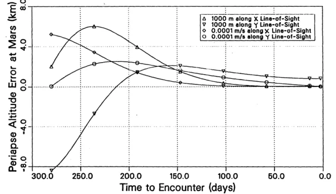
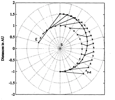
3-4 Periapse Altitude Sensitivity to State Errors in a Mars LOS Coordinates 47 4-1 The Baseline Hohmann Trajectory ... 58

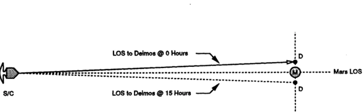
4-2 Geometry of the Deimos sightings ... ... .. 60

4-3 Linear Approximation to Obtain the Process Noise Velocity Components 63 4-4 Simulation Flowchart ... 66

4-5 Aerocapture Accuracy Requirements (1) at Entry Interface ... 67

4-6 Aerocapture Accuracy Requirements (2) at Entry Interface ... 68

4-7 Cartoon of a 1 SOL Orbit ... 68

4-8 Current Position Uncertainties in Mars LOS Coordinates ... . . 70

4-9 Current Position Uncertainties in LVLH Coordinates. ... . 70

4-10 LOS and LVLII Coordinate Definitions ... 71

4-11 Position Uncertainties in LVLH Coordinates: No Navigation ... 71

4-12 Planetary Distances and LOS Rates for the Hohmann Transfer. ... . 73

4-13 Final Approach for the Hohmann Transfer ... . . . 73

4-14 Optical Angular Diameters of the Planets ... 7.5 4-15 Optical Angular Diameters of the Mars System ... . . 75

4-16 SOI Position Uncertainties in Mars LOS coordinates ... . . 76

4-18 Position Error Ellipsoids at the SOI, at EI, and at Periapse ... .. 77

4-19 Effect of Dynamics on Errors With No Navigation During Mars Approach 77 4-20 Periapse Altitude and Inclination Uncertainties ... .78

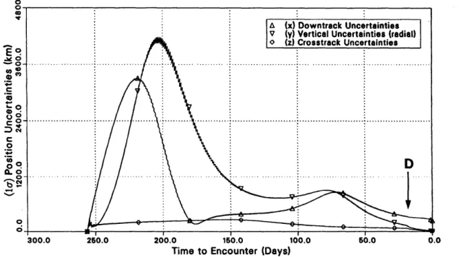
4-21 SOI Position Uncertainties in Mars LOS coordinates: Baseline simulation without course corrections ... 79

4-22 Current RMS Velocity Uncertainties in Mars LVLH Coordinates ... . 79

4-23 SOI Velocity Uncertainties in Mars LVLH Coordinates ... 81

4-24 Periapse Altitude and Inclination Dispersions Showing FTOA Targeting Accuracy ... ... ... 81

4-25 FTOA Cost to Correct for LOS Errors ... 82

4-26 Baseline Performance for Three Cases of the Approach Simulation . . . . 84

4-27 Baseline Performance for The Optical Case of the Approach Simulation . 85 4-28 Relative Geometry of the Error Ellipsoid for Approach Navigation . . . . 85

5-1 Approach Navigation Figures-of-Merit for Variational Case 2 ... 93

5-2 LOS Position Uncertainties for Variational Case 3 ... 94

5-3 LVLH Velocity Uncertainties for Variational Case 3 ... 94

5-4 Approach Navigation Figures-of-Merit for Variational Case 7 ... 96

5-5 Mars Observer Trajectory: x-y planar projections ... 100

5-6 Sprint Trajectory: x-y Planar Projections ... 101

5-7 Approach Navigation Figures-of-Merit for Variational Case 12 ... 101

5-8 Earth-LOS Current Position Uncertainties: Doppler tracking of Earth without optical measurements ... .. 103

5-9 Earth-LOS Current Position Uncertainties: Range tracking of Earth with-out optical measurements ... 104

5-10 Approach Navigation Figures-of-Merit for Variational Case 16 ... 106

6-1 Monte Carlo Simulations Varying a Four TCM Schedule ... 112

D-1 Coordinate System for Minimizing the Velocity Correction ... 127

D-2 Solution for the Optimal Velocity Correction ... 128

E-1 LOS Position Uncertainties for a Case with No Earth Measurements . .. 134

List of Tables

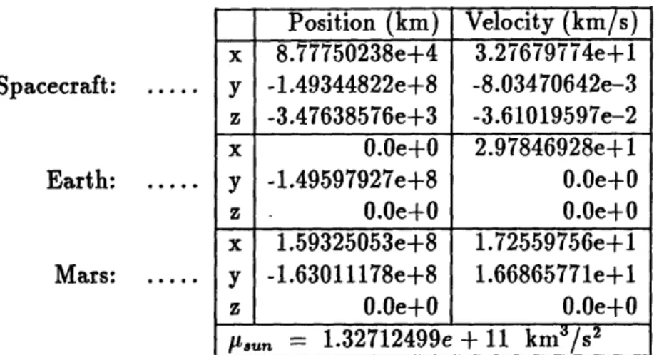
4.1 Two-Body Initial Conditions For The Baseline Mission ... 59

4.2 A Priori Error Covariance (Eo) Diagonals ... 62

4.3 The Effects of Time Step on the Process Noise Integral (N) Approximation 64 4.4 Components of the Baseline Scenario ... 65

4.5 Course Corrections for the Baseline Run ... 80 4.6 Inertial Error Covariance and State for Mars Approach Hand-Over .... 83

5.1 Performance for Variations About the Baseline Scenario at the SOI, EI,

and Periapse (Part 1) ... 88 5.2 Performance for Variations About the Baseline Scenario at the SOI, EI,

and Periapse (Part 2) ... ... 89 5.3 Description of Objectives for the Variational Cases ... 90

5.4 Approach Navigation Performance for Four Variational Cases ... 91 5.5 Initial Conditions for the Mars Observer Variation: Inertial Coordinates. 99 5.6 Initial Conditions for the Sprint Orbit Variation: Inertial Coordinates... 100 E.1 List of Variations About Case 9 ... ... 133

Contents

1 Introduction

1.1 Background and Motivation . . . . . 1.2 Performance Analysis Objectives . . 1.3 Method and Assumptions . . . .

1.4 Thesis Overview... 2 Navigation Theory

2.1 Choice of State Variables . . . . 2.2 Linear Filter Development . . . .

2.2.1 Consider States . . . ...

2.3 State Propagation... 2.3.1 Position and Velocity States .

2.3.2 Bias States ...

2.3.3 Propagation of the Covariance 2.3.4 Process Noise ...

2.3.5 Performance Parameters . . . 2.4 Observation Models...

2.4.1 Optical Measurements . . . . 2.4.2 Radiometric Measurements. . 2.4.3 Optimum Measurement Selecti,

2.5 Navigation Instrument Errors . .

. . . . . . . . . . . . . . ... ... . . . . . . . . ... Matrix. . . . ... . . . . . . . . Matrix ...

. . . .

. . . .

3.2 Fixed Time-of-Arrival Guidance ... 3.2.1 The Dispersion Matrix ...

35 36 36 39

3.2.2 Potential Guidance Accuracy . . . 3.3 Variable Time-of-Arrival Guidance . . . . 3.4 Periapse Altitude and Inclination Guidance

3.4.1 Periapse Only ...

3.4.2 Periapse and Inclination . . . . 3.5 Burn Execution Errors . . . . 3.5.1 Known and Unknown Errors . . . . 3.5.2 Three Models ...

3.6 Course Correction Scheduling . . . . 4 Typical System Performance

4.1 Baseline Mission ...

4.1.1 The Nominal Trajectory ... 4.1.2 Navigational Design ... 4.1.3 Guidance Design ... 4.1.4 Summary ...

4.2 Navigation Performance Requirements . . . . 4.3 Simulation Results & Analysis . . . . 4.3.1 Interplanetary Navigation . . . . 4.3.2 Mars Approach Navigation . . . . 4.3.3 Summ ary ...

5 Variational System Performance and Sensitivity 5.1 Navigational Sensitivities to Error Sources . . . .

5.1.1 Mechanical Error Sources . . . .

5.1.2 Environmental and Filter Error Sources ..

5.2 Sensitivities to the Environment . . . . 5.2.1 Modified Measurement Schedule . . . . 5.2.2 Alternate Mission Trajectory . . . . 5.2.3 Inclusion of Radiometric Data . . . .

5.2.4 Backup System Role ...

5.3 Guidance Sensitivities . . . .

5.3.1 Mechanical Error Sources . . . .

5.3.2 Alternate Guidance Scheme . . . .

Analysis . . . 0 0 . . . 0. ° , ... o 87 92 92 95 95 95 98 102 102 104 105 105

5.3.3 Modified Correction Schedule ... 107

6 Conclusions 109

6.1 General Summary ... ... 109

6.2 Summary of Sensitivity Results . . . . 110

6.3 Future Research ... 111

Bibliography 113

A Extensions to Process Noise Derivation 117

B Alternate Guidance Methods 120

C Time of Periapse Passage Sensitivity 124

D Nominal Orbit Construction 125

Chapter 1

Introduction

The United States has recently expressed a renewed interest in sending a human crew to the planet Mars. As with the Apollo moon missions, the concern for crew autonomy has surfaced. Especially in the event of problems, it may be desirable for the spacecraft (s/c) to have the ability to perform navigation or trajectory maneuvers not under ground-based mission control. An onboard interplanetary autonomous guidance and navigation (AG&N) system is required to accomplish this goal. An autonomous system is one in which all navigational measurements and calculations are performed using instruments onboard the s/c; guidance is by definition an onboard problem'. Because of power limitations, only optical measurements of stars and other heavenly bodies generally fit the autonomous description. Other data types such as 1-way radiometric measurements can also be considered as supplemental, though not truly autonomous. This thesis presents a detailed AG&N system description and performance analysis in order to determine the feasibility of such a system when applied to a Mars mission.

1.1

Background and Motivation

The concept of interplanetary AG&N is not new. Numerous studies have been conducted beginning in the early 1960's to explore AG&N capabilities [2], [6], [17], [26], [40]. Indeed, the concept has been demonstrated to some extent by the Mariner '71 mission [10]. Recent surveys of earth-orbiting AG&N capabilities were made in 1983 [12], 1984 [5],

1

A guidance capability acts through the propulsion system which is a physical component of the spacecraft.

and 1985 [27]. This thesis brings together many of the techniques and results from those reports. Several sources will be cited often and are considered complementary reading. The studies are by Cicolani et al. [6], [40], and Shepperd, et al. [33]. Battin's textbook [3] is also a useful source.

The number of interplanetary AG&N studies, however, began to decline in the early seventies2. The Deep Space Network (DSN) began to provide ground-based tracking for the infrequent unmanned interplanetary missions. The DSN worked (and still performs) very well, providing excellent coverage, reliability, and most importantly, accuracy. As a result, few studies have applied current autonomous instrument accuracies to the inter-planetary navigation problem. This thesis intends to show that with these new instru-ments, autonomous navigation provides adequate performance support for interplanetary navigation and guidance. In particular, the interplanetary mission studied in this the-sis is one in which the capture into Mars orbit is accomplished through an aerocapture maneuver instead of propulsive capture. Since aerocapture imposes tighter guidance and navigation accuracy requirements, less restrictive missions are assumed to be adequately supported if a similar aerocapture mission can be supported.

Guidance mechanisms and accuracies have also improved over the past twenty years. The coupling between interplanetary guidance and navigation performance becomes an important issue when considering that the interplanetary spacecraft may be large, re-quiring long burns with active control. This thesis addresses this issue by means of a dispersion analysis.

The primary motives for studying the interplanetary AG&N problem are to update the general knowledge of AG&N capabilities and to consider the possibility of a backup system to the DSN. Other motivations exist and are briefly described below.

Motivation Summary and Problem Statement

This thesis is motivated by the presence of the following possibilities:

* Especially for a manned mission, a backup AG&N system is always desirable. Au-tonomous navigation could be used to supplement the DSN, act as a system backup, or replace it entirely in certain cases.

2_{Distinguished from Earth-bound AG&N where numerous studies have been performed, especially in} the 1980's with the advent of the Global Positioning System.

* Previous studies have made certain approximations due to computational

consid-erations. In order to keep the problem simple, some AG&N covariance studies did not include process noise or estimated only a small number of states. Current computational facilities can support more complex analysis.

* On-board navigation instrumentation accuracies have improved since the last stud-ies. Also, the interplanetary mission objectives and requirements have changed significantly (i. e. can an AG&N system provide accuracies sufficient to support aerocapture?). The former studies do not indicate a capability to handle the new requirements. Verification of mission support with current capabilities is needed. * The DSN is expensive to operate [12]. If a reliable cost-effective alternative system

with comparable performance exists, it should be investigated.

* The ability of a s/c to maneuver autonomously in interplanetary space could also facilitate new applications. Specifically, future missions may involve multiple s/c in flight at one time which ground-based systems may not be able to efficiently support. Furthermore, small (robotic) spacecraft that could fly safely under their own control, temporarily or continuously, would be a step toward the increased exploration of the solar system.

1.2

Performance Analysis Objectives

Given the above motivation for autonomous navigation of interplanetary spacecraft, the focus logically switches to answering the following question:

Problem Statement: "Can present-day autonomous guidance and navigation

instru-mentation provide sufficient interplanetary trajectory accuracy for a successful aerocap-ture mission?"

A study by Shepperd, et al.[33] has previously analyzed the autonomous Mars ap-proach (approximately two days prior to Mars atmosphere entry interface) navigation problem, with interplanetary navigation provided by the DSN. This thesis essentially extends the autonomous approach performance analysis to the interplanetary Earth to Mars trajectory in an attempt to answer the Problem Statement and demonstrate the current capabilities of AG&N for general interplanetary missions.

Also, by interpreting the Problem Statement as a feasibility philosophy, a baseline mission should be chosen such that if the requirements are not met for that mission, it can then be assumed that the requirements cannot be met for other missions. A secondary objective of the study is to provide some insight into the system performance through trajectory dynamics, geometry variations, and guidance/navigation interaction.

1.3

Method and Assumptions

An AG&N simulator has been developed in the HAL/S programming language on an IBM 3090 mainframe computer at The Charles Stark Draper Laboratory, Inc. The simu-lation and baseline mission constitutes various assumptions about the guidance hardware, navigation instrumentation, and their inherent accuracies. The baseline autonomous nav-igation is accomplished only through optical measurements. The computer simulation performs a linear covariance analysis on the associated guidance and navigation errors. As such, the analysis is only valid when the linearity assumptions are justified. The output of such a simulation is a statistical representation of the performance that can be expected from any mission similar to the nominal baseline mission.

For a successful mission, it is generally desired that the spacecraft position and veloc-ity errors be kept small in order to keep the fuel and structure costs down. The abilveloc-ity to maintain or sustain small errors is the purpose of navigation and the goal of guidance. The definition of "small" is somewhat ambiguous, but generally means that if the Tay-lor series of a function is taken, the quadratic and higher order terms can be neglected since they are much "smaller" than the linear term. This "linearization" assumption is paramount in this thesis. Linearization makes the effects of deviating from the nominal3 trajectory transparent. In other words, "error" terms evaluated off the nominal, but at the same time, tend to have similarly valued derivatives. This effect is useful when trying to get a qualitative feel for the effectiveness of AG&N for different missions.

To make a linear assumption, some knowledge of both the error type and the error's functional relationships with desired quantities are needed. The particular types of errors from navigational inaccuracies, guidance inaccuracies, and elsewhere are diverse but do share an important characteristic. These error sources are generally stochastic in na-ture and can be modeled as having Gaussian distributed values with zero means. Since

the desired quantities such as terminal miss uncertainty have been linearized about the nominal, they are linear combinations of the state error variables. The desired quantities are then Gaussian as well, and the AG&N analysis need only consider the covariances of the quantities of interest to get a complete statistical description of the desired parame-ters. A covariance analysis is then the appropriate methodological tool for this study. In particular, the standard Kalman Filter (KF) has been chosen to optimally incorporate the navigational measurements. The guidance equations are also incorporated into this formulation. Though a deterministic Monte Carlo study can obtain similar results, that method is very inefficient because of the large number of computer simulations required. In contrast, the structure for this study is a linear error covariance analysis which requires only a single run.

Below is a brief list of the assumptions made in this thesis. The list is intended to enable the reader to interpret the derivations and results in the following chapters appropriately and to formulate future work concisely.

Major Assumptions

* As with most other referenced studies, movement of the s/c with respect to (wrt) the Sun and planets will be governed by two-body (conic) dynamics. The planets' orbits are also conic. In addition, a patched-conic technique is used to propagate through the Mars sphere-of-influence (SOI), itself another mathematical approximation. * Any equations describing various error quantities will be linearized about the

nomi-nal mission trajectory by assuming the errors are small with respect to the nominomi-nal value but much larger than the second-order terms.

* Navigational measurements that require stellar direction vectors will use ficticious stars conveniently located. It is believed that the added complexity of adding a star catalog to the simulation is unnecessary. A sufficient number of adequate magnitude real stars can be found near a strategically placed ficticious star. Being near the ficticious star means that the first-order navigation sensitivity to star position should be the same. In other words, the information derived from either real or ficticious star is essentially identical.

* Trajectory Correction Maneuvers (TCM's) are applied impulsively. It is important to distinguish between correction maneuvers and rocket firings that exist as part of

the precomputed nominal path (e. g. plane change maneuvers or injection burns).

Some missions require some form of continuous thrusting or multiple impulsive

thrusts

_{as part of the nominal path so that the target can be reached in a time}

shorter than a free-fall path

_{. The nominal trajectories of this study avoid using}

any maneuvers as part of the reference trajectory.

* Error sources are modeled as either white noise or exponentially correlated random variables (ECRV). Their statistics will be given in later sections.

1.4

Thesis Overview

This thesis simulates an AG&N system to analyze its performance capabilities. Chap-ters 1, 2, and 3 draw from the various cited works to describe the nominal mission and develop the simulator. The detail of these chapters is such that the they are also intended to serve as a guide for future linear covariance studies. Chapter 4 applies the simulator to a baseline mission in order to show the feasibility of AG&N. Chapter 5 then performs a sensitivity analysis on the system in order to determine the critical assumptions made and their characteristic effect(s) on the AG&N system performance. Chapter 6 summa-rizes the major points of this thesis and provides suggestions for further study. Lastly, there are five appendices which elaborate on various topics from the main text.

4It is possible for a single injection burn to result in a sprint trajectory, but it would be very costly. SAn orbit that requires an impulsive injection burn.

Chapter 2

Navigation Theory

The purpose of navigation is to take measurements of the surrounding environment in order to improve the current knowledge of the vehicle state (position and velocity). Due to the presence of random errors in the measurements, only an approximate knowledge can be obtained. However, the use of an optimal filter to incorporate the measurement information minimizes the error in the knowledge of the state. This chapter discusses the particular quantities to be estimated, the choice of filter, processing of measurements, and the error sources modeled in the linear covariance simulator developed for this thesis.

2.1

Choice of State Variables

This section describes those key state parameters that are to be included in the estimation process. In theory, all the variables and parameters of the problem are random variables and should be estimated since, in fact, every "constant" physical quantity has been measured' and is subject to random measurement errors. Additionally, the errors in the random values are generally modeled as Gaussian with a zero mean value. Thus, all biases in the variables and parameters must also be estimated by the filter. In order to keep the problem tractable, only those quantities that are essential to the study of navigation performance are included in the generalized state vector, x.

An important aerocapture performance parameter, or figure-of-merit (FOM), is the periapse altitude, hp, of the s/c at the target planet (see [331). This and other performance parameters can be derived from knowledge of the s/c position and velocity vectors, r and

v, and the gravitational parameter pL of the sun or planet. Both r and v must be

estimated, but the gravitational parameter error is not estimated in this study. The position and velocity vectors of the planets in the sun-centered inertial system will also be considered known and not included in the estimated state. Any quantity that is not estimated in the simulation is considered to be known to a sufficient degree, or have such a small effect on the quantities of interest, that their value's uncertainty will not affect the navigation system performance results.

Errors produced by the navigation instruments are of interest because they often have a significant impact on the errors in the state estimate. The primary measurement type used for interplanetary navigation is the optical angle measurement between two heav-enly bodies (usually a star and a planet). The errors in measuring the angle (including finding the centroid of the planet) are estimated. Specifically, the errors in the angle measurements are modeled as an unknown random bias for each of the two components on the pixel array. The errors arise from several sources and will be discussed in Sec-tion 2.5. The errors are grouped together as a single white noise source and modeled as an exponentially correlated random variable (ECRV). The errors in determining the centroid are also modeled as ECRV's for each of the two components. Centroiding errors arise from the accuracy to which the shape of the lit limb of the planet can be defined.

Included in the state vector are components to estimate inaccuracies in radiometric measurements. These are not included for the baseline study (which relies on optical data only; see Chapter 4), but are used for several variational simulations in Chapter 5. Doppler and range data are 1-way2 as opposed to 2-way where Earth stations return signals to the s/c. The 1-way measurements are less accurate than the 2-way for two reasons. First, the clock hardware accuracy onboard the s/c generally has higher long and short period frequency drift rates than the Earth-based hardware. Second; with a 2-way measurement, any relative bias that exists between the Earth and s/c based clocks can be eliminated. Of course, the 2-way measurement cannot be included here as a truly autonomous measurement. With 1-way measurements, the estimated quantities are Doppler and range biases as well as s/c clock drift (which can be thought of as a range bias drift rate).

2

The 15 dimensional generalized state vector used in this thesis is defined as: r v 01 02 ecb1 ecb2 mcb1 mcb2 db rb rd

: inertial position vector : inertial velocity vector

: x-axis star tracker angle bias

: y-axis star tracker angle bias

: x-axis Earth centroid bias

S : y-axis Earth centroid bias

: x-axis Mars centroid bias

: y-axis Mars centroid bias

: Doppler velocity bias

: range distance bias

: range drift rate

2.2

Linear Filter Development

In a performance analysis, estimating the actual state is not a concern. Rather, quan-tifying the state error behavior in response to navigation (and guidance) system errors is of concern. In other words, the specific path is less important than the path of the errors. A Kalman Filter (KF) uses the statistics of the measurement errors as part of a weighted-least-squares state estimation process. Utilizing the covariance update portion of the KF provides the analysis a foundation from which to statistically describe the state errors without processing actual measurements or obtaining actual estimates of the state variables.

Of the various possible Kalman techniques of processing the measurements, a Sequen-tial KF is chosen3_{. The Extended KF, requiring an estimated state, is not chosen, nor is}

a higher order filter since the errors are expected to be small.

The construction of the Kalman Filter as applied to this analysis begins with the definition of the state error vector, e, as the difference between the estimated and ac-tual state vectors. The error vector contains the quantities to be minimized by the incorporation of measurements. Under the linear assumption of small deviations from a

SA Sequential KF is used for most preliminary performance studies because the measurements need

not be stored.

(precomputed) nominal trajectory, the equivalent expression is given in Equation 2.1.4

A graphical representation of this equation using only three states is given in Figure 2-1.

e

= ,X-

x

= (xno + bX) - (xnom±

+

) = bi - SX

(2.1)

The vector being estimated is actually 6x. For an unbiased estimator (filter), the mean

error in the estimate is zero. Thus, e post-multiplied by its transpose is exactly its covariance, E. This relationship is shown in Equations 2.2 and 2.3. Note that the E

matrix is symmetric.

= SiX-6x = 0 (2.2)

E - (e - )(e -

)T

= eeT

(2.3)

The Kalman Filter uses the E matrix, the sensitivity matrixs _{of the measurement}

(H) and the measurement error statistics matrix (R) to weight each measurement in such a way as to optimally estimate the state. The matrix form of the sensitivities and measurement statistics will be given in Sections 2.4 and 2.5, respectively. The measurements in this study are taken to occur at discrete moments in time instead of continuous measurements. Equations 2.4 and 2.5 are the standard discrete form of the Kalman covariance update (see Gelb [14], pg. 110). The matrix K is the Kalman gain matrix that adjusts the "weight" given the measurement. The matrix H is the measurement sensitivity matrix described in Section 2.4. The "+" denotes the matrix just after the measurement.

K = EHT[HEHT + R]-I (2.4)

E(+) = (I - KH)E (2.5)

The matrix I is the identity matrix commensurate in size with E. For a scalar measurement (such as the angle between lines-of-sight to a star and a planet) of variance

4In a purely navigational analysis, 6x is taken to be zero. However, guidance is also to be examined in Chapter 3 and requires six additional states in the state vector describing 6x, now non-zero.

Actual Trajectory

Nominal Trajectory

-nom

A

e =

e 8xe

Figure 2-1: The State Uncertainty Vector.

r2, the matrix HT reduces to the vector h and the gain matrix K reduces to the vector k.

The Kalman update of the covariance matrix in Equation 2.5 then reduces to the form in Equation 2.6. Note that the matrix inversion has been replaced by a simple division.

EhhTE

E(+) = E - hTE (2.6)

hTEh

+

02

2.2.1

Consider States

When the random character of a state variable is not well defined, yet removing the variable from the state vector is unwarranted, the variable can be redefined as a consider state. A consider state has the characteristic that its effect on the other states is "con-sidered" but the actual state itself is not estimated; a measurement does not change the variance of the consider state. This effectively means that the correlations with the con-sider state still change during the measurement update while the concon-sider state variance (diagonal term of E) does not change. Redefining a state variable to be a consider state is useful in determining the characteristic effect of that variable on the other states.

A modified version [34] of the "Joseph" form (Equation 2.7) of the Kalman update

permits the incorporation of consider states6 _{by allowing a generic (sub-optimal) gain}

vector k'. The form is also computationally efficient with no matrix multiplies. The new gain vector (for a 3 x 3 example) is given by Equation 2.8.

E(+) = (I - khT)E (I- khT)T + •~kkT (2.7)

k'

[

0

For this case, the updated covariance is

ell e12 e_{1 3} e12 e13 e2 2 e23 e23 0 (2.9)

(2.8)

The form for the update equation is now

E(+) = E- (wwT _ wIwT)

hTw +C2

0

(h

)(k

k)

w'= 0 = (hrEh+ •,2)(k- k')

W3

The inclusion of a consider

optimal gain. Another way of

By including the factor (1 + P)

measurements can be reduced.

state changes the gain from the optimal gain to a

sub-achieving a similar effect is through "underweighting."

in the calculation for the gain matrix, the sensitivity to

kunderweighting = (1

+)hEh

(2.11)

(1 +

+)hTEhT

Typical values for

/

Battin [3], pg. 677.

where

w= Eh,

Underweighting is more often used for sub-optimal "tuning" of onboard filters rather than in pre-mission covariance analysis.

2.3

State Propagation

Once E has been updated at a specific time by one or more discrete measurements, it must be propagated in time to the next measurement time. This is done by linearizing the equations of motion for the position and velocity errors about the nominal trajectory, and assuming a linear form for the other bias states. This section gives the propagation equations first for position and velocity errors, then for the bias states, and finally for the covariance matrix E itself.

2.3.1

Position and Velocity States

The two-body non-linear equations of motion (EOM) for position and velocity are

r = v v = -9r (2.12)

where ir, is the unit position vector. A simple Kepler routine is used to evaluate the EOM at any time given the initial conditions. Linearizing about the nominal state, x,,,,, the first order linear differential equation for propagating state errors is

6x = F(t)bx (2.13)

where

F =

G 0

(2.14)

and G is the gravity gradient matrix given by

G = 3u r (2.15)

Equations 2.13, 2.14, and 2.14 will be important when deriving the propagation equa-tion for E in Secequa-tions 2.3.3 and 2.3.4.

Large Time Step Formulation

The propagation of the state via direct integration becomes cumbersome if at each point along the trajectory, the effect of a measurement on some performance criteria at the end of the trajectory is checked. The number of calculations is then nearly squared7. An alternative method is via the state transition matrix, T(tl, to). The state transition method propagates the state error vector from time to to time tl in a single step. The matrix is found by linearizing the state at time tl about the reference state at to.

x (t,x(to)) = X(t1,x,,ef(to)) + (X(to)- xre(to)) + 02(6xo) (2.16)

xVo)=X(t₀o)IXretE) 6x

(tx1 t(2.17)

6X ~ x1 = (tl,to)6Xo (2.18)

The cartesian form for 41 is well known. Shepperd's [35] derivation is implemented in the simulator to propagate the state just after a measurement to the Mars encounter date. Two other possibilities exist for calculating the 4I matrix.

Element Formulation

For very large time steps, generally on the order of multiple orbits, an element formulation is often used. In this case, a different development for the measurement partials from the previous section is necessary. The advantage of using a two-body element formulation is that f is generally very simple; differing from the identity matrix by only one component. Using the equinoctal element set, let

'The total number of integration steps would become: N = n(n + 1)/2 where n is the previous

100000 010000 0 01000 0 _p element = 0 a = -1.5 At - (2.19) 0 0 0 1 00 a5 000010 a00001

where a is the semi-major axis. The above matrix reserves the first element for the semi-major axis and the sixth for the mean anomaly difference. After the simple prop-agation for small deviations in the elements, the results can then be transformed into cartesian coordinates. Shaver [32] gives the necessary transformation (Jacobian) matrix if equinoctal elements are used.

Small Time Step Formulation

Of course, 4 can be applied to small time steps as well as large time steps. The transition matrix is related to the dynamics matrix F by differentiating Equation 2.18, and using Equation 2.13 to get

I

= F

l(to,

to) = I

(2.20)

In theory, this may be integrated to get f(tx, to). However, for short time spans, F can be taken to be approximately constant so that, as shown by Gelb (see [14], pg. 60)

4(tl,to) = eFat (2.21)

Further, the short time step assumption allows Equation 2.21 to be linearized" as

O(tl,to) -

I

+

FAt

(2.22)

2.3.2

Bias States

The other filter states - biases - must also be propagated in time to the next measurement time. A bias can be thought of as either constant or varying in time. If time varying, 'However, the time step allowing F to be considered constant may be different from the size of the

it is generally both stochastic and a continuous function9. In that case, the state bias values, being continuous functions, are considered well correlated with their immediately prior values. However, they are also considered largely uncorrelated with values distant in time (having large r, where r = tl - to); having noisy characteristics. An exponential autocorrelation function (0,, = _2e-M1l)1o with an appropriate choice of time constant P/ is a very useful mathematical model of this characteristic. The noise that forces the bias to change is taken to be white noise. For linear propagation, the propagation equation for each scalar bias state is

= Fx + Gn (2.23)

where F and G are constant, and n is the instantaneous value of the noise. This form is precisely that of a first-order Gauss-Markov Process or ECRV (exponentially correlated random variable). To find F and G, the simple shaping filter problem must be solved. The desired ECRV power spectral density o,, is the Fourier transform of the autocorrelation function, or

2s)

= =T2,8q (2.24)

With 4o as the spectral amplitude of the white noise, the linear propagation equation for a ECRV is

S=

The second term of Equation 2.25 will be dealt with in Section 2.3.4 as process noise. The first term has the same form as Equation 2.14 and yields the state transition matrix for the bias states

e,,,v(t, to) = exp(-f3(tl - to)) (2.26) The 15 x 15 F and 4 matrices for the entire state vector are

9_{For a fine enough time scale. The function may look discontinuous on practical scales.} 10_{For a stationary process where T2 is the mean squared value of the error in the bias.}

Fr,v 0 F =

o

0

--rd

0

e- o*

( x-to)

0

(2.28)

2.3.3

Propagation of the Covariance Matrix

The propagation of the error covariance matrix can be accomplished with the use of

the state transition matrix or through direct integration. The propagation of the actual

state and the estimated state differ by the addition of an extra term (process noise) to

the actual state propagation equation. The extra term will be discussed in the following

section (2.3.4) as it requires a detailed explanation. The propagation of the state error

vector is then given by

el

=

ai

-

x

= O(t

,to)6:o

-

(tl,to)6xo = (t

,to)6,

(2.29)

By post-multiplying Equation 2.29 by its transpose and taking the expectation, the

propagation equation for the error covariance becomes:

E(t

)

=

"(t, to)E(to)•4"(tx,to)

(2.30)

Gelb (see [14], pg. 77) shows that the equivalent differential equation is:

E(t)

=

F(t)E(t) + E(t)F

_(t)

_(2.31)

Equation 2.31 is one form of the matrix Riccati equation. Both of these equations require

the initial condition E(to)

=

Eo.

2.3.4

Process Noise

The above discussion has been limited to modeling only the dynamic effects of the equa-tions of motion. In fact, however, the s/c is influenced by other unmodeled forces such as gravitation from the planets, solar wind, s/c ventings and outgassings, jet firings for at-titude control or momentum dumps, and aspherical geopotential effects near both Earth and Mars. Run-time truncation (finite word length computer) error is also a source of error11. Generally these effects are very small and considered perturbative forces, having only a small effect on the two-body trajectory. In a detailed simulation, models describing each force can be implemented. However, the models are not included in this simulation for two reasons.

First, little additional insight is gained when the navigation problem includes these extra force models. Considering that the navigation problem is primarily concerned with the state error vector characteristics, and that all variables and parameters are evaluated on the nominal path for this linearized study, the effects of the extra forces on the state error vector is equivalent to merely using a slightly different trajectory. Secondly, the extra force models generally require a significant amount of processing. For the navigation problem, the important issue is the portion of the perturbing forces which cannot be modeled, or will not be modeled as a matter of practicality. By lumping the uncertainties of the various models into a single term called "process noise" (PN)12, and

adding the term to the propagation equation in an appropriate manner, the navigation problem is assured to be more realistic.

Position and Velocity

The process noise vector n must be included in the propagation equation for the actual position and velocity state errors. The estimated state error vector is not subject to process noise.

"x = F(t)6x + n (2.32)

~t = F(t)6^ (2.33)

e = 6i5- bx (2.34)

11Mease [27] claims that finite word length is the dominant error source for a detailed modeling of geostationary satellites.

The vector n is usually assumed to be white noise entering only into the three velocity components of the equation of motion. The propagation of the E matrix is found by ap-plying the matrix superposition integral to Equation 2.34, multiap-plying by its transpose, taking the expectation, reordering the integration, taking the state error to be uncorre-lated with the noise, and noting the form for the autocorrelation function for white noise. The resulting propagation equation is

E1 l= (t1 ,to) Eo~T(t1,to) + t (tl,r)

Q

0o 0

with, _Q

-0o I

where $Po is the spectral density of the white noise (the total value of the lumped un-modeled uncertainties) in units of length squared per time cubed. Gelb (see [141, pg. 77) derives both Equation 2.35 and the matrix differential equation for E:

E = FE + EFT + Q (2.36)

Appendix A provides an explicit derivation of this equation. Direct integration of Equation 2.13 is the primary method used for covariance propagation in the simulation. A fourth-order Runge-Kutta integration scheme is used. Since only the deviations from the nominal state are considered and those deviations are small, an integration step size of approximately 1/100th of the orbital period is used to obtain results with negligible second-order error. The typical measurement frequency (and thus largest integration step size) will be one day which is on the order of 1/400th of the orbital period.

Before both Equation 2.35 and 2.36 can be used by the simulator, the matrices

Q

and N must be assigned. The value for Q used is 1.05 x 10-1nm2/s3 for Mars approach navigation [33]. The value for interplanetary space is expected to be lower as the various perturbations due to the near-Martian environment are practically nil. The matrix N on the other hand is much more difficult to assign. For this reason, Equation 2.36 is the preferred method for propagation.

An analytical evaluation of the noise covariance matrix N is difficult for general Q(t). However if Q(t) can be considered constant over the time span At = tL - to,

an expression is possible (see McClain [25]). If this span is equal to the time step of the integrator for Equation 2.36, then the integration and state transition methods are equivalent. McClain's study uses an element formulation to simplify the quadrature in N (see Equation 2.35). In this formulation, Q is not defined as above, but as a small percentage of the combined solar radiation pressure and Jupiter perturbative forces converted via Gauss' Variation of Parameters into an element representation.

Alternatively, it is possible to find an approximation of N(At) by expanding it in a Taylor series and truncating the series after the fourth term. The derivation is shown in Appendix A with the result being

I

N=

[

2

1(2.37)

[

In Chapter 4 it is shown that for an Earth-Mars Hohmann transfer, At can be between

15 and 20 days at any point on the transfer and achieve final errors within 99 percent

of those values resulting from direct integration. This means that, in the absence of frequent (e. g. daily) measurements, the state transition propagation formulation can be used instead of the direct integration formulation when it is desired to see how the current state knowledge propagates out to Mars (see Section 2.3.3). Equation 2.37 is used instead of the analytic N of Equation 2.35 since its value of io is consistent with that of the integration method.

Measurement Bias States

The second term in Equation 2.25 gives the form for the process noise of an ECRV. The constant multiplying the vector n can be carried outside the integrals of Equation 2.35 so that the effect on N is to be multiplied by the square of the constant. Doing so cancels out the spectral density of the white noise, o, in Equation 2.38. Thus, for an ECRV, the

process noise term is independent of the "size" of the white noise driving the variation in the parameter. The values of

Q

Qecro

2 2,23au2

2-2#,

(2.38)

N = o _(2.39)

Equation 2.39 is possible since F for an ECRV is simply -P , leading to a simple solution for 9 13. Note that a value of infinity for 8 indicates that the process noise between the states at to and t is uncorrelated, while a value of zero indicates the states are fully correlated (colored); indicating a pure bias.

Summary:

Process noise is intended primarily to account for unmodeled and unmodelable dynam-ics. A truly optimal filter estimates all of the factors influencing the system - in effect, estimating the entire universe. Process noise is also useful as a guard against filter divergence 4.

2.3.5

Performance Parameters

It is often of interest to examine the errors at the terminal time'5 _{when evaluating the}

performance of the navigation system. For example, suppose the present uncertainty, propagated to the terminal point without any more measurements, indicates that the s/c will be outside a pre-defined aerocapture window. This suggests that the current navigation accuracy has not yet achieved the required performance and that further navigation is necessary. Propagation to the terminal point shows the effects of current errors on the terminal errors. This ability is often useful because it permits important mission parameters such as periapse altitude'" and inclination at the target planet to be seen as functions of the present navigation performance. The errors in these two parameters are the figures-of-merit (FOM) for the present problem; lower values indicate

better performance.

Aerocapture is a more restrictive type of capture than a propulsive capture. Thus, high performance navigation is required to meet the capture requirements and thereby gain the fuel savings of aerocapture over a thrusting capture. Shepperd, Fuhry, and Brand [33] define the requirements for aerocapture and show that success is dependent largely on the vacuum periapse altitude error of the approach trajectory which corre-sponds to the flight path angle and altitude errors at entry interface (EI). This section

1_{SFor a stationary process, to can be set to zero.} '4See Section 2.2.1.

16A terminal condtion other than time is also useful.

develops the conic partials of the periapse altitude and orbit inclination wrt position

and velocity on the hyperbolic Mars approach trajectory. Then, under the assumption

of small deviations, periapse altitude uncertainties can be related to current state un-certainties through Equation 2.40. Inclination uncertainty can be found in a similar

manner.

6• =

Oh,

E

Derivation of Periapse Altitude Sensitivity

The vector partial of the periapse altitude, h,, wrt the Mars-relative position and velocity is desired. Using the well-known formulas for the orbital semi-major axis, a, and the eccentricity e, hp, can be expressed as a function of the state vectors r and v.

2

VTV

1

a-1 2 - = - [v x (r x v) - u,] (2.41)

h

,

= a(1- e)

-

rM

(2.42)

where rM is the mean radius of Mars. The desired sensitivity vector is simply

Oh.

a

o8a

= [(1- e) - a] Or av (2.43)

ax

Or Wv

where the semi-major axis partials are

a

Or r3 Ov it

It is convenient to break the triple cross product of Equation 2.41 into the sum of two vectors and differentiate to get the following eccentricity partials:

Oe V ) I - vvT + U rf] (2.45)

Or LrL r

Oe

Derivation of Inclination Sensitivity

If h designates the Mars-relative momentum vector and ^poe is the unit vector in the direction of the spin axis of Mars, then the orbital inclination is defined as

h

os cos Uoe__po T h 00 < i < 180' (2.47)

Taking the partial wrt r results in Equation 2.48. Using the cross product matrix1l _,

designated with a superscript z, the equation can be rearranged and given by Equa-tion 2.49. . . Oi - sin i O Or

[

=

_[h

Or

=

i (\AIpole)-_pol

h sin i

i

The partial wrt velocity can be found in a similar manner. By the inclination partial wrt the state may be summarized by

Oi

ax

with,

1

h sin i

defining a new vector w,

vxr

(2.50)

(2.51)

w = cos ifh - Uipole

An obvious problem can be seen higher order solution is needed.

when the nominal inclination is zero. In this case, a

2.4

Observation Models

This section describes the measurement types considered in this study and derives the measurement sensitivity vector h for each type. Three types are described: optical data, from a star tracker, 1-way Doppler measurements of the s/c relative velocity

(range-17For example, h = -v x r = -vwr = [vi]T

rate), and 1-way ranging measurements. Of these, only optical data is considered truly autonomous since it does not rely on any sort of cooperative ground-support.

2.4.1

Optical Measurements

The primary measurement type considered here is the central angle between a star at infinite distance1 8 _{and the centroid of a planetary body. Knowing the position of the}

near body, the direction of the star, and the angle between them places the s/c on the surface of a cone whose axis is in the star's direction. A second measurement using a different star and approximate knowledge of the s/c's present position places the s/c on the line-of-sight vector between the s/c and the near body. A second near body must be used to locate the s/c along the line-of-sight. For this problem, Earth and Mars are used as the near bodies. As will be shown, these two near bodies provide adequate navigational information for the Earth-to-Mars transfer mission. Venus, however, could provide a significant measurement source for an inbound trajectory, depending on its location during that mission. For several reasons, the Sun has also not been chosen. First, the Sun would require an additional instrument onboard the s/c; a sun tracker, quite different from a star tracker by design, not theory'9. Second, while better centroiding of the solar disk is possible, the overall system accuracy (covariance reduction), which is more sensitive to the long optical lever arm from the s/c to the Sun, is worse.

Two additional points must be made concerning the Sun and optical measurements. First, suppose the s/c is near Mars and observing the Earth. It is possible that the position of the Earth is such that the Sun occults or washes out the Earth. In addition, the combined motion of the s/c and the Earth may prolong the occultation for days, possibly weeks. The same is true for a near-Earth s/c observing Mars. Fortunately, the effect is naturally avoided for manned mission scenarios. This mission generally requires a relatively direct transfer of short duration. The possible geometries under these restrictions do not permit the Sun to occult either planet.

The second point concerns the availability of stars near the sun. Lundberg [23] states that, "even when a well designed sun shade is used, star sensors are typically inoperable to within 30 to 60 degree of the sun." Obviously this effect places operational constraints

8_{sFor a complete mission design, errors in parallax and stellar direction should be taken into} consid-eration, especially for interplanetary missions.