Aspects of exciton behavior in amorphous organic thin films

-n

Aspects of Exciton Behavior in Amorphous

Organic Thin Films

!ZMACURIM1 TRMfl

by rTECHNOLOGY

Conor Madigan

12

B.S.E. Electrical Engineering _LIBRARIES

Princeton University, 2000

SUBMITTED TO THE DEPARTMENT OF ELECTRICAL ENGINEERING AND COMPUTER SCIENCE IN PARTIAL FULFILLMENT OF THE REQUIREMENTS FOR THE

DEGREE OF

MASTER OF SCIENCE IN ELECTRICAL ENGINEERING AND COMPUTER SCIENCE

AT THE

MASSACHUSETTS INSTITUTE OF TECHNOLOGY May 2002

0 2002 Massachusetts Institute of Technology. All rights reserved.

Signature of Author:

Department of Eedtric~l Engnecring and Computer Science

May 24, 2002

Certified by:

Vladimir Bulovid

Professor of Electrical Engineering and Computer Science

Thesis Supervisor

Accepted by:

Arthur C. Smith

Chairman, Department Committee on Graduate Students

Aspects of Exciton Behavior in Amorphous

Organic Thin Films

by Conor Madigan

Submitted to the Department of Electrical Engineering and Computer Science in Partial Fulfillment of the Requirements for the Degree of Master of Science in Electrical Engineering

and Computer Science

ABSTRACT

In this thesis we report two experimental phenomena which shed new light onto the behavior of excitons in amorphous organic thin films. First, we report a controllable shift in the

photoluminescence of the red laser dye DCM2 from 563 nm to 605 nm in thin films of

polystyrene (PS) and camphoric anhydride (CA) by modification of the film CA concentration. Measurements of the film electronic susceptibility, F, reveal that increasing the CA concentration markedly increases a, and we show that the spectral shift in DCM2 can be attributed to a simple

solvation phenomenon, as observed for many years in liquids. We find that such "solid state solvation" should operate in the entire class of amorphous organic solids, and play a major role in determining absorption and emission spectra. The potential effect of permanent, internal local fields is also described.

Second, we report the experimental measurement of dynamic spectral red shifts in the

photoluminescence of thin films of Aluminium Tris(8-hydroxylquinoline) (Alq3) doped with the

red laser dye DCM2. These spectral shifts (in terms of the difference between final and initial peak energies) have an average magnitude of- 0.08 eV over a time window of~ 4 ns, for dopings ranging between 0.5% and 4.7%. We show that this previously unreported phenomenon can be attributed to the diffusion of excitons through the film by means of Forster energy transfer between DCM2 molecules. We present a theoretical model detailing this mechanism and a Monte-Carlo simulation of the process. We find that the simulation results are consistent with the experimentally observed data, and that the technique provides a sensitive probe of the Forster radius and the excitonic density of states. The impact on these results of doping density

variations, which are common in doped, small molecule organic thin films, is also described.

Thesis Supervisor: Vladimir Bulovid

CONTENTS

A bstract...2

C ontents ... 3

Sym bol Legend... . ... 4

1 Introduction and B ackground ... 6

1.1 Introduction... ... 6

1.2 The M olecular State of an Exciton ... 8

1.3 Exciton Creation and Annihilation - State Energies ... 14

1.4 Exciton Creation and Annihilation - Transition Rates ... 16

1.5 The Effect of N uclear Excitations... 22

1.6 Exciton D issociation... 23

1.7 Excitons in Amorphous Solids - Modifications to the Molecular State...24

1.8 Excitons in Amorphous Solids - Ensemble Effects and Energy Transfer...25

Figures... .... . --29

2 Solid State Solvation ... 30

2.1 Background ... 30

2.2 Photolum inescence of PS:CA :D CM 2 Film s... 30

2.3 Theory of Spectral Shifts due to Local Fields ... 32

2.4 D ielectric M easurem ents of PS:CA :D CM 2 Film s... 39

2.5 Com parison betw een M easurem ent and Theory... 40

Figures...42

3 Exciton D iffusion...53

3.1 D ynam ic Spectral Shifts in A lq3:D CM 2 Film s... 53

3.2 Interaction between Excitation Pulse and Alq3:DCM2 Film...53

3.3 Exciton D iffusion and Spectral Shifts... 54

3.4 Sim ulating Exciton D iffusion ... 54

3.5 Com parison Betw een Sim ulation and Experim ent ... 56

3.6 Sim ulation Refinem ents and their Effects ... 58

Figures... ... -60

4 C onclusions...67

4.1 Solid State Solvation... 67

4.2 Exciton D iffusion... ... 68

SYMBOL LEGEND

V an electrical potential operator

H a Hamiltonian

E energy associated with a particular Hamiltonian

T) wavefunction solution to Time Dependant Schrodinger Equation (TDSE)

v) spatial wavefunction solution to Time Independant Schrodinger Equation (TISE)

0) temporal wavefunction solution associated with TISE

V,, electron-electron interaction potential in molecular Hamiltonian

V,, nucleus-nucleus interaction potential in molecular Hamiltonian

V,, electron-nucleus interaction potential in molecular Hamiltonian

He electronic Hamiltonian under Born-Oppenheimer approximation

Hnuci nuclear Hamiltonian under Born-Oppenheimer approximation

Eel electronic energy under Born-Oppenheimer approximation

Vye) electronic wavefunction under Born-Oppenheimer approximation

Vnuc) electronic wavefunction under Born-Oppenheimer approximation

G) ground state, equilibrium molecular wavefunction

E) lowest energy exciton state, equilibrium molecular wavefunction

g) ground state, equilibrium electronic wavefunction

e) lowest energy excited state, equilibrium electronic wavefunction

f9

U

Co an angular frequency (in radians/second)

v an angular frequency (in hertz) p a dipole moment (in debyes)

FTa molecular absorption transition rate (in 1/second)

F7 molecular emission transition rate (in 1/second)

C bulk electronic susceptibility (no units in cgs)

P an electric field p a density of states

P an electronic potential function

c speed of light

FF Forster transition rate FD Dexter transition rate

SD normalized donor emission spectrum

RF Forster radius

RF effective Forster radius

q/ radiative quantum yield (a.k.a. radiative quantum efficiency)

Trad radiative lifetime

v observed radiative lifetime

AE,01, energy shift due to solvation

1. INTRODUCTION AND BACKGROUND

1.1 Introduction

Over the last two decades interest in the optoelectronic properties of amorphous organic thin films has risen dramatically, due to their potential application in devices such as light emitting diodes, solar cells, photodetectors, and lasers [1-4]. As a result, it has become increasingly important that we understand the physics underlying optoelectronic processes in such systems. For organic materials in this field, the exciton has remained the fundamental optoelectronic excitation of interest, and in this thesis we further develop the theory of excitons in amorphous organic solids.

In the context of this paper, an exciton describes a molecular excitation in which a single electron is displaced from one of the orbitals occupied in the ground state into one of the orbitals unoccupied in the ground state. An exciton can be equivalently viewed as a bound electron-hole pair (where the hole refers to the electronic state just vacated by the excited electron). There are many possible excitons, depending on which molecular orbitals are occupied by the excited electron and hole respectively reside. However, in the vast majority of cases only the lowest energy exciton is of importance. The formation of this exciton involves the excitation of an electron from the highest occupied molecular orbital (HOMO) to the lowest unoccupied molecular orbital (LUMO).

Such excitons can be formed by the absorption of a photon (of sufficient energy) or by the meeting of an electron and a hole on the same molecule. In this thesis we are only concerned with the former formation process, which we refer to as optical excitation. (The latter is referred

to as electrical excitation.) Once the exciton has formed, there are a number of possibilities. First, the exciton can relax emissively, in which case it emits a photon with energy

corresponding to the exciton energy. Second, the exciton can relax non-emissively, in which case it transfers its energy into phonons (and locally heats the solid). Third, the exciton can dissociate, in which case an electron (hole) will be left behind on that molecule and a hole (electron) created on some nearby molecule. Finally, the exciton can move to another molecule,

by some kind of energy transfer mechanism. All of these processes contribute to the behavior of existing organic optoelectronic devices.

Therefore, to understand how such devices operate, we must understand nature of excitons in amorphous organic solids: we must know how they are created, how they behave over the course of their lifetime, and how they are destroyed. At first this might seem like a simple problem. We could simply begin with first principles and describe the problem in terms of the appropriate Hamiltonian for the molecule in question and all the surrounding molecules with which it interacts. Then we could solve this Hamiltonian to determine the desired molecular states, and since the original Hamiltonian would have in principle contained all the physics, the problem at that point, would be done. With the relevant molecular states

determined, one could compute any experimentally measurable property that one desired. Unfortunately, when dealing with amorphous molecular solids we are faced with a situation where strong intermolecular interactions are present-after all, it is due to such

interactions that the material forms a condensed phase in the first place-but no long range order exists. Because of the former, the Hamiltonian must include terms dealing with a large number of molecules, but because of the latter, one can not invoke any of the group theory (developed by the solid state physics community) used to simplify computations of large numbers of interacting atoms. As a result, in the absence of serious approximations, first principles treatments of this nature are not (yet) computationally feasible.

One need not be able to perform ab initio calculations, however, to have a useful understanding of excitons in amorphous organic solids. Indeed, resorting to such calculations exclusively could obscure the essential physical processes involved. Rather we could start by first considering the behavior of isolated molecules and then attempting to identify the specific ways in which the properties of these isolated molecules would be altered in the solid state. In this thesis we present experimental results which allow us to better understand the behavior of excitons in amorphous organic solids, providing a starting point for the development of a general theory applicable to all disordered molecular solids.

For the remainder of this section we review the basic physics of excitons. In Section 2 we turn to the topic of local field effects on exciton energies. We review the physics underlying such effects, and also present experiment results that demonstrate the phenomenon of solid state

solvation, one of the main mechanisms by which exciton energies are modified in the solid state. In Section 3 we address the process of Forster energy transfer, by which excitons can diffuse through a solid. We present experimental results which measure the dynamics of this process, along with a detailed simulation of the phenomenon. By varying the simulation parameters to properly fit the data, we can probe such critical properties of our materials as the Forster radius and the excitonic density of states. Finally, in Section 4, we review our findings and identify how this work can be extended to yield yet further insights into exciton behavior in amorphous organic solids.

1.2 The Molecular State of an Exciton

We begin by describing excitons on isolated molecules, which corresponds practically to the case of molecules in the gas phase. For an isolated molecule, fairly sophisticated ab initio computations are possible with modem techniques, and it is useful to begin from first principles.

We begin with a single particle system, for which the general Hamiltonian is simply,

H = h2 2+ 6

H=--V

2m

where m is the particle mass, and V(F, t) is the potential function operating on the particle. (See e.g. [5,6] for good reviews of quantum mechanics.) To obtain the set of wavefunctions,

'IT)},

ih aIT) = HIT)= h2 V2 +V(~t) IT). (2)

at 2m

The (

))

space. With the 'P)} we can also obtain any observable (i.e. measureable quantity) o from,

where 0 is the operator associated with the desired observable. In general, the T)} are all functions of both space and time.

Even when considering a single atom (never mind the collection of atoms comprising a molecule), the TDSE presents a mathematically intractable problem, leading us to make an immediate simplification. Instead of considering a fully time-dependant problem, we instead consider only a time-independent one; in other words, we only consider the case of

V(F, t) = V(F). This simplification allows us to separate the time and space dependant parts of

the Hamiltonian in the following way. First, we assume the following form for IT(F, t)),

I

T(F, t)) = (F))l6(t)) which when plugged into equation (2) yields,

ihI

V) a1)

at 2m

If we then divide by I v)I6) we get,

ih

I

a

|at

Since the left side is only dependant on time and the right side is only dependant on space, varying time can only vary the left side, while varying space can only vary the right side. Therefore, for the left and right to remain equal, they must be constant. This constant is in fact the energy of the system, and we denote it by E. Setting each side separately equal to E yields the following two differential equations,

ih- a0) = E|o)

at

h2 V2+V(F)] /)= EV ₍₃₎ 2m_

the second of which is known as the Time-Independent Schr6dinger equation (TISE). The associated time-independent Hamiltonian is trivially extracted from (3),

H = _ V2 +V

From the TISE, we can make the leap to a many particle problem, and write down the full Hamiltonian for the general molecular system:

N h2 m h 2 H =-Z V +- V+V +V Vn(5)

j=1

4ze₀ A=1 A>B _{RA RB}

2 N M Z

Ve e X1ZA .

47EO i=1 A=1 r - RA

In (5), the first term describes the kinetic energy of the electrons, the second term describes the kinetic energy of the nuclei, the third term describes the electronic coulomb repulsion, the fourth term describes the nuclear coulomb repulsion, and the final term describes the electron-nucleus coulomb attraction. (See e.g. [7,8] for treatments of the molecular quantum mechanical

problem.) This general expression describes a system of N electrons (each with mass me) and M nuclei (where the A'th nucleus has mass mA). In such a system, there are N+M different

particles, and therefore there are N+M separate coordinates; in other words,

I) = , .. F I , 1' M ,)) where in this construction, the N F coordinates are associated

with the electrons, and the M f coordinates are associated with nuclei. The gradient operators in (5) operate only on the coordinate associated with their subscript, such that V2 operates on F

and V2 operates on RA. As explained above, we have assumed that the potential function is not time-dependant in obtaining the TISE. Since in the molecular problem V is determined by the positions of the various particles in the system then the solutions to (5) clearly describe the states of the molecule in which all the particles in the system are in equilibrium. If they were not in equilibrium, they would not be static, and therefore V would be time-dependant, which is explicitly forbidden in a time-independent treatment.

The TDSE in (5) is still too complex to treat exactly for all but the simplest systems, and we now apply the so-called Born-Oppenheimer approximation to proceed. In applying this approximation, we argue that since the nuclei are so much heavier than the electrons, they move much more slowly. Therefore, we can think of the electrons as being capable of instantaneously responding to changes in the nuclear positions. As a result, we can solve the electronic part of our Hamiltonian under the assumption that the nuclei are stationary. Within this assumption, the term in (5) due to the kinetic energy of the nuclei is zero, and V, is a constant (so we can

temporarily drop it too, since it simply shifts E without affecting the I q)). This leaves us with an electronic Hamiltonian of,

N 2

Hel =-X V +Ve +V. (6)

i_ 2me

and the associated eigenvalue problem,

He I Vlel) =EeFei 'l)

To solve this now purely electronic problem we need only deal directly with the electronic coordinates r . The I Vel) still have an implicit dependence on the nuclear coordinates since

changing the nuclear coordinates changes Heil but the differential equation does not need to treat these coordinates as free variables, making the problem mathematically much simpler.

Of course, the nuclear problem has not disappeared. But we note that if the electrons are assumed to be moving much faster than the nuclei, then the nuclei only see their average

behavior, and we get a nuclear Hamiltonian of, M h2 2 Hnucl = -1 VA +Vnn + (He, A=1 2m A M 2 _j V2 V +E . = 2 A + V n + Ee Rl ,R, (7) A1 2

with the associated eigenvalue problem,

1

Hnul yI nuci) = VYnuci)

As a result, under the Born-Oppenheimer approximation, the differential equations dealing with the electronic and nuclear coordinates are decoupled. We find the solution by first solving the

electronic problem, which gives us the

{

allowed electronic states. Then we plug into (7) the E,, corresponding to the electronic state of interest and solve the nuclear problem. When solving the nuclear problem, V," and

Et ,- --,

)

The most fundamental molecular state is the equilibrium ground state, which is the state with the lowest total energy. This state also serves as our starting point in discussing excitations, for it is in reference to this ground state that our excitations are defined. Electronic excited states for which there is no change in the number of particles in the system are called excitons, and as discussed above, we are interested in the lowest energy such excitation. We can identify it by

finding the state with the second lowest value for the electronic energy, E,,, and the associated

IVe,). Since the specification of an exciton only defines the electronic arrangement of the

molecules, any choice of I Vnuc) is valid, so long as IV,,) still describes the state with the second

lowest value for the E,. Strictly speaking, which electronic state corresponds to the ground and

first excited state need not be unique to all nuclear positions, and therefore to all I Vnud ).

However, in this thesis, we can assume that the ground and first excited electronic states always correspond to the same states for all physically reasonable I Vnud). As a result, we will not worry

about I Vnuc) when defining the electronic component of the exciton state.

To set up the discussion that follows, we identify the equilibrium molecular ground state by IG) and our equilibrium molecular exciton state by IE). It is also useful to identify the I

V,)

are called molecular orbitals in the common vernacular, and Ig) and Ie) are simply the HOMO and LUMO levels alluded to earlier.

Before leaving the quantum mechanical development of our molecular electronic states behind for good, we turn to one final issue: spin. In the above, no explicit mention of spin was made. However, we know that the molecular orbitals must include a spin component if they are

to adequately describe a full electronic state. So we say that the V

))0

In the vast majority of cases, we are dealing with a molecule in which all of the electrons are paired in the ground state. (Molecules with this property are sometimes referred to as "closed.") In this case, the excitonic state includes two unpaired electrons, one in the HOMO and one in the LUMO. The importance of this is that in a system of two particles with spin, we are constrained by quantum mechanics to form states with total spin 0 or 1. If we represent a spin-up state by P and a spin-down state by U, and denote our two particles as 1 and 2 respectively, we find that we can get three orthogonal total spin 1 states, given by,

f (1)f (2)

1 9(1) 4(2)+ (1)9 (2))

U (1) U (2)

and one orthogonal total spin 0 state, given by,

1 ( (1) U (2)- 4 (1)9 (2)).

These four orthogonal functions completely define the two-particle spin-space. Because states made up of a combination of both the spin 0 and spin 1 states are disallowed (because they would have a total spin between 0 and 1), we realize that our exciton is either in the single spin 0

state, or it is comprised of some combination of the spin 1 states. These two types of excitons are fundamentally different, and in accordance with their respective multiplicities, the total spin 1 excitons are referred to as triplets, and the total spin 0 excitons as singlets.

In some cases, the spin of the electrons in a molecule are strongly coupled to other angular momenta in the molecule (usually their own orbital angular momentum, but sometimes that of the surrounding nuclei), and the total spin ceases to be a good quantum number. Then one must consider the fully coupled system and look at the total angular momentum instead. In such cases, excitons can be formed with both singlet and triplet character.

1.3 Exciton Creation and Annihilation - State Energies

We have laid down the basic quantum mechanical groundwork that we require to

understand the essential physics of excitons, and now turn to the task of determining the creation and annihilation energies of an exciton. Before we do this, we must first differentiate between excitons formed by optical and electrical excitations. When an exciton is formed by the absorption of a photon, the total electronic spin of the system remains unchanged (because photons can not contribute or remove spin). For a closed system, the total electronic spin is always 0, and so an exciton formed by the absorption of a photon will also always have spin 0. Therefore, when the ground state is a singlet, only singlet excitons are created by optical

excitations. Conversely, when the exciton is formed by the meeting of an electron and a hole on the same molecule, the spins of the two unpaired electrons are uncorrelated, and both singlets and triplets can be formed. While such electrically excited excitons play a critical role in organic optoelectronic devices, as we have noted above, in this thesis we are only concerned with

optically excited excitons. (As noted in the previous section, in some materials, the singlet-triplet distinction does not hold. In such cases, one can optically excite an exciton that is primarily singlet in character, but which can become primarily triplet in character over time. While this phenomenon is critical in a number of important organic optoelectronic systems, in this thesis we will not be dealing with this situation.)

To compute the energy to optically generate an exciton, one must recall the Born-Oppenheimer approximation to determine the energy associated with the creation of the excited

state. Earlier we argued that electrons move much more quickly than nuclei (a concept also known as the Franck-Condon principle). As a result, when discussing electronic excitations, we

are really describing excitations that are created within a fixed nuclear framework. Therefore the energy required to create an exciton corresponds to the difference in the energy between the excited and ground electronic states with the nuclei positioned in equilibrium with the electronic

ground state. So the energy for creating an exciton is not in fact the difference in energy

between the equilibrium ground and excited molecular states. Generally speaking, the nuclei subsequently have enough time to achieve equilibrium with the electronic excited state before the exciton is destroyed, and as a result, the energy released in destroying an exciton is given by

the difference between the excited and ground electronic states with the nuclei positioned in

equilibrium with the electronic excited state.

This is illustrated schematically in Figure 1.1. The vertical scale reflects energy, while the horizontal scale is a generalized "nuclear coordinate," which can be thought of as simply a parameterized line of nuclear coordinates connecting the equilibrium ground and excited nuclear configurations. The most important point to grasp here is that the minimum energy for the electronic ground state and the electronic excited state need not correspond to the same nuclear coordinates. Following the Franck-Condon principle we represent electronic transitions as vertical lines. If we follow the sequence of events illustrated in the diagram, then first we excite an electron from the minimum of the ground state (i.e we create the exciton). Over time, the system relaxes to a new set of nuclear coordinates that minimizes the energy of the system in the excited state. Once the system has fully relaxed in the excited state, the electron relaxes back to the ground state (i.e. we destroy the exciton). Over time, the system again relaxes to a new set of coordinates, now such that the energy of the system in the ground state is minimized. The remarkable property of this system is that the excitation and relaxation energies of the exciton are different. This energetic difference, first observed as a shift in the center wavelength of gas phase absorption and fluorescence spectra, is known as the Franck-Condon shift.

This phenomenon can be straightforwardly integrated into our quantum development, despite the fact that by starting with the TISE we technically limited ourselves to the

determination of equilibrium states. In short, since Ig) and I e) are implicitly dependant on the nuclear coordinates, if we have determined them in the first place, then we know their (and their associated energy's) dependence on the nuclear coordinates. Furthermore, in determining IG)

and IE) we determine the equilibrium nuclear coordinates in the ground and excited states,

which we define as RG and E respectively. With these definitions, we can describe the four different states involved in the creation and destruction of our exciton,

1: gG E G )

)E1

2: e(k G ,Ee(k)<* e* _e*

4: g (k)) Eg (jE)'> 1g*), E*

where the sense of the shorthand is that the asterisk denotes the non-equilibrium state. These are the four states identified in Figure 1.1. (Note that state 1 is just IG) and state 3 is just IE).)

1.4 Exciton Creation and Annihilation - Transition Rates

We now understand the energies involved in creating and destroying our exciton but we have not discussed yet the actual transitions themselves. Since these processes describe changes to the molecular system, they do not fall under the purview of a static, or time-independent picture, which forces us to employ a time-dependant approach. Fortunately, perturbation theory allows us to treat the problem without having to go back to the beginning. The basic premise of time-dependant perturbation theory is that the states of the system are not strongly affected by the perturbing potential, and that the primary contribution of the potential is to induce transitions between different states. (In this section we follow the time-dependant perturbation theory development in [6].)

We begin by writing down the Hamiltonian of the perturbed system as,

H = HO +V(t)= HO + AV(t) (8) where H0 is the Hamiltonian of the unperturbed system, and note that the objective of our

analysis is to determine the probability of finding the system in state If) at time t after being in

state I i) at time t = 0 . The V(t) is assumed to be small compared to HO . To formalize this, we

express V(t) as A J(t), where JV(t) is of the same order as H0 but A <<1. Since we will be

treating the potential as a perturbation, we start by solving the unperturbed, time-independent problem,

Holn)= E,n) (9)

for the In) and E,. We then turn to the general problem of solving the TDSE,

ih a I

(t))

I

(t))=

The starting point of the method is to assume that,

T(t)) = Icn

(t)

n

which, we note, does not represent an approximation since the set of In) comprise an orthogonal basis for the entire space. As we will see, the approximation only arises in our calculation of the

cn().

By left multiplying (11) with (n I we see that,

cn(t)= (nIT(t)). (12)

From (9) we have that,

(kH

In)=

We also introduce the shorthand,

(k

(t)

(14)

Using these relationships, we see that by inserting (11) into (10) and left multiplying by (k , we get,

ih

dt k

Since we are assuming that the perturbing potential is small, we might be able to simplify the problem by assuming that part of the time dependence of the C,(t) is the time dependence of the

unperturbed system. If we let A -> 0, then,

cn W3 -+>bne -iEnt lh

so, we propose that,

c, (t =b(t-iEntlh (16)

Plugging (16) into (15) and rearranging we get,

d

ih -b

wt k

En - E ,

nE

h

To obtain our coefficients, we then must, in principle, solve (17).

To proceed, we now assume a power series expansion in A for the bn (t),

b W(t) V=b (t) b (t) + 2b2 (t)"+--. (18)

If we plug (18) into (17) and then separately equate the coefficients of X we have for r = 0,

ihdb )(t)=0 (19)

dt

and for r 0,

ih b (t)= ij/(t)1'~1)(t kef" ). (20)

dtn kkW

We obtain the first order solutions from (19) and the initial conditions. Immediately we see that

b(0) (t) = b(0_{) (i.e. there is no time-dependance) and therefore the initial conditions trivially}

determine the b . For our initial conditions,

b0)= 1 n=i

" 0 n#1

From (20) we can then obtain the r'th solution from the (r-1)'th solution. To obtain the first order, we must then solve,

d

d t = > eki , 1 (t)

which means that,

bno (t) = fe in' (t')dt' .

0

The probability of finding a system in a state 12) at time t after starting in state 11) at

t = 0 , P1 (t), is given by the squared magnitude of the wavefunction overlap of the two states,

So to compute the transition probability that is the goal of this analysis, we need to express 11) and 12) for our problem. By construction, state 2) is just the unperturbed If). State 11) is the time-evolving perturbed state that we have been solving for, and to first order, it is just,

1)= i)+ Albk11(t) k)

k

so our transition probability to first order is,

P q(t)=2b(t2 = 1 2ewftlVf, (t')dt' (20)

0

where in the last step we have reintroduced the true potential V(t).

If we take V(t) to have the form of a sinusoidal perturbation, as appropriate for a radiation field,

(e' + e-' V(t) = V cos wt = V

2 then we can evaluate the integral in (20) to get,

2 e ( (w fl + wj - ( 2

4h

To now connect this to the absorption and emission processes, we realize that the radiation field itself constitutes a part of our "system." In short, when we describe absorption, we mean not only a change in state of the molecule but also a change in state of the surrounding radiation field. For absorption, the change in the radiation field involves the removal of a photon

from an existing field. For emission, the change in the radiation field involves the addition of photon to the vacuum (or zero) radiation field. This latter case actually creates a problem for a

is no field initially present, and therefore no perturbing potential. If we introduced the radiation field formally, using quantum electrodynamics, we could treat the problem without difficulty, but this requires the quantization of the radiation field and the introduction of a number of new operators (see e.g. [9]). To avoid this we proceed with a semi-classical development of the absorption rate, and at the end we will follow Einstein's argument to derive the emission rate (as done in [7]).

To proceed with obtaining the absorption rate with a semi-classical method, we note that in the absorption process any degenerate final states with the proper molecular electronic

arrangement are equivalent, and so we must account for transitions into all of the possible final radiation field states. Since the radiation field is given by a continuum of states, this requires integrating over some density of states function. In other words,

'otai (t) = sin((wfi wo/2)2(h))do p2 (21) Oj, -Aw/ 2 h (Ogf - 0) / 2

where Aw defines the energy uncertainty, hAw, of our final state, p(ho) is the density of states of the radiation field, and we assume that the final state energy is centered around hcof . In

obtaining (21), we have noted that since p(ho) is really defined in terms of energy,

p(E)dE = hp(hwdco,

yielding an extra factor of h. In general we can assume that p(hw) should be slowly varying

with w near (ofi compared to,

sin((Oft / 2)_

so we take it to be approximately constant at its value at o = fi. This allows us to write (21) as,

2 i 2 2 s 2 Tw 2 t o 4 'j s 2

Potai(t )= p, d of = 2 VfI t pti [ dx

h

L

tAo >> 1

isin(x)j2

f[ 'dx =,T

this then gives,

27 2

lotal W= PfiV| t'.

Differentiating with time, we get the associated transition rate, F

Ftotal = V2 (22)

h

which is just Fermi's Golden Rule, and applies generally to any transition rate in which the final state is part of a continuum with state density at ofi given by pfi. Although we have made some

approximations in obtaining this expression, it holds for a surprisingly broad set of conditions. We can reasonably assume its validity in our development of absorption and emission, though precise calculations would involve, for instance, more than just the first order component of the time-dependant perturbation solution.

In the semi-classical treatment, if the wavelength of radiation, and spatial variation of the field intensity, is much larger than the size of the molecule, then we can operate in the so-called electric dipole approximation. In this case, the radiation field interacts with the molecule through the transition dipole, which is the difference between the ground and excited state dipoles. Specifically, the interaction Hamiltonian is given by,

V =-P -F

where F is the radiation field vector at the center of mass of the molecule and

/

Ftotal = Pfp F 2i 2 (23)

where y is the normalized dot product of pf with the radiation field, i.e.,

For the absorption process, p, is determined experimentally, i.e. one supplies a particular

density of photons, and this defines the density of radiation states. To obtain a more useful form for (23) we first identify the volume energy density of the field,

4,

=2e0F 2 With this definition,

Ft, = P p y2(pfi

E0h f

Then if we define a radiative energy density of states, Prad (o), such that,

(phdo.= _Prad

(fP-we get that,

Ft

t,, =-C h2 PfiY Prad fi'

80

The typical form for this rate is obtained by defining the incident light in terms of the irradiance per unit frequency interval (W m-2 _{Hz-'), I(v). If we then note that,}

Prad (c2)d~z) - I(v)dv

2w c

we get,

Ft, = 2C

Ph2

6coh _r

When we are considering the absorption of unpolarized light, or absorption by an ensemble of randomly oriented molecules, then one should take an orientational average of Y2_{, in which case}

Y2 = 1/3, and we have,

F 6e2h2c P p cI)= P I(Vfi

total 6coh ci(V fi/

where,

We obtain the rate of emission from Einstein's argument that at equilibrium the rates of emission and absorption due to the field should yield a radiation field consistent with the Planck distribution. This allows us to relate the absorption coefficient A to the emission rate as follows,

8 I0hv)

-___= _ '2 ft 2

Ftotal 3 3eAuhc3

""

where we note that the emitted radiation will be oriented along the transition dipole of the molecule (however, in an ensemble of randomly oriented molecules, the emission will obviously be randomly polarized). Since the transition rate is constant in time, the emission signal from an ensemble of many simultaneously excited molecules has an exponential decay with a lifetime,

Tra

,

1.5 The Effect of Nuclear Excitations

To this point we have not explicitly discussed excitations of the nuclear wavefunction. However, when describing absorption and emission, we saw from the Franck-Condon principle that absorption initially creates a equilibrium nuclear state, as does emission. Such non-equilibrium states imply nuclear excitations of some kind, even for a system at T=O. Therefore, we can conclude that nuclear excitations play an important role in understanding the properties of excitons, regardless of the system or experimental conditions.

These excitations are referred to collectively as phonons, and we can understand the sense of vibrational phonons by recognizing that each bond in a molecule can be thought of as a spring. Therefore the displacement of a single atom from its equilibrium position introduces potential energy into the molecule. Once the system is allowed to develop from this state, the

displaced atom will be accelerated back towards its equilibrium position, but by virtue of the restoring force being spring-like, it will overshoot and proceed to vibrate back and forth. This

vibration will continue so long as the energy of the vibration is not lost or transferred somewhere else. Phonons can also describe the rotation of the entire molecule about it's center of mass, with energy corresponding to kinetic energy of rotation. For a large molecule, there are many

vibrational phonons, which themselves have much smaller energies than the electronic excitations.

As noted above, even when considering absorption and emission from molecular states without phonons, we end up generating a phonon (or collection of phonons) along with the electronic transition. We can also consider the possibility of exciton creation or annihilation for states with arbitrary phonon excitations, in which case, it becomes possible to absorb or emit a photon over a range of energies. In fact, it is the presence of phonon modes that broadens emission spectra around the fundamental emission energy, and likewise for absorption, at non-zero temperatures. Since the wavefunction overlap determines the absorption and emission transfer rates, it is also worth pointing out that the presence of excitations in the nuclear wavefunction (of either the final or initial states) affects p , and so the rates are modified not

only by the presence or absence of appropriate energy phonons, but also by the specific motion of the phonon.

It is also possible for an electrical excitation to decay directly into a phonon (or collection of phonons). The sense of this is the same as for radiative decay, in that we can calculate the transition rate so long as we can define the initial and final states. In this thesis we will not

generally treat the effects of phonons directly. However, it still is important to realize that this non-radiative decay mechanism exists.

1.6 Exciton Dissociation

Besides generating photons and/or phonons, destroying an exciton can also involve dissociation, in which case we generate free charge. In short, we can imagine removing the excited electron from the molecule entirely by exciting it up to the vacuum level, in which case it becomes unbound. We are then left with a free electron and positively charged molecule.

This can occur spontaneously from high energy phonons (i.e. large thermal energy), or as a result of an applied electric field. Classically we can understand this in terms of the electron-hole picture of an exciton. The external field will tend to drive the electron and electron-hole apart, and if the field is sufficiently large, the two will become unbound, in which case the electron leaves the molecule. In a quantum mechanical picture, the field causes a distortion of the nuclei and

electron clouds such that the excited electon's energy increases. For a sufficiently large field, the distortion will drive the excited electron's energy up beyond the vacuum level, in which case it can lower its energy by leaving the molecule behind. Excitons can also become dissociated by absorbing energy from a photon; however, that process more properly falls under the aegis of photo-ionization phenomena.

1.7 Excitons in Amorphous Solids - Modifications to Molecular Properties

To make the connection with a disordered solid state, we first consider the effect of the surrounding medium on the properties of a particular molecular exciton. The presence of the surrounding molecules, among other things, will introduce a local electric field that alters the Hamiltonian describing the molecule, and therefore alters the excitonic energy. Often one assumes that the disturbing fields do not significantly alter the charge distributions associated with the ground and excited states (i.e. IG) or IE) remain approximately unchanged); however, the interaction energy can still lead to a change in the exciton energy. We can understand this classically by observing that if the molecule has a charge density of p, (F) in the initial state and

Pf

(F)

9ic (F) will lead to a change in the transition energy of,

AEf = frloc()[p(F) p1 r(F)] .

For the case of a uniform, static local field, F, then if we approximate the charge distributions by their associated dipoles, j and jf , then this reduces to,

In other words, so long as the dipole of the excited state is different from the ground state (as is generally the case) then the presence of a local field will alter the transition energy. If the local medium actually responds to the excitation itself, then the local fields will not be static, and a dynamic treatment must be employed. If the local fields appreciably change the charge distributions of ground and excited states, then a more accurate treatment would be necessary

which involves the recalculation of IG) and IE) in the presence of the local potential. We will

further discuss the issue of local field effects on excitons in the second section of this thesis. In addition to local field effects, the surrounding medium will also change the distribution of phonon modes. New modes may be introduced, which if well-coupled to the exciton state will increase the likelihood that the exciton will be destroyed non-radiatively. Some modes may even be destroyed due to the loss of steric freedoms, as in the case of rotational modes in most solids. The surrounding medium will also lower the energy barrier to exciton dissociation, because in the gas phase such dissociation would require the promotion of the electron to the vacuum level, while in the solid state, the electron (or hole) need only overcome the barrier for exciting an appropriate charged state on one of the neighboring molecules.

Finally, the surrounding medium can alter the intrinsic lifetime of the exciton. This can occur in two ways. Recalling our expression for the rate of emissive relaxation,

fi 2

F " 3ecwhc3 _',

total E7h ' f

we see essentially two parameters that could vary, oWf and u,. As discussed above, local field effects can change the emission energy, and so clearly ofi can change. In addition, if the local

fields are strong enough, they can substantially alter the molecular wavefunctions, and so clearly pf, can change as well. (The transition rate associated with absorption can be similarly altered, only in that case only u, appears in the rate expression.)

1.8 Excitons in Amorphous Solids - Ensemble Effects and Energy Transfer

While certainly it is critical to understand how an individual exciton is affected by the surrounding medium, this is not sufficient to fully understand excitons in the solid state. We must also note that by placing two molecules in very close proximity to each other, we make possible the transfer of an exciton from one molecule to another, by two different mechanisms: Forster energy transfer and Dexter energy transfer. Forster energy transfer involves the resonant interaction between the dipoles of the two molecules involved in the transfer process [10]. The

expression for the Forster transfer rate between these two molecules (called the donor and the acceptor respectively) is given by,

F = [K2 3 C 4 SD (W)A(W)d(O Td R'd 47 (4 n

where Trad is the radiative lifetime of the donor, R is the distance between the two donor and acceptor molecules, n is the index of refraction of the medium, SD (w) is the normalized

fluorescence emission spectrum of the donor molecule, oA (CO) is the normalized acceptor absorption cross section in units of cm2_{, and K}2 _{is an orientational term equal to,}

K2 =3YD A A -3k/D A

2

Often the Forster transfer rate is written as,

FF = I RF 6

Trad R

where

R $ = 3 2 C 4 D A

47R c f cKJ₄ n4D(w)0A(Co)dc

The parameter RF is known as the Forster radius, and describes the distance at which two

molecules can be separated for an exciton on one to be just as likely to emit as to energy transfer to the other.

Sometimes it is simpler to deal with an expression for the Forster transfer rate which employs the observed radiative lifetime, instead of the actual (or "natural") radiative lifetime. The observed radiative lifetime, r, is related to the natural radiative lifetime, Trad , by,

T = rad

where q is the fluorescence quantum yield of the molecule. Therefore, we can define an effective Forster radius, RF, such that,

F

6

a

R

R= KD 4FD( A(w)do where qD is the fluorescence quantum yield of the donor.

Dexter transfer involves the correlated tunneling of the excited electron and hole from one molecule to another [11]. As a result, the rate of Dexter transfer is directly dependant on the overlap between the HOMO and LUMO wavefunctions of the initial and final molecules.

However, the transfer rate is often given simply as,

D 2 -2rL FD ()A()do

where P and L are parameters not easily related to experimental values. The sense of this form is simply that, first, the rate is proportional to the donor emission - acceptor absorption overlap and, second, it falls off exponentially with distance because wavefunction overlap falls off approximately exponentially with distance. We will not discuss Dexter transfer further in this thesis, and therefore forgo a more detailed discussion of this mechanism.

In addition to energy transfer, when understanding excitons in solids we also want to understand the aggregate behavior of collections of molecules and excitons in a single sample (which represents the bulk of practical systems in organic optoelectronics). The primary issue is that in such systems the bulk behavior represents an ensemble average over all the individual excitons. Above we outlined how the local medium might alter an individual exciton's properties, and for amorphous solids, each of the local mediums is theoretically different. Therefore, to treat such results, we need to consider distribution functions for the different properties. In theory, we would need distributions to describe the exciton absorption and

emission energies and both transition rates. Depending on the specific mechanism one proposed to explain the origin of the various changes in energy and rate, these distributions might even be coupled.

->

Configuration

Figure 1.1 Energy-Configuration diagram illustrating the

Franck-Condon (FC) shift. The vertical lines correspond to

the electronic transitions from the ground (g) electronic state

to the excited (e) electronic state. These are the 1-2 and 3-4

transitions. Following each transition, the system

equilibrates to the new charge distribution, attaining it's

lowest energy configuration. These are the 2-3 and 4-1

transitions.

2. SOLID STATE SOLVATION

2.1 Background

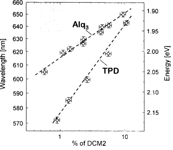
The work presented in this section has grown out of two recent reports by Bulovic et al describing spectral red shifts in the emission of amorphous organic thin films doped with the red laser dye DCM2 [12,13] (see Fig. 2.1 for chemical structures). By changing the concentration of DCM2 present in a film of

N,N'-diphenyl-N,N'-bis(3-methylphenyl)-[1,1'-biphenyl]-4,4'-diamine (TPD) from 0.9% to 11%, the peak electroluminescence emission wavelength was shifted from k=570 nm to k=645 nm (see Fig. 2.2). (For these measurements, the DCM2:TPD film comprised the active layer of an OLED.) Because DCM2 is a highly polar molecule (with

- 1 D in ground state), and TPD is nearly nonpolar (with p-I D in ground state), increasing the DCM2 concentration increases the strength of the local electric fields present in the film. This increase in the local fields was associated with the spectral shift. Similar results were also observed for DCM2 in Alq3. A subsequent report argued that the spectral shift is actually due to

a progressive increase in the presence of clustered dye molecules with increasing dye concentration [14]. In this case, the authors studied the electroluminescence of DCM2 in an OLED structure, and saw that increasing the DCM2 concentration was correlated to a decrease in the quantum efficiency of the device, which they attributed to the presence of an increase in the prevalence of aggregated dye molecules (see Fig. 2.3). Since aggregated dye molecules are generally thought to have red-shifted emission compared to the monomer, these authors correlated the red shift in photoluminescence of Alq3:DCM2 films to the decrease in

electroluminescent quantum efficiency as the DCM2 doping was increased, and concluded that red shifts simply reflected an increase in emission from aggregate states. We set out to clarify this issue, by developing an experiment that isolated the "solid-state solvation" effect described by Bulovic.

We performed photoluminescence measurements (using X=480 nm light) on films consisting of a polystyrene (PS) matrix, a small concentration of the laser dye DCM2, and a range of concentrations of the polar small molecule material camphoric anhydride (CA). (In these films, only the DCM2 molecules fluoresce upon excitation by k=480 nm light). The films were spun cast at 2000 rpm from solutions with a total concentration of 30 mg/mL. The

solutions were all made by first massing out polystyrene into a vial and then adding appropriate amounts of 20 mg/mL CA solution and 0.033 mg/mL DCM2 solution.

This material system was designed to allow us to keep the DCM2 concentration constant, and thereby fix DCM2 aggregation effects, while still modifying the dipole concentration of the film. We modified the dipole concentration by changing the concentration of CA, which has a large dipole moment (p-6D in ground state) relative to its molecular weight and is essentially optically inactive over the range of wavelengths relevant for studying the properties of DCM2. The polymer host material polystyrene was chosen because it provides a transparent, non-polar background for the system.

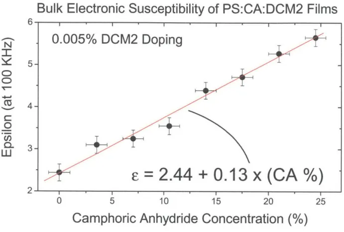
For a fixed DCM2 concentration of 0.005%, the DCM2 emission spectrum shifts continuously from 2.20 eV (563 nm) to 2.05 eV (605 nm) for CA concentrations ranging from 0% to 24.5% (see Figs. 2.4 and 2.5). (Chemical structures of CA and PS are shown in Figure 2.4.) These results show that large shifts in emission spectra can be observed in films that have negligible DCM2 aggregation. Furthermore, the spectral shift is clearly correlated with the increase in the concentration of polar molecules in the amorphous host thin film. While these results already make it difficult to support a theory that these spectral shifts involve the aggregation of DCM2 molecules, we also performed the same experiments with DCM2

concentrations up to 0.05%, and observed no change, again indicating that the concentration of DCM2, and therefore aggregation effects, do not contribute to the spectral shifts (at least for the low level DCM2 concentrations employed.)

These results would then tend to suggest a "solid state solvation" effect like the one presented by Bulovic. However, in that report, the physical mechanism for the spectral shifts is described only generally, in that it is related to the presence of significant local fields in the medium and that the local fields are due to the presence of dipolar molecules. We agree with

this assessment, so far as it goes, but it is necessary to take this analysis further if we are to evaluate quantitatively if such a mechanism makes sense.

2.3 Theory of Spectral Shifts due to Local Fields

As discussed in Section 1.6, the presence of local fields can modify the energy associated with a molecular transition. In this section we further develop the theory of the changes in the transition energy between an initial state Ii) and a final state If), where these wavefunctions

correspond to the molecule in the presence of zero field. In general, the changes to the transition energy come from two sources.

The first source comes from a direct modification by the local field of Ii) and If), which

implies a modification of the associated E, and Ef . If we describe the exact states and energies

in the presence of the field by i),

4,

due to this internal modification of the electronic structure, AEin, , is given by,

AEint ={Ef - (kf - ki

To determine the exact energies, E, and Ef, it is generally necessary to perform a full quantum mechanical calculation of the molecular energy levels in the presence of the field. Clearly this is not very desirable, because it makes it almost impossible to develop a straightforward

relationship between the external field and the change in transition energy. We will return to this difficulty below.

The second source comes from the electrostatic interaction between the molecular charge distributions of the initial and final states and the local field itself. This is the type of energy shift mentioned in Section 1.6. As indicated there, the change in the transition energy is just given by the difference between the electrostatic interaction energies in the two states (although in that expression a static local field was assumed, which is not the case here). If we identify the change in the transition energy due to electrostatic interactions by AEs , then we have,

where gp" (F) and q<'O (F) describe the potentials due to the local fields for the two states, and p (F) and pf (F) are the charge distributions for the two states. In a more complete treatment, one would determine the electrostatic interaction energies using the charge distributions due to

i) and but to simplify the analysis, we assume that I i) and

If)

molecule. In addition, we know that AEn =0, and so we only have to determine AE, .

To do this, we first obtain a simpler form for the charge distributions. For excitons, we are dealing with neutral molecules, in which case the dominant term of the multipolar expansion

of p(F) is the dipole moment. If we work within this dipole approximation, and note that the

electrostatic interaction energy between a dipole, j , and an electric field, F , is,

then we have that,

AEes= _{f- /)}

where j, and fif are just the dipoles associated with p

(F)

The first (and most straightforward) treatment of this problem is attributed to Onsager, who can be thought of as the originator to the continuum approximation. In short, Onsager recognized that one way to treat the field due to a collection of surrounding molecules was to

lump the surrounding molecules into a continuous medium characterized by a single parameter, the dielectric constant, E. In the Onsager model, therefore, the surrounding molecules form a homogeneous dielectric.

Since it is necessary to define a boundary between the medium and the molecule under study, Onsager proposed that the molecule exists within a spherical cavity of radius a , and that the charge distribution due to the molecule, in the dipole approximation, consists of an

appropriate point dipole located at the center of the cavity. In this model, the surrounding medium produces an electric field in response to the presence of a charge distribution in the

cavity (because the "medium" is just a dielectric), and for this reason, the resulting field is known as the reaction field. For a dipole of pi we find that the reaction field, FR , is given by,

- A..

a where

A = 2(c - 1)

2E +1

To illustrate the trends expected in FR as c changes, a plot of A over a range of e values is

shown in Figure 2.6. Note how the rise in A is steepest when c is smallest, indicated that even small changes in E can yield large changes in FR if E is moderately small to begin with.

In solutions, the solvent molecules are relatively free to move and reorient, and the simple dielectric description applies very well (in that the molecules typically have no intrinsic orientation, and freely rearrange themselves in the presence of a field). As a result, Ooshika, Lippert, and Mataga [15-17] subsequently applied the Onsager model to explain the shifts in absorption and emission spectra of dye molecules in solution. To follow their development we recall again the energy diagram used to explain the Franck-Condon shift, in Fig. 1.1. We recall that the difference between the absorption and emission energies is due to electronic transitions occuring much more quickly than the nuclear reorganization, and so the electronic transition occurs within a fixed nuclear framework. However, while nuclear reorganizations might be slow relative to electronic transitions, they are still fast compared to exciton lifetimes.

Now consider expanding our picture of the "system" to include the surrounding medium. In addition to the nuclear response to an electronic transition, we now have to consider a

response (due to the surrounding medium) to the change in the charge distribution on the molecule under study. If this response is to include molecular rearrangements, then clearly it must occur on a time scale slow compared to electronic transitions. It might even occur on a time scale slow compared to exciton relaxation, which would create a rather complicated problem. However, measurements have shown that typically the solvent response is still fast compared to the exciton lifetime. As a result, the reaction field due to the surrounding medium, just like the nuclear framework of the molecule itself, is fixed during an electronic transition.