HAL Id: hal-02046089
https://hal.archives-ouvertes.fr/hal-02046089
Preprint submitted on 22 Feb 2019
HAL is a multi-disciplinary open access
archive for the deposit and dissemination of
sci-entific research documents, whether they are
pub-lished or not. The documents may come from
teaching and research institutions in France or
L’archive ouverte pluridisciplinaire HAL, est
destinée au dépôt et à la diffusion de documents
scientifiques de niveau recherche, publiés ou non,
émanant des établissements d’enseignement et de
recherche français ou étrangers, des laboratoires
Parallel Controllability Methods For the Helmholtz
Equation
Marcus Grote, Frédéric Nataf, Jet Hoe Tang, Pierre-Henri Tournier
To cite this version:
Marcus Grote, Frédéric Nataf, Jet Hoe Tang, Pierre-Henri Tournier. Parallel Controllability Methods
For the Helmholtz Equation. 2019. �hal-02046089�
Parallel Controllability Methods
For the Helmholtz Equation
Marcus J. Grotea, Fr´ed´eric Natafb, Jet Hoe Tanga, Pierre-Henri Tournierb
aUniversity of Basel, Spiegelgasse 1, 4051 Basel, Switzerland
bLaboratoire J.L. Lions, Universit´e Pierre et Marie Curie, 4 place Jussieu, 75005 Paris,
France, and ALPINES INRIA, Paris, France
Abstract
The Helmholtz equation is notoriously difficult to solve with standard numerical methods, increasingly so, in fact, at higher frequencies. Controllability meth-ods instead transform the problem back to the time-domain, where they seek the time-harmonic solution of the corresponding time-dependent wave equa-tion. Two different approaches are considered here based either on the first or second-order formulation of the wave equation. Both are extended to gen-eral boundary-value problems governed by the Helmholtz equation and lead to robust and inherently parallel algorithms. Numerical results illustrate the accuracy, convergence and strong scalability of controllability methods for the solution of high frequency Helmholtz equations with up to a billion unknowns on massively parallel architectures.
Keywords: Helmholtz equation; time-harmonic scattering; exact
controllability; finite elements; domain decomposition; parallel scalability
1. Introduction
The efficient numerical solution of the Helmholtz equation is fundamental to the simulation of time-harmonic wave phenomena in acoustics, electromagnet-ics or elasticity. As the time frequency ω ą 0 increases, so does the size of the linear system resulting from any numerical discretization in order to resolve the 5
increasingly smaller wave lengths. With the increase in frequency, however, the performance of standard preconditioners based on multigrid, incomplete factor-ization or domain decomposition approaches, originally developed for positive definite Laplace-like equations, rapidly deteriorates [1].
In recent years, a growing number of increasingly sophisticated precondi-10
tioners has been proposed for the iterative solution of the Helmholtz equation;
Email addresses: marcus.grote@unibas.ch (Marcus J. Grote), nataf@ann.jussieu.fr (Fr´ed´eric Nataf), jet.tang@unibas.ch (Jet Hoe Tang), tournier@ljll.math.upmc.fr (Pierre-Henri Tournier)
”Shifted Laplacian” preconditioners [2], for instance, have led to modern multi-grid [3, 4] and domain decomposition preconditioners [5, 6]. While some of those preconditioners may achieve a desirable frequency independent conver-gence behavior in special situations [7], that optimal behavior is often lost in 15
the presence of strong heterogeneity. Moreover, they are typically tied to a special discretization or fail to achieve optimal scaling on parallel architectures. Controllability methods (CM) offer an alternative approach for the numerical solution of the Helmholtz equation. Instead of solving the problem directly in the frequency domain, we first transform it back to the time domain where we 20
seek the corresponding time-dependent periodic solution, yp¨, tq, with known period T “ 2π{ω. By minimizing an energy functional J pv0, v1q which penalizes
the mismatch after one period, controllability methods iteratively adjust the (unknown) initial condition pv0, v1q thereby steering yp¨, tq towards the desired
periodic solution. Once the minimizer of J has been found, we immediately 25
recover from it the solution of the Helmholtz equation. As the CM combines the numerical integration of the time-dependent wave equation with a conjugate gradient (CG) iteration, it is remarkably robust and inherently parallel.
In [8], Bristeau et al. proposed the first CM for sound-soft scattering prob-lems based on the wave equation in standard second-order form. Since the initial 30
condition pv0, v1q then lies in H1ˆL2, the original formulation requires the
solu-tion of a coercive elliptic problem at each CG iterasolu-tion. Heikkola et al. in [9, 10] presented a higher-order version by using spectral FE and the classical fourth-order Runge-Kutta (RK) method. For more general boundary-value problems, such as wave scattering from sound-hard obstacles, inclusions, or wave propaga-35
tion in physically bounded domains, the original CM will generally fail because the minimizer of J is no longer unique. In [11], we proposed alternative energy functionals which restore uniqueness, albeit at a small extra computational cost, for general boundary-value problems governed by the Helmholtz equation.
More recently, Glowinski and Rossi [12] proposed a CM based on the wave 40
equation in first-order (or mixed) form using classical Raviart-Thomas (RT) finite elements. As pv0, v1q then lies in L2ˆ pL2qd, the solution of an elliptic
problem at each CG iteration is no longer necessary and the CM becomes in principle trivially parallel. Still, the lack of availability of mass-lumping for RT elements again nullifies the main advantage of the first-order formulation 45
because the mass-matrix now needs to be ”inverted” at each time-step. Here we revisit the original CM from [8, 12] and consider two distinct dis-cretizations, which both lead to highly efficient and inherently parallel meth-ods. In Section 2, we recall the CMCG method based on the wave equation in second-order form and propose a filtering procedure which permits the use of 50
the original energy functional J , regardless of the boundary conditions. Next, in Section 3, we consider the CM based on the wave equation in first-order form and again show how to extend it to arbitrary boundary-value problems governed by the Helmholtz equation. Thanks to a recent hybrid discontinuous Galerkin (HDG) method [13], which automatically yields a block-diagonal mass-55
matrix, the time integration of the wave equation then becomes truly explicit and the entire CMCG approach trivially parallel. In Section 4, we perform a
series of numerical experiments to illustrate the accuracy, convergence behavior and inherent parallelism of the CMCG approach. In particular, we apply it to large-scale high-frequency Helmholtz problems with up to a billion unknowns 60
to demonstrate its strong scalability on massively parallel architectures. 2. Controllability methods for the second-order formulation 2.1. Time-harmonic waves
We consider a time-harmonic wave field upxq in a bounded connected com-putational domain Ω Ă Rd, d ď 3, with a Lipschitz boundary Γ. The boundary
consists of three disjoint components, Γ “ ΓDY ΓN Y ΓS where we impose
a Dirichlet, Neumann and impedance (or Sommerfeld-like absorbing) bound-ary condition, respectively; the boundbound-ary condition is omitted whenever the corresponding component is empty. In Ω, the wave field u hence satisfies the Helmholtz equation
´∆upxq ´ k2pxq upxq “ f pxq, x P Ω, (2.1a) Bupxq
Bn ´ ikpxq upxq “ gSpxq, x P ΓS, (2.1b) Bupxq
Bn “ gNpxq, x P ΓN, (2.1c) upxq “ gDpxq, x P ΓD, (2.1d)
where ω ą 0 is the (angular) frequency, cpxq ą 0 the wave speed, kpxq “ ω{cpxq the wave number, n the unit outward normal, and f , gN, gS and gDare known
65
and may vanish.
The above formulation is rather general and encompasses most common applications such as sound-soft scattering problems with ΓS ‰ H and ΓD ‰
H, sound-hard scattering problems with ΓS ‰ H and ΓN ‰ H, or physically
bounded domains with ΓS “ H. We shall always assume for any particular
70
choice of ω, cpxq, or combination of boundary conditions that (2.1) is well-posed and has a unique solution u P H1pΩq.
Instead of solving the Helmholtz equation directly in the frequency domain, we now reformulate (2.1) in the time domain. Then, the corresponding time-harmonic wave field, Re upxq e´iωt(, satisfies the (real-valued) time-dependent
wave equation 1 c2pxq B2ypx, tq B2t ´ ∆ypx, tq “ Re fpxq e ´iωt( , x P Ω, t ą 0, (2.2a) Bypx, tq Bn ` 1 cpxq Bypx, tq Bt “ Re gSpxq e ´iωt( , x P Γ S, t ą 0, (2.2b) Bypx, tq Bn “ Re gNpxq e ´iωt( , x P Γ N, t ą 0, (2.2c) ypx, tq “ Re gDpxq e´iωt( , x P ΓD, t ą 0, (2.2d) ypx, 0q “ v0pxq, Bypx, 0q Bt “ v1pxq, x P Ω, (2.2e)
for the (unknown) initial values v0“ Re tuu and v1“ ω Im tuu.
For sound-soft scattering problems (2.1), where |ΓD| ą 0 and |ΓS| ą 0,
Bris-teau et al. [8, 14] proposed to determine upxq via controllability by computing a time-periodic solution ypx, tq of (2.2) with period T “ 2π{ω. Once the initial values v0, v1 of y are known, the solution u of the original Helmholtz equation
(2.1) is immediately given by u “ v0` i ωv1, v0, v1P H 1 pΩq. (2.3)
To determine v0 and v1, the problem is reformulated as a least-squares
opti-mization problem over H1
pΩq ˆ L2pΩq for the quadratic cost functional
J pv0, v1q “ 1 2 ż Ω |∇ypx, T q´∇v0pxq|2dx` 1 2 ż Ω 1 c2pxqpytpx, T q´v1pxqq 2dx, (2.4)
where y satisfies (2.2) with the initial values v0 and v1. The functional J
mea-sures in the energy norm the mismatch between the solution of (2.2) at the initial 75
time and after one period. It is non-negative and convex, while J pv0, v1q “ 0
if, and only if, ∇yp¨, T q “ ∇yp¨, 0q and ytp¨, T q “ ytp¨, 0q for any given initial
values pv0, v1q; in particular, J pv0, v1q “ 0 if v0“ Re tuu and v1“ ω Im tuu.
For more general scattering problems, however, J is no longer strictly convex as the T -periodicity of ytand ∇y no longer guarantees a unique periodic solution
80
y of (2.2). Instead, for the general boundary-value problem (2.1), the situation is more complicated and summarized in the following theorem [11] .
Theorem 1. Let u P H1
pΩq be the unique solution of (2.1) and y P C0pr0, T s; H1pΩqqX C1
pr0, T s; L2pΩqq be a (real-valued) solution of (2.2) with initial values pv0, v1q P
H1
pΩq ˆ L2pΩq. If ∇y and yt are time periodic with period T “ 2π{ω, then y
admits the Fourier series representation
pyp¨, tq, ϕq “ pRe u e´iωt( , ϕq ` pλ ` ηt, ϕq ` ÿ
|`|ą1
pγ`eiω`t, ϕq (2.5)
for any ϕ P H1
D, where the constants λ, η P R and the eigenfunctions γ` “
α`` iβ`, α`, β`P H1pΩq, |`| ą 1 satisfy ´∆γ`pxq ´ p`kpxqq2γ`pxq “ 0, x P Ω, (2.6a) Bγ`pxq Bn ` i`kpxq γ`pxq “ 0, x P ΓS, (2.6b) Bγ`pxq Bn “ 0, x P ΓN, (2.6c) γ`pxq “ 0, x P ΓD, (2.6d)
Let v “ v0` pi{ωq v1. Then v satisfies
pv, ϕq “ pu, ϕq ` pλ ` i ωη, ϕq `
ÿ
|`|ą1
Furthermore, if |ΓS| ą 0, then η “ 0. If |ΓD| ą 0, then λ “ η “ 0.
Here HD1 :“ tw P H1pΩq : w “ 0 on ΓDu and p¨, ¨q denotes the standard L2pΩq
inner product. 85
Proof. See [11].
For sound-soft scattering problems (|ΓS| ą 0, |ΓD| ą 0), where both Dirichlet
and Sommerfeld-like absorbing boundary conditions are imposed on Γ, all the eigenfunctions γ`, |`| ą 1, and the constants λ, η in (2.7) vanish identically.
Thus, the minimizer v “ v0` pi{ωqv1 of J in (2.4) then coincides with u.
90
For scattering problems from sound-hard obstacles or penetrable inclusions (|ΓS| ą 0, |ΓD| “ 0), the eigenfunctions γ` and the constant η in (2.7) still
vanish identically, yet the constant λ may be nonzero. Given any minimizer v “ u ` λ of J , we can recover u by subtracting the spurious shift λ using the compatibility condition: λ “ 1 }k}2L2pΩq` i|k|L1pΓ Sq ˆ ż Ω k2v ` i ż ΓS kv ` ż Ω f ` ż ΓS gS` ż ΓN gN ˙ .
In fact, any impedance condition (2.1b) that includes a positive (or negative) definite zeroth order term, such as a more accurate absorbing boundary condi-tion [15, 16], also circumvents the indeterminacy due to λ.
For wave propagation in physically bounded domains (|ΓS| “ 0), the
eigen-functions γ` and the constants λ, η in (2.7) typically do not vanish. However,
95
we can always restore uniqueness by replacing J with an alternative energy functional, thereby incurring a small increase in computational cost – see [11]. 2.2. Fundamental frequency extraction via filtering
From Theorem 1 we conclude that a minimizer of J generally yields a time-dependent solution y of (2.2), which contains a constant shift determined by 100
λ, a linearly growing part determined by η, and higher frequency harmonics determined by γ`, all superimposed on the desired time-harmonic field u with
fundamental frequency ω. Those spurious modes can be eliminated by replacing J with an alternative energy functional at a small extra computational cost [11]. Instead we now propose an alternative approach via filtering which removes all 105
spurious modes without requiring a modified energy functional.
Let ypx, tq be the time-dependent solution of (2.2) that corresponds to a minimizer pv0, v1q of J . Next, we definey P tw P Hp
1 pΩq | w “ gD on ΓDu as p ypxq :“ 1 T żT 0 `ypx, tq ` i ωytpx, tq˘ e iωt dt. (2.8)
To extract upxq from ypx, tq, we now take advantage of the mutual orthogonality of different time harmonics exppiω`tq in L2
eiωt and integrate in time over p0, T q to obtain p ypxq “ 1 T żT 0 ` Retu e´iωt
u ` λ ` ηt ` i Imtu e´iωtu `iη ω˘ e iωtdt “ 1 T żT 0
u e´iωteiωtdt ´iη
ω “ u ´ iη ω. (2.9) This yields upxq “ypxq `p iη ω, x P Ω (2.10)
where λ and all γ` have vanished but the constant η is still undetermined.
If |ΓS| ą 0 or |ΓD| ą 0, Theorem 1 implies that η “ 0 and thus upxq “ypxq.p Otherwise in the pure Neumann case (Γ “ ΓN), we determine η by integrating
(2.10), multiplied by k2
pxq, over Ω and using the compatibility condition ´ ż Ω k2pxqupxq dx “ ż Ω f pxq dx ` ż BΩ gNpxq ds. (2.11)
from (2.1a). This immediately yields the remaining constant iη ω “ ´ 1 }k}2L2pΩq ˆ ż Ω f pxq dx ` ż BΩ gNpxq ds ` ż Ω k2pxqypxqdxp ˙ . (2.12) We summarize the above derivation in the following proposition.
Proposition 1. Let u P H1
pΩq be the unique solution of (2.1) and y the time dependent solution of (2.2) corresponding to a minimizer pv0, v1q P H1pΩq ˆ
110 L2
pΩq of J , i.e. J pv0, v1q “ 0. Then u is given by (2.10) with η “ 0 if |ΓS| ą 0
or |ΓD| ą 0, and with η given by (2.12) when ΓN “ BΩ.
Not only does the above filtering approach allow us to use the original cost functional J , it also involves a negligible computational effort or storage amount, as the time integral fory can be calculated cumulatively via numerical quadra-p 115
ture during the solution of the wave equation (2.2). 2.3. The CMCG Algorithm
To minimize the quadratic cost functional J defined by (2.4) over H1pΩq ˆ L2pΩq, a natural choice is the conjugate gradient (CG) method [8], which re-quires the Fr´echet derivative of J at v “ pv0, v1q:
120 xJ1pvq, δvy “ ´ ż Ω ∇pypx, T q ´ v0pxqq ¨ ∇δv0pxq dx (2.13) ´ ż Ω 1 c2pxqpytpx, T q ´ v1pxqqδv1pxq dx ` ż Ω 1 c2pxq`ppx, 0qδv1pxq ´ ptpx, 0qδv0pxqq dx (2.14) ` ż ΓS 1 cpxq ppx, 0qδv0pxq ds.
Here δv “ pδv0, δv1q denotes an arbitrary perturbation, x¨, ¨y the standard
du-ality pairing, and p the solution of the adjoint (backward) wave equation: 1 c2pxq B2 B2tppx, tq ´ ∆ppx, tq “ 0, x P Ω, t ą 0, (2.15a) Bppx, tq Bn ´ 1 c B Btppx, tq “ 0, x P ΓS, t ą 0 (2.15b) Bppx, tq Bn “ 0, x P ΓN, t ą 0, (2.15c) ppx, tq “ 0, x P ΓD, t ą 0, (2.15d) ppx, T q “ p0pxq, Bppx, T q Bt “ p1pxq, x P Ω, (2.15e)
and the initial conditions satisfy for any w P H1 DpΩq p0pxq “ ytpx, T q ´ v1pxq, x P Ω, ż Ω p1pxq c2pxqwpxq dx “ ż ΓS p0pxq cpxqwpxq ds ´ ż Ω ∇pypx, T q ´ v0pxqq ¨ ∇wpxq dx.
The derivation of (2.13) and (2.15) can be found in [8]. In each CG iteration the derivative J1pvq requires the solution of the forward and backward (adjoint)
wave equations (2.2) and (2.15) over one period r0, T s. Moreover, each CG iteration requires an explicit (Riesz) representer ˜g “ p˜g0, ˜g1q P HD1pΩq ˆ L2pΩq
of the gradient g “ pg0, g1q “ J1pvq defined in (2.13), which is determined by
solving the symmetric and coercive elliptic problem [8, 17]: p∇˜g0, ∇ϕq “ ż Ω g0pxqϕpxq dx “ ż Ω ∇pv0pxq ´ ypx, T qq ¨ ∇ϕpxq ´ 1 c2pxqptpx, 0qϕpxq dx ` ż ΓS 1 cpxq ppx, 0qϕpxq ds, @ϕ P H 1 D, (2.16a) ˜ g1 “ g1 “ v1´ ytp¨, T q ` c´2pp¨, 0q. (2.16b)
For the sake of completeness, we list the full CMCG Algorithm – see [8, 11]: CMCG Algorithm.
(1) Initialize vp0q “ pvp0q 0 , v
p0q
1 q (initial guess).
(2) Solve the forward and the backward wave equations (2.2) and (2.15) to de-termine the gradient of J , gp0q“ J1pvp0qq, defined by (2.13).
125
(3) Solve the coercive elliptic problem (2.16) with g “ gp0q to determine the new
search direction ˜gp0q.
(4) Set rp0q“ dp0q “ ˜gp0q.
(5) For ` “ 1, 2, . . .
5.1 Solve the wave equation (2.2) with f “ gD “ gS “ gN “ 0 and the
130
initial values dp`q“ pdp`q 0 , d
p`q
1 q and the backward wave equation (2.15).
5.2 Solve the coercive elliptic problem (2.16) with g “ gp`q to get ˜gp`q. 5.3 α`“ } ∇r0p`q}2L2pΩq` }p1{cq r p`q 1 } 2 L2pΩq p ∇˜gp`q0 , ∇dp`q0 qL2pΩq` pp1{c2q ˜gp`q1 , dp`q1 qL2pΩq 5.4 vp``1q“ vp`q´ α `dp`q 135 5.5 rp``1q“ rp`q´ α `˜gp`q 5.6 β`“ }∇rp``1q0 }2L2pΩq` }p1{cq r p``1q 1 }2L2pΩq }∇r0p`q}2L2pΩq` }p1{cq r p`q 1 }2L2pΩq 5.7 dp``1q“ rp``1q` β `dp`q
5.8 Stop when the relative residual lies below the given tolerance tol g f f e }∇rp``1q0 }2L2pΩq` }p1{cq r p``1q 1 } 2 L2pΩq }∇rp0q0 }2L2pΩq` }p1{cq r p0q 1 }2L2pΩq ď tol.
(6) Return approximate solution uh of (2.1) given by
uh“ vp`q0 `
i ωv
p`q 1 .
Since ˜g0 P H1pΩq, the updates of rpkq0 , d pkq 0 and v
pkq
0 in Steps 5.4, 5.5 and
5.7 in the CMCG Algorithm also remain in H1
pΩq. We emphasize that (2.16a) 140
is independent of ω and leads to a symmetric and positive definite linear sys-tem, which can be solved efficiently and in parallel with standard numerical (multigrid, domain decomposition, etc.) methods [18, 6].
3. Controllability methods for first-order formulations
The CMCG Algorithm from Section 2.3 iterates on the initial value pv0, v1q P
145 H1
pΩq ˆ L2pΩq of the secondorder wave equation (2.2) until its solution is T -time periodic. However, the gradient of the cost functional J pv0, v1q, which is
needed during the CG update, only lies in the dual space H´1
pΩq ˆ L2pΩq. To ensure that the solution remains sufficiently regular and in H1pΩq ˆ L2pΩq, the corresponding Riesz representative is computed at every CG iteration by 150
solving the strongly elliptic problem (2.16a). In [12], Glowinski et al. derived an equivalent first-order formulation for sound-soft scattering problems, where the solution instead lies in pL2pΩqqd`1, which is reflexive. As a consequence, all CG iterates automatically lie in the correct solution space pL2
pΩqqd`1, while the solution of (2.16a) is no longer needed.
155
3.1. First-order formulation for general boundary conditions
Again, we always assume for any particular choice of ω, cpxq, f and com-bination of boundary conditions that (2.1) has a unique solution u P H1pΩq.
Following [12], we now let v “ yt, p “ ∇y and rewrite the time-dependent wave
equation (2.2) in first-order form: 1 c2pxqvtpx, tq ´ ∇ ¨ ppx, tq “ Re fpxq e ´iωt( , x P Ω, t ą 0, (3.1a) B Btppx, tq “ ∇vpx, tq, x P Ω, t ą 0, (3.1b) ppx, tq ¨ n ` 1 cpxqvpx, tq “ Re gSpxq e ´iωt( , x P ΓS, t ą 0, (3.1c) ppx, tq ¨ n “ Re gNpxq e´iωt( , x P ΓN, t ą 0, (3.1d)
vpx, tq “ Re ´iωgDpxq e´iωt( , x P ΓD, t ą 0 (3.1e)
with the initial conditions
ppx, 0q “ p0pxq P Rd, vpx, 0q “ v0pxq P R, x P Ω. (3.1f)
Hence, the solution pp, vq of (3.1) lies in the function space Q [19, 20], Q “ C0
pr0, T s; Hpdiv; Ωq ˆ L2pΩqq X C1pr0, T s; pL2pΩqqd`1q. (3.2) In terms of p and v, the energy functional J defined in (2.4) now becomes
p J pp0, v0q “ 1 2 ż Ω |ppx, T q ´ p0pxq|2dx ` 1 2 ż Ω 1 c2pxqpvpx, T q ´ v0pxqq 2 dx, (3.3)
where pp, vq solves (3.1) with initial value pp0, v0q P Hpdiv; Ωq ˆ L2pΩq.
The CMCG Algorithm for the first-order formulation is identical to that for the second-order formulation from Section 2.3 except for Steps 2 and 5.1, where J1 is now replaced by pJ1: x pJ1 pp0, v0q, pδp0, δv0qy “ ż Ω pp˚px, 0q ´ p˚px, T qqδp0pxq dx (3.4) ` ż Ω pv˚px, 0q ´ v˚px, T qqδv0pxq dx.
Here pδp0, δv0q P P ˆ L2pΩq denotes an arbitrary perturbation with
P “ tp P Hpdiv; Ωq | p ¨ n “ 0 on ΓNu, (3.5)
whereas pp˚, v˚q P P ˆ L2
pΩq solves the backward (adjoint) wave equation in first-order form [12], that is (3.1) with f ” gS ” gN ” gD” 0 and
p˚
p¨, T q “ pp¨, T q ´ p0, v˚p¨, T q “ vp¨, T q ´ v0.
For sound-soft scattering problems (|ΓD|, |ΓS| ą 0), the functional pJ always
has a unique (global) minimizer, which therefore coincides with the (unique) time-harmonic solution Re upxq e´iωt(
of (3.1). For more general boundary 160
value problems, however, the minimizer of pJ is not necessarily unique, as shown in the following theorem.
Theorem 2. Let u P H1pΩq be the unique solution of (2.1) and pp, vq P Q be a real-valued solution of (3.1) with initial values pp0, v0q P Hpdiv; Ωq ˆ L2pΩq. If
p and v are time periodic with period T “ 2π{ω, then p and v admit the Fourier series representation pp¨, tq “ Re ∇u e´iωt( ` λ ` 8 ÿ |`|ą1 γp`e´iω`t, (3.6a) vp¨, tq “ ω Im u e´iωt( ` η ` 8 ÿ |`|ą1 γ`ve´iω`t, (3.6b)
where the constant η P R, λ P P with ż
Ω
λ ¨ ∇ϕ dx “ 0, @ϕ P H1pΩq, ϕ|ΓD ” 0, (3.7)
and the complex-valued eigenfunctions γp` P P, γ`vP L2pΩq, |`| ą 1 satisfy
´c2pxq∇ ¨ γp`pxq ` iω`γ`vpxq “ 0, x P Ω, (3.8a) iω`γp`pxq “ ∇γ`vpxq, x P Ω, (3.8b) cpxqγp`pxq ¨ n ` γ v `pxq “ 0, x P ΓS, (3.8c) γp`pxq ¨ n “ 0, x P ΓN, (3.8d) γ`vpxq “ 0, x P ΓD. (3.8e) Furthermore, if |ΓSY ΓD| ą 0, then η “ 0. Proof. Let
qp¨, tq “ pp¨, tq ´ Re ∇u e´iωt( , wp¨, tq “ vp¨, tq ´ ω Im u e´iωt( .
Then w and q satisfy (3.1) with f ” gD” gS ” gN ” 0 and initial values
qpx, 0q “ p0pxq ´ Re t∇upxqu , wpx, 0q “ v0pxq ´ ω Im tupxqu , x P Ω.
Since p and v are T -periodic, so are q and w. Moreover, the mappings t ÞÑ pqp¨, tq, ψq, t ÞÑ pwp¨, tq, ϕq
are T -periodic and continuous for any pψ, ϕq P P ˆ L2pΩq [19]. Hence, they admit the Fourier series representation,
pqp¨, tq, ψq “ 8 ÿ `“´8 p γp`eiω`t, pwp¨, tq, ϕq “ 8 ÿ `“´8 p γ`veiω`t, where γp` P Cd, p γv ` P C. Next, we define γp`pxq “ 1 T żT 0 qpx, tq e´iω`tdt, γ`vpxq “ 1 T żT 0 wpx, tq e´iω`t dt, (3.9)
which implies that p γp` “ pγp`, ψq, pγ v ` “ pγ v `, ϕq.
We shall now show that γp` and γ`v satisfy (3.8) for all |`| ě 1. First, inte-gration by parts, (3.1a)-(3.1b) and the periodicity of q and w imply
γ`vpxq “ 1 T żT 0 wtpx, tq e´iω`t iω` dt ´ wpx, tq e´iω`t iω`T ˇ ˇ ˇ ˇ T 0 “ 1 T żT 0 c2pxq∇ ¨ qpx, tqe ´iω`t iω` dt, γp`pxq “ 1 T żT 0 qtpx, tq e´iω`t iω` dt ´ qpx, tq e´iω`t iω`T ˇ ˇ ˇ ˇ T 0 “ 1 T żT 0 ∇wpx, tqe ´iω`t iω` dt. Together with definition (3.9) of γp` and γv
`, we thus immediately obtain
iω`γ`v´ c2∇ ¨ γp` “ 0, iω`γp` “ ∇γ`v in Ω.
Since wpx, tq “ 0 for x P ΓD, we infer from (3.9) that
ż ΓD γv`pxqϕpxq ds “ 1 T żT 0 ż ΓD wpx, tqϕpxq ds e´iω`t dt “ 0, ϕ P L2 pΓDq, and hence γv
` satisfies (3.8e). Similarly, (3.8c), (3.8d) follow from the fact that
q and w satisfy (3.1c), (3.1d) with gN ” gS ” 0. Hence γ p `, γ
v
` satisfy (3.8) for
165
all |`| ě 1. In fact for ` “ 1, (3.8) corresponds to (2.1) in first-order formulation with γp1 “ ∇u, γ1v “ iωu, homogeneous boundary conditions and no sources.
By uniqueness, γp1and γv
1, together with their complex conjugates, are therefore
identically zero.
Next, we consider γp0, γv
0. Again, since q and w satisfy (3.1a)-(3.1e) with
f “ 0 and homogeneous boundary conditions, we obtain from (3.9) with ` “ 0 and the periodicity of q and w
ż Ω p∇ ¨ γp0q ϕ dx “ 1 T żT 0 ż Ω 1 c2wtϕ dxdt “ 0, @ϕ P L 2 pΩq, (3.10) ż Ω γ0v∇ ¨ ψ dx “ 1 T żT 0 ż Ω qt¨ ψ dxdt ´ 1 T żT 0 ż ΓS w ψ ¨ n dsdt (3.11) “ 1 T żT 0 ż ΓS c q ¨ n ψ ¨ n dsdt “ ż ΓS c γp0¨ n ψ ¨ n ds, @ψ P P.
In particular, (3.10)-(3.11) implies with ϕ “ γ0v and ψ “ γ p 0that ż ΓS c|γp0¨ n| 2 ds “ 0,
and hence, γp0¨ n “ 0 on ΓS, since c ą 0. Moreover, Green’s formula, together
with (3.10) and the homogeneous boundary conditions, implies that ż Ω γp0¨ ∇ϕ dx “ ´ ż Ω p∇ ¨ γp0q ϕ dx ` ż BΩ γp0¨ n ϕ ds “ 0, @ϕ P H1pΩq, ϕ|ΓD ” 0,
and therefore λ “ γp0 satisfies (3.7).
170
To show that γ0vis constant, we now let ϕ P C8
c pΩq and ψ “ ejϕ P Hpdiv; Ωq,
j “ 1, . . . , d, where ej is the j-th unit basis vector of Rd. Integration of (3.1b)
over r0, T s, definition (3.9) with ` “ 0 and the periodicity of q then yield 0 “ 1 T żT 0 ż Ω qtψ dxdt “ ´ 1 T żT 0 ż Ω w ∇ ¨ ψ dxdt “ ´ ż Ω γ0v Bϕ Bxj dx. (3.12) From (3.12), we conclude that Bxjγ
v
0 “ 0, j “ 1, . . . , d, which implies
γ0vpxq ” η, γ0vP H1pΩq.
Since γ0v satisfies (3.1e) with ` “ 0, η “ γ0v “ 0, if |ΓD| ą 0. Similarly, if
|ΓS ą 0|, (3.1c), together with γ p 0¨ n “ 0 on ΓS, yields 0 “ 1 T żT 0 “cpxqqpx, tq ¨ n ` wpx, tq‰ dt “ cpxqγp 0pxq ¨ n ` γ v 0pxq “ η, x P ΓS.
Thus, η “ 0 when |ΓDY ΓS| ą 0, which completes the proof.
For sound-soft scattering problems, where |ΓD| ą 0 and |ΓS| ą 0, η “ 0 and
all eigenfunctions γp`, γ`v, |`| ą 1 of (3.8) trivially vanish in (3.6) [21]. Therefore, (3.6)-(3.7) in Theorem 2 with t “ 0 imply that
175
pp0, ∇ϕq “ pRe t∇uu , ∇ϕq, ϕ P H1pΩq, ϕ|ΓD “ 0, v0 “ ω Im tuu .
From the real part of (2.1) we than conclude that
u “ ´k´2` Re tfu ` ∇ ¨ p0q ` iω´1v0. (3.13)
3.2. Fundamental frequency filtering for first-order formulation
When the CMCG method is applied to the first-order formulation (3.1), any minimizer of pJ pp0, v0q “ 0 generally consists of spurious perturbations η, λ
and eigenfunctions γp`, γ`v superimposed on the desired (unique) solution u of (2.1). To extract u from pp0, v0q, we apply a filtering approach, similar to that
in Section 2.2, and thereby restore uniqueness. Again, we multiply the Fourier series representation in (3.6) of v by eiωtand integrate over p0, T q. Since η and
λ are independent of time, while eiωtis orthogonal to eiω`t, |`| ą 1, all spurious
modes vanish and the resulting expression simplifies to: 2 T żT 0 vp¨, tq eiωt dt “ 2 T żT 0
Re ´iωu e´iωt( eiωt dt “ ´iωu,
which immediately yields
upxq “ 2i T ω
żT 0
vp¨, tq eiωt dt. (3.14)
We summarize this result in the following proposition.
Proposition 2. Let u P H1pΩq be the unique solution of (2.1) and pp, vq P Q
3.3. Hybrid DG FE-Discretization 180
In [12], Glowinski et al. used standard Raviart-Thomas (RT) finite ele-ments to discretize (3.1). Since no mass-lumping is available for RT eleele-ments on triangles or tetrahedra [22], each time-step then requires the inversion of the mass-matrix. To avoid that extra computational cost, which strongly impedes parallelization, we instead consider the recent hybrid discontinuous Galerkin 185
(HDG) FEM [13] to discretize (2.1) in its corresponding first-order formula-tion together with (3.1). Then, the mass-matrix is block-diagonal, with (small and constant) block size equal to the number of dof’s per element, so that the time-stepping scheme becomes truly explicit and inherently parallel.
Let Th denote a regular triangulation of Ωh, Eh the set of all faces and Pr
the space of polynomials of degree r. In addition, we define
Ph “ tr P pL2pΩqqd: r|K P pPrpKqqd, @K P Thu, (3.15)
Vh “ tw P L2pΩq : w|KP PrpKq, @K P Thu, (3.16)
Mh “ tµ P L2pEhq : µ|F P PrpF q, @F P Ehu. (3.17)
Following [13], the HDG Galerkin FE formulation reads: Find pph, vh,pvhq P Phˆ Vhˆ Mh such that
`Bph Bt , r ˘ K “ ´ pvh, ∇ ¨ rqK` xpvh, r ¨ nyBK, (3.18a) ` 1 c Bvh Bt , w ˘ K “ pf, wqK´ pph, ∇wqK` xpph¨ n, wyBK, (3.18b) xpph¨ n ` 1
cpvh, µyBKXΓS “ xRe tgSexpp´iωtqu , µyBKXΓS, (3.18c) xpph¨ n, µyBKXΓN “ xRe tgNexpp´iωtqu , µyBKXΓN, (3.18d) xpvh, µyBKXΓD “ xω Im tgDexpp´iωtqu , µyBKXΓD, (3.18e) for all pr, w, µq P Phˆ Vhˆ Mh, K P Thand t P r0, T s, where p¨, ¨qK and x¨, ¨yD
denote the L2-inner product on K or D, respectively and the numerical flux is
p
ph¨ n “ ph¨ n ´ τ pvh´pvhq on BK (3.18f) with the stabilization function τ from [13]. In addition, pph, vhq satisfies the
initial conditions
phpx, 0q “ p0pxq, vhpx, 0q “ v0pxq, x P Ω. (3.18g)
For the time integration of (3.18), we use the standard explicit fourth-order 190
Runge-Kutta (RK4) method.
3.4. Convergence and superconvergence
For a FE discretization with piecewise polynomials of degree r, we usually expect convergence as Ophr`1q with respect to the L2-norm. For the above
HDG discretization, however, an extra power in h can be achieved by applying 195
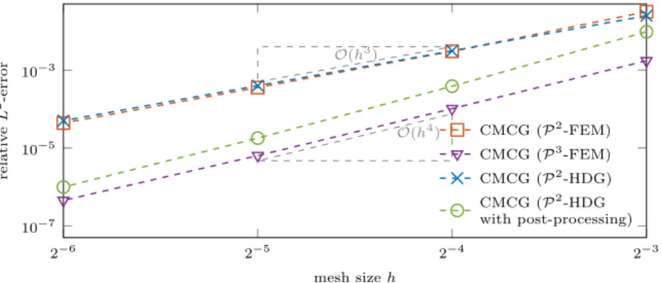
2´6 2´5 2´4 2´3 10´7 10´5 10´3 Oph3q Oph4q mesh size h relativ e L 2-error CMCG (P2-FEM) CMCG (P3-FEM) CMCG (P2-HDG) CMCG (P2-HDG with post-processing)
Figure 1: Convergence and superconvergence: the numerical error }u ´ uh} vs. mesh size
h “ 2´i, i “ 3, . . . , 6, obtained with the CMCG method for the second-order formulation
with P2-/P3-FE or for the first-order formulation with P2-HDG discretization, either with
or without post-processing.
a cheap local post-processing step [13]. The same (super-) convergence in space of order r ` 2 using only Pr-FE can be achieved with the CMCG method by
applying the post-processing step to the numerical solutions ppnT
h , v nT
h q of (3.1)
at the final time T “ nT∆t.
Let ppm h, v
m h, ˆv
m
hq denotes the fully discrete solution of (3.18) at tm“ m∆t.
First, we compute the new (more accurate) approximation pnT,˚
h of pp¨, T q by
solving the local problem ppnT,˚
h , ψqL2pKq “ ´pvhnT, ∇ ¨ ψqL2pKq` xpvnhT, ψ ¨ nyBK, @ψ P Ph on each K P Th. Then, we calculate the additional approximations yhnT,˚ of
yp¨, T q “ Retupxqu given by (3.13), vnT,˚
h of vp¨, T q in Pr`1pKq, which satisfy p∇ynT,˚ h , ∇ϕqL2pKq “ pphnT, ∇ϕqL2pKq, @ϕ P Pr`1pKq, pynT,˚ h , 1qL2pKq “ pyhnT, 1qL2pKq, p∇vnT,˚ h , ∇ϕqL2pKq “ pphnT,˚, ∇ϕqL2pKq, @ϕ P Pr`1pKq, pvnT,˚ h , 1qL2pKq “ pvhnT, 1qL2pKq,
for any element K P Th. The new approximate solution u is then given by (3.14)
200
with p and v replaced by pnT,˚
h and v nT,˚
h .
To illustrate the accuracy and verify the expected convergence rates for the various FE discretizations in the CMCG method, we now consider the following one-dimensional solution
upxq “ ´ exppikxq
of (2.1) in Ω “ p0, 1q with c “ 1, k “ 5π{4, ΓD “ t0u and ΓS “ t1u. Figure 1
shows the error }u ´ uh} obtained with the CMCG method for the first-order
formulation (2.2) and a P2-HDG discretization on a sequence of increasingly
finer meshes h “ 2´i, i “ 3, . . . , 6. Clearly as we refine the mesh, we always
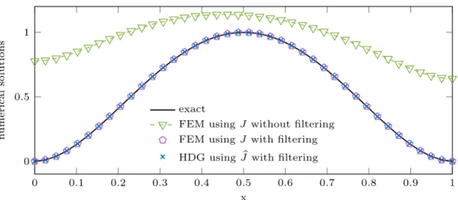
0 0.1 0.2 0.3 0.4 0.5 0.6 0.7 0.8 0.9 1 0 0.5 1 x n umerical solutions exact
FEM using J without filtering FEM using J with filtering HDG using pJ with filtering
Figure 2: Physically bounded domain: comparison of the exact solution u of (2.1) with the numerical solutions uhobtained with the CMCG method either applied to the second-order
formulation with standard FEM or to the first-order formulation with an HDG discretization.
reduce the time-step in the RK4 method to satisfy the CFL stability condition. The CG iteration stops once the tolerance tol “ 10´12 is reached. We also
compare the solutions obtained with the CMCG method applied to the second-order formulation using a (continuous) P2or P3-FEM. All numerical solutions
display the expected optimal convergence of order r ` 1 with polynomials of 210
degree r, while the first-order HDG approach even achieves superconvergence of order r ` 2, once local post-processing is applied to the final CG iterate. 3.5. Physically bounded domain
In the absence of Dirichlet or impedance boundary conditions, the first-order formulation does not yield the correct minimizer of J . As a simple remedy, we proposed in Section 3.2 a filtering procedure which removes the unwanted spurious modes. To illustrate the effectiveness of the filtering procedure, we now consider the exact solution of (2.1)
upxq “ 16x2px ´ 1q2 (3.20)
in Ω “ p0, 1q with homogeneous Neumann boundary conditions and k “ ω “ π{4, c “ 1. Note that k2is not an eigenvalue of (2.6) and therefore the solution
215
of (2.1) is well-posed. However, as p4kq2
“ π2 indeed corresponds to the first eigenvalue of the negative Laplacian, the CMCG method in general will not yield the correct (unique) solution – see Theorems 1 and 2. Indeed as shown in Figure 2, the original CMCG method [8] applied to the second-order formulation with the energy functional J in (2.4) does not yield the exact solution of (2.1), 220
unlike the numerical solutions obtained after filtering – see Sections 2.2 and 3.2.
4. Numerical results
Here we present a series of numerical examples that illustrate the accuracy, convergence behavior and parallel performance of the CMCG method. First, we
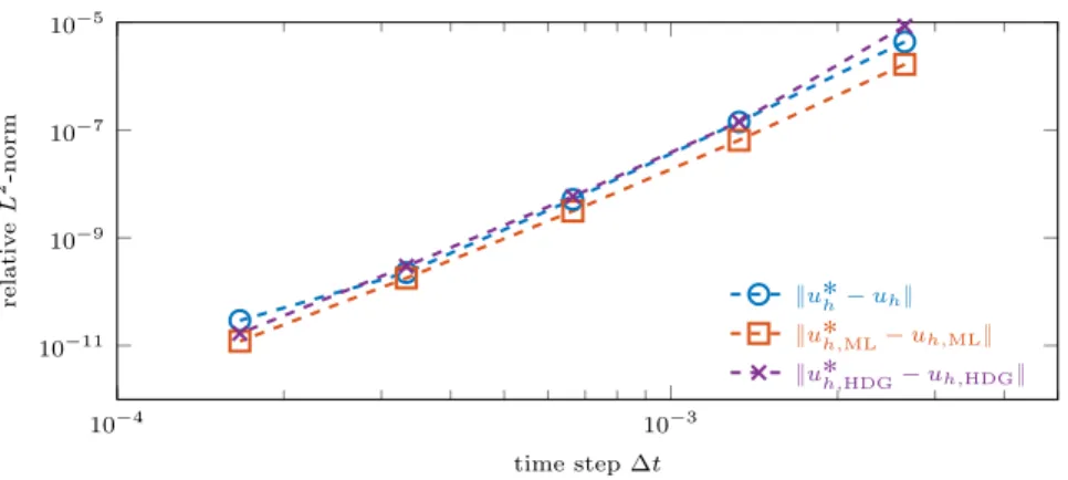
10´4 10´3 10´11 10´9 10´7 10´5 time step ∆t relativ e L 2-norm }u˚h´ uh} }u˚h,ML´ uh,ML} }u˚h,HDG´ uh,HDG}
Figure 3: Semi-discrete convergence: Comparison of the numerical solution uh, obtained
with the CMCG method, and u˚
h, obtained with a direct solver for the same fixed P2-FE
discretization (H1-conforming or HDG), both either with or without mass-lumping (ML)
verify that the numerical solution uhof (2.1) obtained with the CMCG method
225
converges to the numerical solution u˚
hobtained with a direct solver for the same
spatial FE discretization as the time step ∆t Ñ 0 in the numerical integration of (2.2). Next, we evaluate different stopping criteria for the CG iteration in the CMCG Algorithm from Section 2.3. We also compare the CMCG Algorithm to a long-time solution of the wave equation without controllability (“do-nothing” 230
approach) to demonstrate its effectiveness, in particular for nonconvex obstacles. Moreover, we show how an initial run-up yields a judicious initial guess pv0, v1q
for the CG iteration thereby further accelerating convergence. Finally, we apply the CMCG method to large scale scattering problems on a massively parallel architecture, where the elliptic problem (2.16) is solved in parallel with domain 235
decomposition methods. 4.1. Semi-discrete convergence
First, we consider a simple 1D example to show for a fixed FE-mesh that the numerical solution uh, obtained with the CMCG method, converges to the
numerical solution u˚
h, obtained with a direct solver, as ∆t Ñ 0. Hence we
consider the following solution u of (2.1) in Ω “ p0, 1q with ω “ k “ 6π, c “ 1 and f ” 0:
upxq “ exppikxq, with up0q “ 1, u1
p1q ´ ik up1q “ 0. Now, let u˚
hpxq be the FE Galerkin solution corresponding to the direct solution
of the linear system
Ahu˚h“ bh, (4.1)
resulting from the same standard H1-conforming or HDG P2-FE discretization
of the Helmholtz equation (2.1) in second- or first-order formulation, respec-tively. For the time integration of (2.2) or (3.1) in the CMCG Algorithm, we 240
5
5
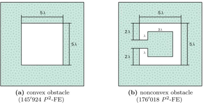
(a) convex obstacle (1451924 P2-FE) 5 2 2 5 3 (b) nonconvex obstacle (1761018 P2-FE)
Figure 4: Computational domain Ω with a convex square (a) or a nonconvex cavity (b) shaped obstacle
Usually we avoid inverting the mass-matrix at each time step via order pre-serving mass-lumping [23] which, however, introduces an additional spatial dis-cretization error. Here to ensure a consistent comparison, we thus compute uh
and u˚
hboth either with, or without, mass-lumping (ML). For the CG iteration,
245
we always choose vp0q0 ” 0, vp0q1 ” 0 and fix the tolerance to tol “ 10´14 to
ensure convergence to machine precision accuracy.
In Figure 3, we monitor the difference between the numerical solution u˚ h
or u˚
h,HDGof (4.1), obtained with a direct solver, and uh or uh,HDG, obtained
with the CMCG method using either the second or the first order formulation, 250
respectively. As expected, for increasingly smaller ∆t and a fixed stringent tolerance in the CG iteration, the numerical solution of the CMCG method always converges to the discrete solution of the Helmholtz equation for the same FE discretization.
4.2. CG iteration and initial run-up 255
Next, we first compare different stopping criteria for the CG iteration in the CMCG Algorithm applied to the original second-order formulation from Section 2. We then illustrate how the CMCG method greatly accelerates the convergence of a solution of the wave equation to its long-time asymptotic limit, in particular for nonconvex obstacles. Finally, we show how an initial run-up 260
yields a judicious initial guess for the CG iteration, which further accelerates the convergence of the CMCG Algorithm.
Hence, we consider a two-dimensional sound-soft scattering problem (2.1) with c ” 1, k “ ω “ 2π, f ” gD” gN ” 0 and gS “ ´pBn´ ikquinin a bounded
square domain Ω “ p0, 10λq ˆ p0, 10λq, λ “ 1, either with a convex obstacle or a semi-open square shaped cavity. On the boundary ΓD of the obstacle, we
impose a homogeneous Dirichlet condition and on the exterior boundary ΓS a
wave
uinpxq “ exppikpx1cospθq ` x2sinpθqqq (4.2)
impinges with the angle θ “ 135˝upon the obstacle.
4.2.1. CG iteration and stopping criteria
In Algorithm (Section 2.3), the CMCG method terminates at the `-th iter-ation and returns
up`qh “ v0p`q` pi{ωqv p`q
1 (4.3)
when the relative CG-residual in Step 5.8,
|up`qh |CG:“ g f f e }∇rp``1q0 }2L2pΩq` }p1{cq r p``1q 1 }2L2pΩq }∇r0p0q}2L2pΩq` }p1{cq r p0q 1 }2L2pΩq , (4.4)
is less than the tolerance tol. Indeed, a small CG-residual indicates that the 265
gradient of J is sufficiently small at pvp`q0 , v p`q
1 q and thus that a minimum has
been reached.
Since the cost functional J also vanishes at the minimum, we can use J itself, instead of its gradient, to monitor convergence of the CG iteration via the relative periodicity misfit,
|up`qh |J:“ b J pvp`q0 , v p`q 1 q }f }L2pΩq` }gS}L2pΓ Sq . (4.5)
In fact, the convergence criterion (4.5) is typically used in long-time simula-tions of the wave equation without controllability (“do-nothing” approach) to determine the current misfit from periodicity in the energy norm.
270
Alternatively, we may also directly compute the current relative Helmholtz residual from (2.1):
|up`qh |H:“
}Ahup`qh ´ bh}2
}bh}2
, (4.6)
where Ahand bhresult from a FE discretization of (2.1) without mass-lumping,
up`qh corresponds to the discrete vector of FE coefficients of up`qh , and }¨}2denotes
the discrete Euclidean norm.
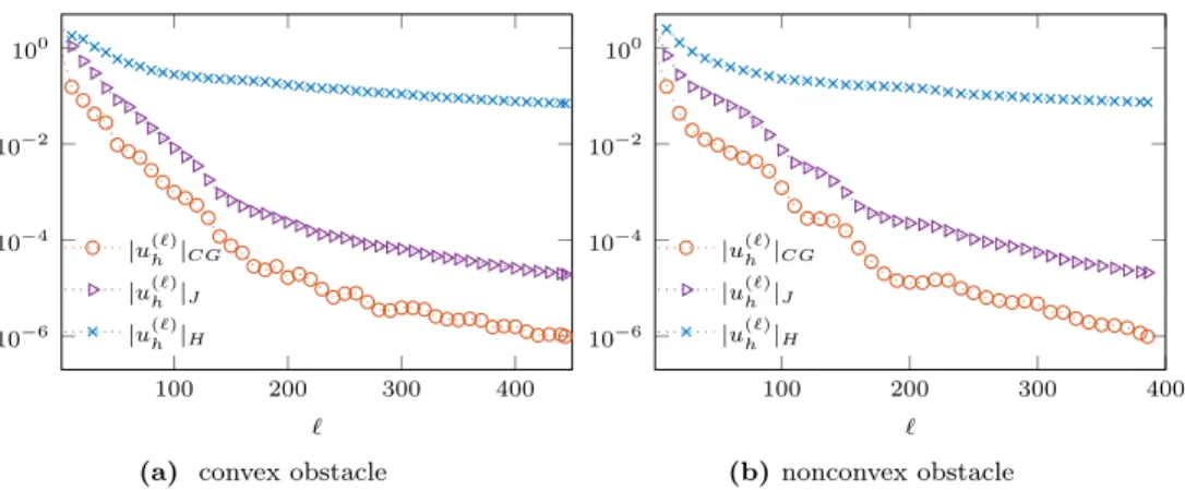
In Figure 5, we monitor |up`qh |CG, |up`qh |J and |up`qh |H, defined in (4.4)–(4.6)
for the CMCG solution up`qh at the `-th CG iteration. Whether for a convex 275
(Figure 4a) or a nonconvex (Figure 4b) obstacle, both the CG-residual |up`qh |CG
and the periodicity misfit |up`qh |J rapidly converge to zero. In contrast, the
Helmholtz residual |up`qh |H stagnates beyond the first hundred CG iterations, as
the mass-matrix that appears in Ah in (4.6) is discretized here without
mass-lumping. That additional discretization error together with the numerical error 280
in the time integration of (2.2) both prevent the discrete Helmholtz residual |up`qh |H from converging to zero; hence, (4.6) is generally not a reliable stopping
criterion for the CMCG method, unless the spatial FE discretizations used in (2.1) and (4.1) are identical.
100 200 300 400 10´6 10´4 10´2 100 ` |up`qh |CG |up`qh |J |up`qh |H
(a) convex obstacle
100 200 300 400 10´6 10´4 10´2 100 ` |up`qh |CG |up`qh |J |up`qh |H (b) nonconvex obstacle
Figure 5: CG iterations and stopping criteria: relative CG residual |up`qh |CG in (4.4),
Helmholtz residual |up`qh |H in (4.6), and periodicity mismatch |up`qh |J in (4.5) at the `-th
CG iteration.
4.2.2. CMCG method vs. long-time wave equation solver 285
In general, the solution wpx, tq of the time-harmonically forced wave equation (2.2) converges asymptotically to the time-harmonic solution [24]
wpx, tq „ Re tupxq expp´iωtqu as t Ñ `8, (4.7) where u is the (unique) solution of the Helmholtz equation (2.1). Thus, with a wave equation solver at hand, one can in principle compute u from w by solving (2.2) without controllability until a quasi-periodic regime is reached. Given the current value of wp¨, tq at time t “ ` T , ` ě 1, one can extract from it the complex-valued approximate solution of (2.1),
whp`q:“ wp¨, `T q ` i
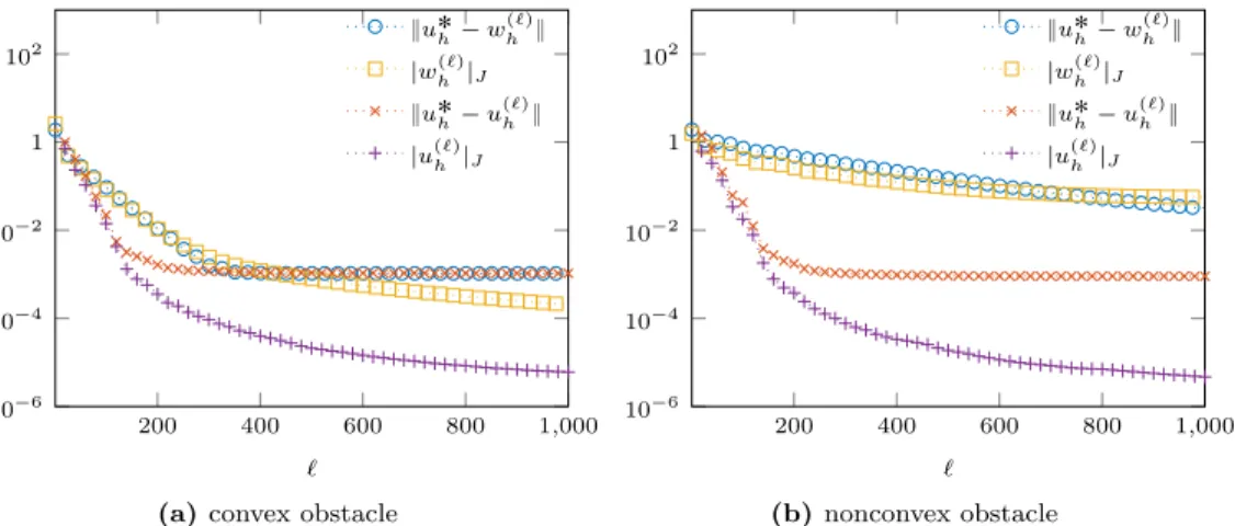
ωwtp¨, `T q, ` ě 1, T “ p2πq{ω, (4.8) which converges to u as ` Ñ `8. This “do-nothing” approach only requires the time integration of (2.2) without controllability or CG iteration, but it may converge arbitrarily slowly for nonconvex obstacles due to trapped modes [8, 11]. In Figure 6, we monitor the periodicity misfit of |up`qh |J and |wp`qh |J, where
up`qh is the CMCG solution at the `-th CG iteration and wp`qh is given by (4.8). In 290
addition, we also compare both numerical solutions with the direct solution u˚ h
of the linear system (4.1), resulting from the same underlying FE discretization, yet without mass-lumping.
We observe that the asymptotic solution whp`qand the CMCG solution up`qh in-deed both converge to the time-harmonic solution u˚
h, until the additional errors
295
caused by mass-lumping and the time discretization dominate the total error – see Section 4.1. For the convex obstacle, the number of CG iterations required by up`qh is only half the number of time periods needed for whp`qto reach the same
200 400 600 800 1,000 10´6 10´4 10´2 1 102 ` }u˚h´ whp`q} |wp`qh |J }u˚h´ up`qh } |up`qh |J
(a) convex obstacle
200 400 600 800 1,000 10´6 10´4 10´2 1 102 ` }u˚h´ whp`q} |wp`qh |J }u˚h´ up`qh } |up`qh |J (b) nonconvex obstacle Figure 6: CMCG method vs. long-time wave equation solver: plane wave scattering from a convex (a) or a nonconvex obstacle (b). Comparison between the numerical solution, up`qh , obtained with the CMCG method at the `-th CG iteration and the approximate solution wp`qh , obtained via (4.8) from the solution of the wave equation at time t “ ` T without controlla-bility.
level of accuracy. However, since each CG iteration requires not only the solu-tion of a forward and backward wave equasolu-tion but also of the elliptic problem 300
(2.16a), simply computing a long-time solution of the time-harmonically forced wave equation (2.2) without controllability in fact proves cheaper here than the CMCG Algorithm. For a nonconvex obstacle, however, the long-time numerical solution of the time-dependent wave equation wp`qh converges extremely slowly and fails to reach the asymptotic time-harmonic regime even after 1000 periods. 305
In contrast, the convergence of the CMCG solution up`qh remains remarkably insensitive to the non-convexity of the obstacle.
4.2.3. Initial run-up
In [25], Mur suggested that convergence of the time-harmonically forced wave equation (2.2) to the time-harmonic asymptotic regime can be accelerated by pre-multiplying the time-harmonic sources in (2.2) with the smooth transient function θtr from zero to one,
θtrptq “ $ & % ˆ 2 ´ sin ˆ t ttr π 2 ˙˙ sin ˆ t ttr π 2 ˙ , 0 ď t ď ttr, 1, t ě ttr, (4.9)
active during the initial time interval r0, ttrs, ttr“ ` T – see also [8].
Again, we consider plane wave scattering either from a convex or nonconvex obstacle – see Figure 4. Now, we first solve the wave equation (2.2) with the modified source terms and zero initial conditions until time t “ ` T , ` ě 1, which
0 15 30 45 60 90 120 150 300 450 600 750 888 200 400 600 800 1,000
number of time periods ` during run-up #periods in run-up
#periods in CMCG method
(a) convex obstacle
0 15 30 45 60 90 120 150 300 450 600 750 772 200 400 600 800 1,000
number of time periods ` during run-up #periods in run-up
#periods in CMCG method
(b) nonconvex obstacle
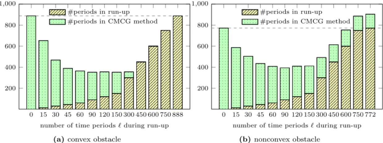
Figure 7: Initial run-up. Plane wave scattering problems from (a) a convex or (b) a non-convex obstacle: total number of forward and backward wave equations solved over one period r0, T s until convergence.
yields the time-dependent solution ytr. After that initial run-up phase, we then
apply the CMCG Algorithm (Section 2.3) using the initial guess v0p0q“ ytrp¨, `T q, v1p0q“ pytrqtp¨, `T q.
To estimate the total computational effort, we count the total number of time 310
periods for which the (forward or backward) wave equation is solved: ` during initial run-up and 2 ˆ #iterCGduring the CG iteration. In Figure 7 we display
the total number 2 ˆ #iterCG` ` of time periods needed until convergence with
tol “ 10´6, as we vary the number of periods ` in the initial run-up.
For a convex obstacle, the CMCG Algorithm without any initial run-up 315
requires 888 time periods. However, as in Section 4.2, convergence can also be achieved at a comparable computational effort simply by solving the wave equation, here with the source terms pre-multiplied by θtr in (4.9). Still, the
minimal computational cost is achieved when both the initial run-up and the CMCG Algorithm are combined.
320
For the nonconvex obstacle, however, simply solving the time-harmonically forced wave equation over a very long time, be it with or without θtrptq
smooth-ing, fails to reach the long-time asymptotic final time-harmonic state. Regard-less of the length of the initial run-up, convergence indeed cannot be achieved here (within 1000 time periods) without controllability because of trapped modes. 325
Nevertheless, the initial run-up always speeds up the convergence of the CMCG method by providing a judicious initial guess for the CG iteration.
4.3. Parallel computations
Both the CMCG method for the second-order formulation from Section 2 and that for the first-order formulation from Section 3 lead to inherently paral-330
lel non-intrusive algorithms, as long as an efficient parallel solver for the time-dependent wave equation is available. As the first-order formulation with the HDG discretization neither requires mass-lumping nor the solution of an ellip-tic problem, it is in fact trivially parallel. Here we demonstrate that even the CMCG approach for the second-order formulation, which does require the solu-335
tion of (2.16a) at each CG iteration, nonetheless achieves strong scalability on a massively parallel architecture.
The CMCG Algorithm from Section 2.3 is implemented within FreeFem++ [26], an open source finite element software written in C++. FreeFem++ defines a high-level Domain Specific Language (DSL) and natively supports distributed 340
parallelism with MPI. The parallel implementation of the CMCG method relies on the spatial decomposition of the computational domain Ω into multiple sub-domains, each assigned to a single computing core. Local finite element spaces are then defined on the local meshes of the subdomains, effectively distributing the global set of degrees of freedom across the available cores.
345
The bulk of the computational work for solving the forward and backward wave equations in Step 5.1 of the CMCG Algorithm simply consists in per-forming a sparse matrix-vector product at each time step, which is easily par-allelized in this domain decomposition framework: it amounts to performing local matrix-vector products in parallel on the local set of degrees of freedom 350
corresponding to each subdomain, followed by local exchange of shared values between neighboring subdomains.
While the explicit time integration of the wave equation is trivially paral-lelized thanks to mass-lumping, achieving good parallel scalability for the elliptic problem in Step5.2 of the CMCG Algorithm is more difficult. Here we use do-355
main decomposition (DD) methods [18], which are well-known to produce robust and scalable parallel preconditioners for the iterative solution of large scale par-tial differenpar-tial equations. We use the parallel DD library HPDDM [27], which implements efficiently various Schwarz and substructuring methods in C++11 with MPI and OpenMP for parallelism and is interfaced with FreeFem++ . 360
The elliptic problem (2.16a) in the CMCG algorithm is solved by HPDDM using a two-level overlapping Schwarz DD preconditioner, where the coarse space is built using Generalized Eigenproblems in the Overlap (GenEO) [28]. The Ge-nEO approach has proved effective in producing highly scalable preconditioners for solving various elliptic problems [6, 28].
365
All computations were performed on the supercomputer OCCIGEN at CINES, France1, with 50544 (Intel XEON Haswell ) cores.
4.3.1. 2D Marmousi Model
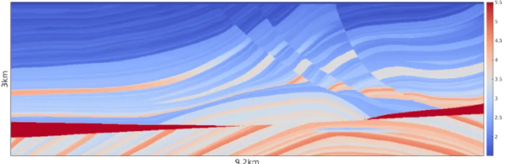
Here we consider the well-known Marmousi model from geophysics [29], that is (2.1) in Ω “ p0, 9.2q ˆ p0, 3q rkms with the source
f pxq “ expp´2000ppx ´ x˚ 1q 2 ` py ´ x˚2q 2 qq, px˚1, x˚2q “ p6, ´3{16q. 1https://www.cines.fr/calcul/materiels/occigen/
Figure 8: Marmousi model: propagation velocity 1.5 ď cpxq ď 5.5 rkm{ss
Frequency Wave number #Unknowns #Nodes ν [Hz] k “ ω{c “ 2πν{c ndof 24 cores per node 10 11 – 42 116581443 1–8 20 22 – 84 616281881 1–16 40 45 – 168 2615051761 8–64 60 68 – 252 5916301641 16–128 80 91 – 336 10610031521 16–128 160 182 – 671 42319751041 64–256 250 285 – 1048 1103512411009 128–512
Table 1: 2D-Marmousi model: P2-FE with 15 points per wave length
The velocity profile cpxq is shown in Figure 8 and we apply absorbing boundary conditions on the lateral and lower boundaries and a homogeneous Dirichlet con-dition at the top. For the spatial discretization, we use a P2-FE method with (order preserving) mass-lumping [23] and at least 15 points per wave length. For the time integration of (2.2), we apply the leap-frog scheme (LF); here, the number of T {∆t “ 390 time steps per period remains constant at all frequencies ν “ ω{2π, as both T and ∆t are inversely proportional to ν. To speed-up the convergence of the CMCG method, we also use an initial run-up (Section 4.2) until time ttr, which lets waves travel at least once across the entire
computa-tional domain during run-up; hence, we set ` “R ?9.2
2` 32
T cmin
V
, ttr “ ` T, T “ p2πq{ω.
For any particular frequency ν, we apply the CMCG method for fixed pa-rameters and FE-mesh while increasing the number of (CPU) cores. Figure 9 370
displays the real part of the wave field with ν “ 250 [Hz]. In Figure 10, we ob-serve linear speed-up (strong scaling) at every frequency with increasing number of cores. In fact, the speed-up is even slightly better than linear due to cache effects, but also because the cost of the direct solver used on each subdomain decreases superlinearly with the decreasing size of subdomains as the number 375
of cores increases.
Figure 9: 2D-Marmousi model. Real part of the wave field with ω “ 2πν, ν “ 250 [Hz] 24 48 96 192 384 768 1536 3072 6144 12288 102 103 104 1.3 10 1.2 20 1.2 40 1.1 80 1.1 160 1.1 250 cores CPU-time [sec.] ν “ 10 ν “ 20 ν “ 40 ν “ 80 ν “ 160 ν “ 250
Figure 10: 2D-Marmousi model. Total CPU-time in seconds for varying number of cores. For each frequency ν, the FE-discretization and problem size remain fixed.
decrease, so that the number of time steps per CG iteration remains constant. Since the number of CG iterations does not grow here with increasing ν, the bulk of the computational work in the CMCG Algorithm in fact shifts to the 380
run-up phase. For ν “ 10 Hz, for instance, the CMCG Algorithm stops after 273 CG iterations, while 74% of the total computational time is spent in the time integration of (2.2), 16% in the elliptic solver (DDM) and 10% in the initial run-up. In contrast, for ν “ 250 Hz, the CMCG Algorithm already stops after 5 CG iterations, while 99% of the total computational time is spent in the initial 385
run-up and 1% in the CG iteration. By modifying the run-up time ttr, one
could arbitrarily shift the relative computational cost between run-up and CG iterations and thus further optimize for a minimal total execution time. 4.3.2. 3D cavity
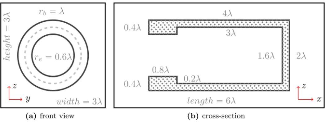
Finally, we compute the scattered wave from a sound-soft cavity – see Figure 11 – and hence consider (2.1) in Ω “ p0, 6q ˆ p0, 3q ˆ p0, 3q with c “ 1, k “ ω “
width “ 3λ heig ht “ 3 λ rb“ λ re“ 0.6λ y z
(a) front view
length “ 6λ 4λ 0.8λ 3λ 2λ 1.6λ 0.4λ 0.4λ 0.2λ x z (b) cross-section
Figure 11: 3D-cavity: a) front view of the opening with inner and outer radius, b) longitu-dinal cross-section.
Figure 12: 3D-cavity; total wave field (2.1) with c “ 1, ω “ 2πν and ν “ 6 obtained with the CMCG method
2πν, λ “ 1, f ” gD” gN ” 0 and
gS “ ´pBn´ ikquin, uinpxq “ exppik x|dq, d “ p1{2, 0,
? 3{2q|. We impose a homogeneous Dirichlet boundary condition on the obstacle and a 390
Sommerfeld-like absorbing condition on the exterior boundary of Ω.
Now, we discretize (2.2) with P1-FE in space and the second-order LF
method in time. To control the pollution error, we set hk3{2 „ const, as we
increase the frequency ν. Figure 12 shows the total wave field with ν “ 6 inside the cavity. For fixed parameters and mesh size, we now solve (2.1) at frequen-395
cies ν “ 2, 3, 4, 6 with the CMCG method using an increasing number of cores – see Table 2. Again, we observe in Figure 13 (better than) linear (strong) scaling with increasing number of cores. In contrast to the previous Marmousi problem, the ”do-nothing” approach without controllability fails here because the 3D cavity is not convex.
Frequency #Unknowns #Tetrahedra CG iterations #Nodes ν “ 2πω ndof 24 cores per node 2 8.17 ¨ 105 510511049 239 1–8
3 5.22 ¨ 106 3111901000 440 2–32
4 1.9 ¨ 107 11413911112 607 32–96
6 1.18 ¨ 108 70315901464 578 64–128
Table 2: 3D-cavity: CMCG methods with P1-FEM. As η increases, the ratio hk3{2remains
constant to avoid pollution errors [30].
24x1 24x2 24x4 24x8 24x16 24x32 24x64 24x128 102 103 104 1.2 ν “ 2 1.2 ν “ 3 1.0 ν “ 4 1.1 ν “ 6 CPU-time [sec.] ν “ 2 ν “ 3 ν “ 4 ν “ 6
Figure 13: 3D-cavity: Total CPU-time in seconds for varying number of cores. For each frequency ν, the FE-discretization and problem size remain fixed.
5. Concluding remarks
We have presented two inherently parallel controllability methods (CM) for the numerical solution of the Helmholtz equation in heterogeneous media. The first, based on the second-order formulation of the wave equation, uses a standard (continuous) FE discretization in space with order preserving mass-405
lumping. Each conjugate gradient (CG) iteration then requires the explicit time integration of a forward and backward wave equation, together with the solution of the symmetric and coercive elliptic problem (2.16), which is independent of the frequency. The second, based on the first-order (or mixed) formulation of the wave equation, uses a recent hybridized discontinuous Galerkin (HDG) dis-410
cretization, which not only automatically yields a block-diagonal mass-matrix but also completely avoids solving (2.16). Hence, it is trivially parallelized and even leads to superconvergence after a local post-processing step.
Both CMCG methods are inherently parallel, as they lead to iterative al-gorithms whose convergence rate is independent of the number of cores on a 415
distributed memory architecture. Thanks to the well-known parallel efficiency of explicit methods combined with the excellent scalability of two-level domain decomposition preconditioners for coercive elliptic problems up to thousands of cores implemented in HPDDM, even the second-order CMCG approach exhibits parallel strong scalability.
420
gov-erned by the Helmholtz equation, such as sound-soft or sound-hard scattering problems or wave propagation in physically bounded domains. Although the CMCG solution will generally contain higher order spurious eigenmodes, we have proposed in Section 2.2 a simple filtering procedure to remove them. Fur-425
thermore, including a transient initial run-up to determine a judicious initial guess significantly accelerates the CG iteration. In fact, for scattering from convex obstacles, simply solving the time-harmonically forced wave equation over a long-time without any controllability can provide an even simpler, highly parallel Helmholtz solver. For nonconvex obstacles, however, solving the wave 430
equation without any controllability (”do-nothing” approach) is not a viable option, as the long time asymptotic convergence to the time-harmonic regime is simply too slow due to trapped modes. In all cases, the CMCG Algorithm combined with the initial run-up leads to the smallest time-to-solution.
The CMCG approach developed here for the Helmholtz equation immedi-435
ately generalizes to other time-harmonic vector wave equations from electromag-netics or elasticity. Its implementation is non-intrusive and particularly useful when a parallel efficient time-dependent wave equation solver is at hand. In the presence of local mesh refinement, local time-stepping methods [31] permit to circumvent the increasingly stringent CFL condition without sacrificing the 440
explicitness or inherent parallelism. Finally, the CMCG method can also be used to compute periodic, but not necessarily time-harmonic, solutions of the wave equations. In particular, if the source consists of a superposition of several time-harmonic sources (”super-shot”) with rational frequencies, the solutions to the different Helmholtz problems can be extracted via filtering from a single 445
application of the CMCG method.
Acknowledgement: This work was supported by the Swiss National Sci-ence Foundation under grant SNF 200021 169243. Access to the HPC resources of CINES was granted under allocation 2018-A0040607330 by GENCI.
References 450
[1] O. G. Ernst, M. J. Gander, Why it is Difficult to Solve Helmholtz Prob-lems with Classical Iterative Methods, Springer Berlin Heidelberg, Berlin, Heidelberg, 2012, pp. 325–363.
[2] Y. Erlangga, C. Vuik, C. Oosterlee, On a class of preconditioners for solving the Helmholtz equation, Appl. Num. Mat. 50 (3) (2004) 409–425.
455
[3] H. Calandra, S. Gratton, X. Vasseur, A Geometric Multigrid Precondi-tioner for the Solution of the Helmholtz Equation in Three-Dimensional Heterogeneous Media on Massively Parallel Computers, Springer Internat. Publ., 2017, pp. 141–155.
[4] M. Bollh¨ofer, M. J. Grote, O. Schenk, Algebraic multilevel preconditioner 460
for the Helmholtz equation in heterogeneous media, SIAM J. Sci. Comput. 31 (5) (2009) 3781–3805.
[5] I. Graham, E. Spence, E. Vainikko, Domain decomposition preconditioning for high-frequency Helmholtz problems with absorption, Mathematics of Computation 86 (307) (2017) 2089–2127.
465
[6] M. Bonazzoli, V. Dolean, I. G. Graham, E. A. Spence, P.-H. Tournier, A two-level domain-decomposition preconditioner for the time-harmonic Maxwell’s equations, Lect. Notes Comput. Sci. Eng.
[7] B. Engquist, L. Ying, Sweeping preconditioner for the Helmholtz equation: Moving perfectly matched layers, Mult. Model. Sim. 9 (2011) 686–710. 470
[8] M.-O. Bristeau, R. Glowinski, J. P´eriaux, Controllability Methods for the Calculation of Time-Periodic Solutions. Application to Scattering, J. Com-put. Phys. 147 (2) (1998) 265–292.
[9] E. Heikkola, S. M¨onk¨ol¨a, A. Pennanen, T. Rossi, Controllability method for acoustic scattering with spectral elements, J. Comput. Appl. Math. 204 (2) 475
(2007) 344–355.
[10] E. Heikkola, S. M¨onk¨ol¨a, A. Pennanen, T. Rossi, Controllability method for the Helmholtz equation with higher-order discretizations, J. Comput. Phys. 225 (2) (2007) 1553–1576.
[11] M. J. Grote, J. H. Tang, On controllability methods for the Helmholtz 480
equation, tech. report 2018-06, University of Basel, 2018 (2018).
[12] R. Glowinski, T. Rossi, A mixed formulation and exact controllability ap-proach for the computation of the periodic solutions of the scalar wave equation.(i): Controllability problem formulation and related iterative so-lution., Comptes Rendus Math. 343 (7) (2006) 493–498.
485
[13] B. Cockburn, N. Nguyen, J. Peraire, M. Stanglmeier, An explicit hybridiz-able discontinuous Galerkin method for the acoustic wave equation, Com-put. Meth. Appl. Mech. Engrg. 300 (2016) 748–769.
[14] J.-L. Lions, Exact controllability, stabilization and perturbations for dis-tributed systems, SIAM J. Appl. Math. 30 (2) (1988) 1–68.
490
[15] A. Bayliss, M. Gunzburger, E. Turkel, Boundary conditions for the numer-ical solution of elliptic equations in exterior region, SIAM J. Appl. Math. 42 (2) (1982) 430–451.
[16] M. J. Grote, J. B. Keller, On nonreflecting boundary conditions, J. Comput. Phys. 122 (2) (1995) 231–243.
495
[17] J. M´alek, Z. Strakoˇs, Preconditioning and the Conjugate Gradient Method in the Context of Solving PDEs, SIAM, 2014.
[18] V. Dolean, P. Jolivet, F. Nataf, An Introduction to Domain Decomposition Methods. Algorithms, Theory, and Parallel Implementation, SIAM, 2015.
[19] L. C. Evans, Partial Differential Equation, AMS, 2010. 500
[20] A. Pazy, Semigroups of Linear Operators and Applications to Partial Dif-ferential Equations, Springer, 1983.
[21] P. Cummings, X. Feng, Sharp regularity coefficient estimates for complex-valued acoustic and elastic Helmholtz equations, Math. Models Methods Appl. Sci. 16 (01) (2006) 139–160.
505
[22] E. B´ecache, P. Joly, C. Tsogka, An analysis of new mixed finite elements for the approximation of wave propagation problems, SIAM J. on Numer. Anal. 37 (4) (2000) 1053–1084.
[23] G. Cohen, P. Joly, J. E. Roberts, N. Tordjman, Higher order triangular finite elements with mass lumping for the wave equation, SIAM J. Numer. 510
Anal. 38 (6) (2001) 2047–2078.
[24] C. Bardos, J. Rauch, Variational algorithms for Helmholtz equation using time evolution and artificial boundaries, Asympt. Anal. 9 (1994) 101–117. [25] G. Mur, The finite-element modeling of three-dimensional electromagnetic
fields using edge and nodal elements, IEEE Trans. on Antenn. and Prop. 515
41 (1993) 948–953.
[26] F. Hecht, New development in FreeFem++, J. Num. Math. 20 (2012) 251– 265.
[27] P. Jolivet, F. Hecht, F. Nataf, C. Prud’homme, Scalable domain decompo-sition preconditioners for heterogeneous elliptic problems, in: Proc. 2013 520
ACM/IEEE Conf. on Supercomputing, SC13, ACM, 2013, pp. 1–11. [28] N. Spillane, V. Dolean, P. Hauret, F. Nataf, C. Pechstein, R. Scheichl,
Abstract robust coarse spaces for systems of PDEs via generalized eigen-problems in the overlaps, Numer. Math. 126 (4) (2014) 741–770.
[29] A. Bourgeois, M. Bourget, P. Lailly, M. Poulet, P. Ricarte, R. Versteeg, 525
Marmousi, model and data, 1990.
[30] I. M. Babuˇska, S. A. Sauter, Is the pollution effect of the FEM avoidable for the Helmholtz equation considering high wave numbers, SIAM J. Numer. Anal. 34 (6) (1997) 2392–2423.
[31] M. J. Grote, D. Peter, M. Rietmann, O. Schenk, Newmark local time step-530
ping on high-performance computing architectures, J. Comput. Phys. 334 (2017) 308–326.
![Figure 9: 2D-Marmousi model. Real part of the wave field with ω “ 2πν, ν “ 250 [Hz] 24 48 96 192 384 768 1536 3072 6144 122881021031041.3101.2201.2401.1801.11601.1 250 coresCPU-time[sec.] ν “ 10ν“20ν“40ν“80ν“ 160ν“250](https://thumb-eu.123doks.com/thumbv2/123doknet/15005807.676867/25.918.206.713.186.419/figure-marmousi-model-real-wave-field-πν-corescpu.webp)