HAL Id: cea-02183138
https://hal-cea.archives-ouvertes.fr/cea-02183138
Submitted on 15 Jul 2019HAL is a multi-disciplinary open access archive for the deposit and dissemination of sci-entific research documents, whether they are pub-lished or not. The documents may come from teaching and research institutions in France or abroad, or from public or private research centers.
L’archive ouverte pluridisciplinaire HAL, est destinée au dépôt et à la diffusion de documents scientifiques de niveau recherche, publiés ou non, émanant des établissements d’enseignement et de recherche français ou étrangers, des laboratoires publics ou privés.
the 4th dimension in grand-canonical simulation
Luc Belloni
To cite this version:
Luc Belloni. Non-equilibrium hybrid insertion/extraction through the 4th dimension in grand-canonical simulation. Journal of Chemical Physics, American Institute of Physics, 2019, 151 (2), pp.021101. �10.1063/1.5110478�. �cea-02183138�
Non-equilibrium Hybrid Insertion/Extraction through the 4th Dimension in
Grand-Canonical Simulation
Luc Belloni
LIONS, NIMBE, CEA, CNRS, Université Paris-Saclay, 91191-Gif-sur-Yvette, France
Abstract:
The process of inserting/deleting a particle during Grand-Canonical Monte-Carlo (MC) simulations is investigated using a novel, original technique: the trial event is made of a short non-equilibrium molecular dynamics (MD) trajectory during which a coordinate w along a 4th dimension is added to the particle in course of insertion/deletion and is forced to decrease from large values up to zero (for insertion) or increased from 0 up to large values (for extraction) at imposed vw velocity. The probability of acceptation of the whole MC move is
controlled by the chemical potential and the external work applied during the trajectory. Contrary to the standard procedures which create/delete suddenly a particle, the proposed technique gives time to the fluid environment to relax during the gradual insertion/extraction before acceptation decision. The reward for this expensive trial move is a gain of many orders of magnitude in success rate. The power and wide domain of interest of this hybrid "H4D" algorithm which marries stochastic MC and non-equilibrium deterministic MD flavors are briefly illustrated with hard sphere, water and electrolyte systems. The same approach can be easily adapted in order to measure the chemical potential of a solute particle immersed in a fluid during canonical or isobaric simulations. It then becomes an efficient application of the Jarzynski theorem for the determination of solvation free energy.
Introduction
Within numerical simulations, the ability to measure or to impose the chemical potential (CP) provides valuable extra information. In the first case, the simulation is performed in NVT canonical or NPT isobaric conditions (N is the number of particles, V the volume, T the temperature and P the pressure) and the objective is the CP of an extra, solute particle. This may be a particle of the fluid itself when one wants to complete its equation of
state (T,) or (T,P) (=N/V is the number density) or is really a unique
molecular/macromolecular solute immersed at infinite dilution in the bulk solvent in order to determine its excess CP exc or solvation free energy. The fundamental Widom's insertion
technique 1 creates suddenly a solute particle at random position inside a bulk solvent cell,
calculates its experienced interaction potential vsolute and averages the Boltzmann factor
ln vsolute
exc
solvent
e
(=1/kT is the inverse thermal energy). The inverse version starts
from a solvent+solute simulation cell and follows the difference of energy induced by the
sudden deletion of the solute, exc ln vsolute
solvent solute
e
. While formally exact, both
techniques become rapidly inefficient in dense, cohesive systems where the interesting configurations which contribute the most to the averages are rarely if not never sampled. The Bennett's overlapping distribution technique 2 3 which couples information from both simulations improves the precision but is still insufficient for multi-site solute molecules. So, a wide spectrum of theoretical approaches has been elaborated in the literature in order to circumvent this difficulty and calculate chemical potentials or free energy differences with great precision. They all share the use of "partial" solutes which interact with the solvent particles through a pair potential v that interpolates continuously between v=0=0 (no solute) and v=1=v (full solute, real potential v). Among the possible approaches 4, one briefly cites the
thermodynamical integration and the free energy perturbation which require performing in parallel 20-40 simulations, each at a different intermediate fixed state . Other techniques treat as an extra degree of freedom, subject to a prescribed dynamics, and construct the potential of mean-force from the measured -distribution 5 6. Finally, the Jarzynski's approach 7 imposes a time-dependent law (t) during a non-equilibrium simulation joining the two
opposite states =0 and 1, and construct the CP from the external work W exerted on the solvent+partial solute system, exc ln eW .
In the second case, the simulation is performed in VT Grand-Canonical (GC) ensemble which imposes the value of the solvent CP through exchanges of particles with a reservoir. This type of simulation is needed in heterogeneous interfacial or porous media in equilibrium with a bulk solvent. In homogeneous systems, it provides direct access to fundamental thermodynamical quantities from the particle number fluctuations <N2> around the mean
value <N>. The repeated trial addition/subtraction of particles along the simulation suffers from the same difficulties as above: a trial random instantaneous insertion in a cell containing N particles will mainly conduct to an overlap and miss the interesting N+1 configurations, leading to a sure rejection. Inversely, a randomly chosen particle in the cell experiences a favorable (highly negative) energy inside its environment, not compatible with its sudden
deletion. The probability of acceptation is for instance 10-7 for a hard sphere fluid just below
crystallization and less than 10-4 for a bulk water system. Admittedly, cavity-bias 8 and orientational-bias 4 techniques optimize the search for the very rare interesting locations for insertion or the very rare unhappy molecules for deletion and provide a reasonable increase in effective acceptation rate, but with known side-effects when the fluid has no time to relax between successive N±1 events 9. The direct use of "partial" particles as above, with stochastic
or deterministic trajectory 10 during the simulation, is not satisfactory here except if one accepts to explore the phase space with a non-integer, continuous N number in the cell.
Grand Canonical H4D algorithm
In the present work, we propose a different, new strategy for changing the particle number N. For a simple introduction, we ask the reader to think about the way a triangular rack is progressively filled with balls at the beginning of a billiards game: the balls can be considered as 2D disks which collide inside the horizontal, partially filled cell. How to add an extra ball? A standard naïve "GC" procedure would freeze a configuration and try to create suddenly a new disk at a 2D position on the plane, chosen randomly or in a biased fashion. The success would be obviously rather poor. On the other hand, the clear procedure in real life restores the 3D character of the balls, the extra one is pushed down from above the table while the horizontal fluid is still moving and the collisions in 3D space between all N+1 spheres guarantees the on-the-fly creation of a 2D cavity and relaxation of the fluid. With this simple picture in mind, we now return to the 3D GC numerical simulations: a coordinate w (say, w≥0) along a 4th dimension 11 6, let us still call it the altitude, is added to the "flying" particle in course of insertion/deletion. A trial Monte-Carlo (MC) N change is made of a short Molecular Dynamics (MD) trajectory of the whole fluid performed under non-equilibrium conditions characterized by a time-dependent w(t) imposed descent/ascent law. The external work needed to maintain this law from w=+∞/0 up to w=0/+∞ is combined with the imposed CP and monitors the probability of acceptation according to the GC MC recipe. Note that the use of a "partial" particle characterized by finite w which interpolates continuously between ideal and full coupling is here only transitory and limited to the trial MC event. Such type of "hybrid" 12, non-equilibrium MC-MD combination has already been used in the literature in order to favor giant steps and overcome energy barriers in canonical simulations 13 14 15. We call our present strategy for GC particle exchanges "Hybrid 4 Dimension" or H4D.
The details of the procedure are the following.
The 3D fluid molecules interact via site-site spherically symmetric pair potentials of the form vij(rij) where rij ri rj is the ij separation. The configuration space is explored with standard
MC translations/rotations. During a particle exchange with the reservoir, the interaction
potentials become
2 2
( )
ij ij i j
v r w w where the altitude wi remains 0 for a site of the fluid
and is w for a site of the flying particle at the altitude w. At the beginning of a trial insertion, the "old" configuration contains N particles with the total potential energy Uo. The GC weight
of the configuration is 1 ! o U N o p e e N
. An extra particle is put at a random 3D
wmax is common to all sites. In case of flexible molecules, the intra configuration is drawn
from the distribution in vacuum. wmax is the first of a long list of free parameters which can be
chosen at will in order to optimize the efficiency of the technique. wmax=0 corresponds to the
usual procedure with instantaneous creation. Too short values, say less than the site diameters, would provoke probable overlaps since the beginning. Too large values are unnecessary and would require very long MD trajectories. At time t=0, the N+1 3D old velocities old
i
v are drawn from the probability density pinsertion( )v (free). In all cases, we have chosen the natural i Maxwell-Boltzmann distribution 2 ( ) exp 2 i insertion i mv p v kT
where m is the mass. In kT m /
units used in the following, the 3D velocities are of the order one. For rigid molecules, the angular velocities are drawn from similar distribution involving the inertia moments. Then, the 3D trajectory followed by the N+1 particles is provided by a non-equilibrium MD simulation during which the altitude w decreases with an imposed, constant –vw descent
velocity (vw>0, free). Again, vw=∞ corresponds to the standard creation process. The opposite
limit vw→0 would characterize a quasi-static insertion. For hard systems, the trajectory is
made of successive elastic collisions in 4D space. For continuous potentials, the equations of motion are integrated with a finite time step t (free) and a time-reversible, area-preserving algorithm 16. The N fluid particles are forced to stay always on the "horizontal" 3D space, w=0, thank to external "vertical" forces which do not produce work. The force field which controls the MD trajectory may derive from a simplified, degraded version (free) of the original potentials vij(r) in order to speed up the calculations, like using shorter cut-offs in
Ewald summations, at the risk of producing a final configuration not favorable for the true interaction. Once the flying particle has landed on the ground at w=0, the MD stops and the trial "new" (N+1) configuration is characterized by the velocities new
i
v , the total potential
energy Un and weight ( 1)
1 ( 1)! n U N n p e e N
. Inversely, a trial extraction from an old
configuration starts by choosing randomly the future flying particle among the N fluid ones. The N 3D velocities are drawn from a probability density pdestruction( )v (free), again i exclusively chosen here as the Maxwell-Boltzmann law. The non-equilibrium MD starts
while the flying particle takes off from w=0 with the very same constant ascent velocity +vw
and finishes when w reaches wmax, where the flying particle is finally entirely decoupled from
the remaining N-1 fluid particles (w=∞). The MD algorithm and the time step t are identical to those in the insertion process.
We are now ready to express the probability of acceptation of the trial particle exchange. The transition matrix from the old to the new configuration (o→n) depends only on the choice of the initial velocities since the MD is a deterministic process (and the algorithm conserves phase space volumes):
1/ / 1 ( ) ( ) o N N K old ins des i i o n p v e
(1)where Ko is the kinetic energy of the old configuration. Since the MD algorithm is
time-reversible (in fact, one just requires that the two algorithms used during insertion and destruction for integrating the equations of motion are time-inverses one to each other), the inverse transition matrix which produces the old configuration from the new one reads:
1/ / 1 ( ) ( ) n N N K new des ins i i n o p v e
(2)where Kn is the kinetic energy of the new configuration. According to the detailed balance
condition 4, the Metropolis probability of acceptation of the trial particle exchange becomes finally: ( ) ( ) min 1, ( ) min 1, insertion 1 min 1, destruction on on n o H H p n o acc o n o n p aV e N N e aV (3)
where a=e represents the activity and Hon=Hn-Ho is the change of the total mechanical
energy H=K+U from the old to the new configuration. In the present adiabatic H4D version
where the trial non-equilibrium MD trajectory is produced without thermostat, there is no
exchange of heat with the exterior and the change of total energy is equal to the external work W required to maintain fixed the vertical velocity vw despite the numerous 4D collisions with
the bulk. For continuous potentials, the equations of motion are not integrated exactly due to the finite t step and the strict equality Hon=W does not hold. Nevertheless, the MC rule (3)
always applies 17. The only risk of choosing a too large t value in order to shorten the MD
simulation is to produce too wild positive departures of Hon and to automatically reduce the
acceptation rate.
Compared to the standard procedure (wmax=0 or vw=∞, Hon=Uon), the described H4D new
technique replaces a very cheap trial exchange (cost=1 particle energy evaluation) by a very expensive one (cost=wmax/(vwt) MD time steps for N particles). The reward is that the bulk
environment has time to react to the smooth insertion/extraction process before acceptation decision and the success rate increases by orders of magnitude. Moreover, when the particle exchange has been accepted, the produced configuration is characteristic of the new N value (and does not belong to the far positive aisle of the energy spectrum as with the usual techniques) and the MD trajectory has not been waste of time because it has enabled to shuffle the whole cell. Three preliminary examples of application are briefly presented now. Technical details are given in the Supplementary Material (SM).
Hard-sphere fluid
For pure hard sphere systems (diameter=), the acceptation rate within the standard procedure is easily estimated from the last line of (3) and roughly equals the inverse activity
coefficient 1/=/a= e-exc. This explains why the GC equations of state () reported in the
literature are limited to *=3≈0.7-0.8 (≈103-104) 18 19, well below the fluid-crystal phase transition which appears at F*=0.94, ≈107 4. On the other hand, the present H4D technique
enables to cover the whole fluid range and even a large part of the metastable fluid branch
beyond F*, up to *≈1 (53% volume fraction), see Figure 1. While the probability of
acceptation of the standard technique falls off more than exponentially from 10-2 to 10-9 when
* goes from 0.6 to 1, it only slightly decreases from 55% to 15% with the H4D parameters
wmax=, vw≈0.1. An overlap is (almost) always experienced during insertion in the former
case, while it never happens in the latter case. It is interesting to note that when approaches F*, the hard sphere system spontaneously switches between two "phases" of different
densities, one fluid, the other crystallized! Above F*, the crystal eventually wins.
Figure 1: Chemical potential versus density * for the hard sphere system. The symbols refer to the present H4D technique (wmax=, vw=0.1) used in GC (diamonds) or
canonical (triangles) conditions. The cell size is L=5 for *<0.9 (N≈100) and L≈6.3 for *>0.9 (N≈235). Dotted line: analytical equation of state of Hall 20.
Liquid water
The chemical potential of the popular SPC/E water model at room conditions has been recently measured with great precision using canonical, isobaric and standard GC Monte-Carlo simulations: =-15.37kT (where the activity a is expressed in Å-3) 21. We have repeated
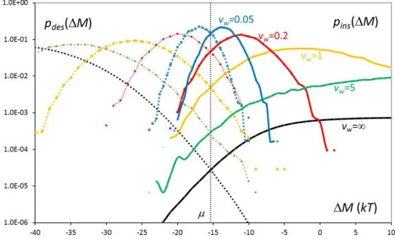
the GC simulation, this time using the H4D technique, see SM. Figure 2 presents the distributions pins(M) and pdes(M) of generalized energy change M observed during the
trial particle exchanges, where M H kTlnN 1
V
for insertion and
lnV
M H kT
N
According to the Crooks theorem 22 (the non-equilibrium version of the Bennett's 2), the two
distributions verify:
( ) ( ) M
des ins
p M ep M e (4)
and, in particular, cross at M=. While the standard technique experiences very different energy transfers in the two directions (mainly excluded volume overlaps at insertion, highly negative cohesive energy at destruction), the two H4D distributions explore narrower, overlapped energy domains and take much higher values at the crossing point, see figure 2. As a consequence, the acceptation rate increases from 9 10-5 at vw=∞ up to 0.38 at vw=0.05.
An optimal compromise between N exchange success and speed of calculation is obtained with vw≈0.2 (14% success rate).
Figure 2: Distributions of generalized energy change M observed during insertion (solid lines, right) and destruction (dotted lines, left) in GC simulation of SPC/E water system. Each curve is colored and labelled with the value of the vertical velocity vw used in H4D procedure
(vw=∞ corresponds to the usual technique). All insertion/destruction pairs cross at
M==-15.37kT.
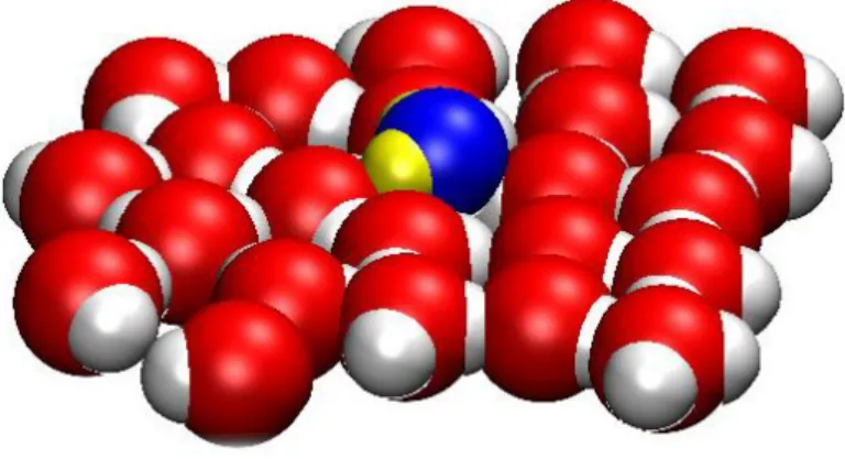
As an illuminating illustration, a video movie shows the MC/H4D procedure working for the insertion of a H2O molecule into a 2D water layer using the 3rd dimension. Figure 3
Figure 3: MC/H4D insertion of a H2O molecule into a 2D water layer through the 3rd
dimension. Snapshot taken at w=1Å. The video movie illustrates the on-the-fly reorganization of the H-bonding network in order to accommodate the extra molecule. A destruction event with gradual filling of the growing cavity left by the leaving particle simply corresponds to
the inverse movie (Multimedia view).
NaCl electrolyte
Lastly, we show how the H4D technique can be generalized for a Monte-Carlo simulation of NaCl aqueous electrolyte at the molecular solvent level of description, in the ensemble NsolventsaltPT. The number of SPC/E H2O molecules is fixed, the volume fluctuates
at the imposed pressure P=1bar and the number of ion pairs NNa+=NCl-=Nsalt varies through
exchanges with a salt reservoir which imposes the chemical potential salt=Na++Cl-. To the
author's knowledge, this is the very first time that a simulation investigates such type of
ensembles with trial ion transfers in bulk water. The electrostatic coupling is strong,
especially inside the solvation layers. Moreover, the process must involve the simultaneous insertion or destruction of two ions, one cation, one anion in order to preserve the electroneutrality. As a consequence, the trial transfer needs to operate very slowly, with a small vertical velocity, in order to reach reasonable acceptation rates, in the 1% range, and the
computational cost is heavy. Nevertheless, the simulation of a 1M NaCl aqueous solution at
room conditions has been successfully realized. The salt chemical potential has been first estimated from measurements during isobaric simulations (see below), salt=-301.1kT. Then,
the H4D-GCMC simulation has been performed with NH2O=550 solvent molecules, wmax=3Å,
vw=0.0125 and special tricks, see SM for the details. The resulting ion number fluctuates
around the average <Nsalt>≈10.2 with a root mean square fluctuation Nsalt2 ≈2.2. The mean densities are <salt>=1.01M, <H2O>=54.4M. The combination of volume + ion number
exchanges in this two-component mixture is sufficient to account for total density as well as composition fluctuations, so for all cross partial density fluctuations, and the full Kirkwood-Buff theory applies 23. For instance, the osmotic compressibility is given by:
h o2 2 salt salt osmotic osmotic T, salt V P (5)
and equals osmotic≈0.45±0.03 in the present 1M solution. At the same time, the radial pair
distribution functions gij(r) are not affected by the so-called explicit finite-size corrections so
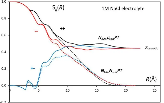
disturbing in the usual canonical or isobaric simulations of mixtures 24 25, which result from the absence of fluctuations and prevent the direct determination of the Kirkwood-Buff integrals and thermodynamic derivatives. As an illustration, figure 4 plots the 3 "running" ion-ion structure factors
0
( ) R( ( ) 1)
ij ij salt ij
S R
g r dr . They all converge to the commonasymptote osmotic (the same value as above) in the present ensemble while they are useless (without special corrections) in the NiPT ensemble.
Figure 4: Running ion-ion structure factors Sij(R) in 1M NaCl electrolyte.MC simulation with
NH2O=550. Dashed lines: the number of ions is fixed, Nsalt=10; Solid lines: Nsalt fluctuates
through H4D exchanges with a salt reservoir, salt=-301.1.
Canonical or isobaric H4D version
Up to now, the H4D technique has been described as a Grand-Canonical strategy for performing addition/subtraction of bulk fluid particles. It can be used as well for measuring the chemical potential or solvation free energy of a solute particle during canonical or isobaric simulations. The starting point considers the average of the Markov flux ratio:
( ) ( ) ( ) ( ) ( ) ( ) 1 n n o o n o o o n n n o n p p n o n o p o n o n p o n p p n o p
(6)From (3)(6), the CP of the fluid is thus given by:
ln ln insertion 1 ln ln destruction on on H M ins ins H M des des V e e N N e e V (7)
These expressions, originally established in GC ensemble, can be used as well in canonical or isobaric conditions for N fixed to the averaged GC value (with the undesired presence of finite-size perturbations in the former case). For the hard sphere system, H4D-NVT data added in figure 1 nicely agree with the GC curve on the whole fluid branch.
Moreover, the same reasoning can be followed for a solvent+solute mixture at infinite dilution of the solute and the final expression for the solvation free energy of the solute reads:
exc solute puresolvent solvent+solute ln insertion ln destruction M M e e (8)
where M=Hon for a H4D insertion of a solute inside a bulk solvent cell and M=-Hon for a
H4D extraction of the solute from a solvent+solute cell. This is nothing but an application of the Jarzynski's theorem. As usual, the combination of the insertion and destruction M distribution data with the help of the Crooks theorem (4) and well-developed BAR techniques provide better statistic precision.
Conclusion
In this letter, we have introduced the bare version of the new H4D technique for efficient Grand-Canonical insertions/extractions which enables to treat otherwise unreachable new systems. The very same procedure helps in measuring the solvation free energy of solute molecules. The detailed application on various solvents, mixtures, solutes and the developments of more complex and optimized versions will be described in future papers.
Supplementary material: See supplementary material for the technical details in the hard-sphere, water and electrolyte applications of the H4D algorithm.
Acknowledgment: The author would thank A. Thill, D. Borgis and M. Levesque for fruitful discussions during the tortuous elaboration of the technique.
References
1. B. Widom, J. Chem. Phys. 39, 2808 (1963) 2. C. H. Bennett, J. Comput. Phys. 22, 245 (1976)
3. K. S. Shing and K. E. Gubbins, Mol. Phys. 49, 1121 (1983)
4. D. Frenkel and B. Smit. Understanding Molecular Simulation; Academic Press, 1996. 5. X. Kong and I. C.L. Brooks, J. Chem. Phys. 105, 2414 (1996)
6. R. Pomès, E. Eisenmesser, C. B. Post, and B. Roux, J. Chem. Phys. 111, 3387 (1999) 7. C. Jarzynski, Phys. Rev. Lett. 78, 2690 (1997)
8. M. Mezei, Mol. Phys. 40, 901 (1980)
9. J. C. Shelley and G. N. Patey, J. Chem. Phys. 102, 7656 (1995) 10. T. Cagin and B. M. Pettitt, Mol. Phys. 72, 169 (1991)
11. T. C. Beutler and W. F. van Gunsteren, J. Chem. Phys. 101, 1417 (1994) 12. B. Mehling, D. W. Heermann, and B. M. Forrest, Phys. Rev. B 45, 679 (1992) 13. H. A. Stern, J. Chem. Phys. 126, 164112 (2007)
14. A. J. Ballard and C. Jarzynski, Proc. Natl. Acad. Sci.(USA) 106, 12224 (2009) 15. Y. Chen and B. Roux, J. Chem. Phys. 141, 114107 (2014)
16. N. Matubayasi and M. Nakahara, J. Chem. Phys. 110, 3291 (1999) 17. Y. Chen and B. Roux, J. Chem. Phys. 142, 024101 (2015)
18. D. J. Adams, Mol. Phys. 28, 1241 (1974)
19. B.. F.D. Smit, J. Phys.: Condens. Matter 1, 8659 (1989) 20. K. R. Hall, J. Chem. Phys. 57, 2252 (1972)
21. L. Belloni, J. Chem. Phys. 149, 094111 (2018) 22. G. E. Crooks, Phys. Rev. E 60, 2721 (1999)
24. A. Perera, L. Zoranic, S. Sokolic, and R. Mazighi, J. Mol. Liq. 159, 52 (2011)
25. P. Krüger, S. K. Schnell, D. Bedeaux, S. Kjelstrup, T. J.H. Vlugt, and J. Simon, J. Phys. Chem. Lett. 4, 235 (2013)