Three-dimensional climatological distribution of tropospheric OH' Update and evaluation

HAL Id: hal-02864989

https://hal.archives-ouvertes.fr/hal-02864989

Submitted on 11 Jun 2020

HAL is a multi-disciplinary open access

archive for the deposit and dissemination of

sci-entific research documents, whether they are

pub-lished or not. The documents may come from

teaching and research institutions in France or

abroad, or from public or private research centers.

L’archive ouverte pluridisciplinaire HAL, est

destinée au dépôt et à la diffusion de documents

scientifiques de niveau recherche, publiés ou non,

émanant des établissements d’enseignement et de

recherche français ou étrangers, des laboratoires

publics ou privés.

Three-dimensional climatological distribution of

tropospheric OH’ Update and evaluation

C. M. Spivakovsk, J. A. Logan, S. A. Montzka, Yves Balkanski, M.

Foreman-Fowler, D . B. A. Jones, L. W. Horowitz, a C Fusco, C. A. M.

Brenninkmeijer, M. J. Prather, et al.

To cite this version:

C. M. Spivakovsk, J. A. Logan, S. A. Montzka, Yves Balkanski, M. Foreman-Fowler, et al..

Three-dimensional climatological distribution of tropospheric OH’ Update and evaluation. Journal of

Geo-physical Research: Atmospheres, American GeoGeo-physical Union, 2000, 105, �10.1029/1999JD901006�.

�hal-02864989�

JOURNAL OF GEOPHYSICAL RESEARCH, VOL. 105, NO. D7, PAGES 8931-8980, APRIL 16, 2000

Three-dimensional climatological distribution of

tropospheric OH' Update and evaluation

C. M. Spivakovsky,

1 J. A. Logan,

1 S. A. Montzka,

2 Y. J. Balkanski,

1'3

M. Foreman-Fowler,

TM

D. B. A. Jones,

1 L. W. Horowitz

1,• A C Fusco,

1

C. A.M. Brenninkmeijer,

e M. J. Prather,

7 S.C. Wofsy,

• and M. B. McElroy

•

Abstract.

A global climatological distribution of tropospheric OH is com-

puted using observed

distributions

of 03, H20, NOt (NO2+NO+2N2Os+NO3

+HNO2+HNO4), CO, hydrocarbons,

temperature, and cloud optical depth. Globa.1

annual

mean

OH is 1.16 x 10

• molecules

crn

-3 (integrated

with respect

to mass

of

air up to 100 hPa within 4-32

ø latitude and up to 200 hPa outside that region).

Mean hemispheric

concentrations

of OH are nearly equal. While global mean OH

increased

by 33% compared

to that from Spivakovsky

et al. [1990], mean loss

frequencies of CH3CCi3 and CH4 increased by only 23% because a lower fraction of total OH resides in the lower troposphere in the present distribution. The value for

temperature

used for determining

lifetimes of hydrochlorofiuorocarbons

(HCFCs)

by scaling

r•te constants

[Prather and Spivakovsky,

1990] is revised

from 277 K to

272 K. The present distribution of OH is consistent within a few percent with the

current budgets of CH3CC13 and HCFC-22. For CH3CC13, it results in a lifetime

of 4.6 years, including stratospheric and ocean sinks with atmospheric lifetimes of

43 and 80 years, respectively. For HCFC-22, the lifetime is 11.4 years, allowing

for the stratospheric sink with an atmospheric lifetime of 229 years. Corrections

suggested

by observed

levels of CH2C12 (•nnu•l means) depend strongly on the

rate of interhemispheric mixing in the model. An increase in OH in the Northern

Hemisphere

by 20% combined

with a decrease

in the southern tropics by 25% is

suggested if this rate is at its upper limit consistent with observations of CFCs

•nd SSKr. For the lower

limit, observations

of CH2C12

imply •n increase

in OH in

the Northern

Hemisphere

by 35% combi'ned

with a decrease

in OH in the southern

tropics by 60%. However, such large corrections

are inconsistent

with observations

for 14CO

in the tropics

and for the interhemispheric

gradient

of CH3CC13.

Industrial

sources

of CH2C12 are sufficient for balancing its budget. The available tests do

not establish significant errors in OH except for a possible underestimate in winter

in the northern and southern tropics by 15-20% and 10-15%, respectively,

and an

overestimate in southern extratropics by ,-•25%. Observations of seasonal variations

of CH3CC13,

CH2C12,

14CO,

and C2H6 offer no evidence

for higher

levels

of OH in

the southern than in the northern extratropics. It is expected that in the next few

years the latitudinal distribution and •nnu•l cycle of CH3CC13 will be determined primarily by its loss frequency, allowing for additional constraints for OH on scales smaller than global.

1. Introduction

Ever since Levy [1971] presented a model of tropo-

spheric chemistry with the hydroxyl radical as the key species, efforts have continued to estimate accurately

its concentration in the troposphere [e.g., McConnell

et al., 1971; Weinstock and Niki, 1972; Warneck, 1974; Wofsy, 1976; Singh, 1977a, b; Lovelock, 1977; Crutzen and Fishman, 1977; Fishman et al., 1979; Makide and

Copyright 2000 by the American Geophysical Union. Paper number 1999JD901006.

0148-0227/00/1999JD901006509.00

•Department of Earth and Planetary Sciences and Divi-

sion of Engineering and Applied Sciences, Harvard Univer- sity, Cambridge, Massachusetts.

2NOAA Climate Monitoring and Diagnostics Laboratory,

Boulder, Colorado.

3Now at Laboratoire des Sciences du Climat et de l'Envi-

ronnement, Gif-sur Yvette, France.

4Now at Steelhead Machine and Design Company, Albu-

querque, New Mexico.

SNow at A•mospheric and Oceanic Sciences Program,

Princeton University, Princeton, New Jersey.

6Max Planck Institute for Chemistry, Mainz, Germany. 7Department of Geoscience, University of California, Ir-

vine. 8931

8932 SPIVAKOVSKY ET AL.: CLIMATOLOGICAL DISTRIBUTION OF TROPOSPHERIC OH

Rowland, 1981; Logan et al., 1981; Chameides and Tan,

1981; Volz et al., 1981; Crutzen and Gidel, 1983; Prinn et al., 1983, 1987, 1992, 1995; I(halil and Rasmussen, 1984; Fraser et al., 1986; Thompson and Cicerone, 1986a, b; $pivakovsky et al., 1990; Thompson et al., 1990; Crutzen and Zimmermann, 1991; Brenninkmei- jet et al., 1992; Maket al., 1992, 1994; Krol et al.

1998]. The abundance of OH determines lifetimes for

CH4, CO, and a variety of industrial pollutants, but the quest for accuracy has roots beyond the need to esti- mate the lifetimes of these gases. The chemistry of OH

comprises tightly coupled, mutually compensating re-

actions which in effect provide a buffer against changes in precursors and rate constants. Decades apart, Levg

[1971], Logan et al. [1981], and Spivakovskg et al. [1990]

derived similar estimates for the abundance of OH in

the troposphere despite considerable evolution in the understanding of both the chemical mechanism and the

characterization of precursors. Errors of 15-25% in the

global mean concentration of OH may signify major misconceptions about the chemistry or the abundance

of precursors of OH in the troposphere. At the same

time, testing global models for OH has been associated with uncertainties of a similar or larger magnitude in- trinsic to deriving an estimate indirectly from budgets

of species for which reaction with OH provides the dom-

inant sink and the sources are believed to be known:

CHaCCla [e.g., $ingh, 1977a, b; Lovelock, 1977; Makide

and Rowland, 1981; Logan et al., 1981; Chameides and Tan, 1981; I•'halil and Rasmussen, 1984; Fraser et al.,

1986; Prinn et al., 1983, 1987, 1992, 1995] and •4CO

[e.g., Weinstock and Niki, 1972; Volz et al., 1981; Bren-

ninkmeijer et al., 1992; Mak et al., 1992, 1994] (see Thompson [1994] for a review of studies of tropospheric OH through the early 1990s).

Significant recent developments have affected both di-

rect and indirect methods for estimating the abundance of OH in the troposphere. Most notably, the budget of

CHaCCla was modified by an 18% decrease in the cal-

ibration of CHaCCla [Prinn et al., 1995], a decrease in

the recommended rate constant for reaction with OH

(by ,•15% at 277 K) [Talukdar et al., 1992] and the discovery of an ocean sink [Butler et al., 1991]. Obser- vations of Brenninkmeijer et al. [1992], Brenninkmeijer [1993] and Mak et al. [1992, 1994], together with ear- lier measurements of Volz et al. [1981], provided for

the first time a comprehensive description of the tro-

pospheric distribution of •4CO. Initial interpretation of

these measurements indicated significantly higher con-

centrations of OH than those predicted by models or

inferred from the budget of CHaCCla at the time [Mak et al., 1992]. In addition, lower concentrations of

in the Southern

Hemisphere

(SH) than in the North-

ern Hemisphere (NH) led to the suggestion that con-

centrations of OH are significantly lower in northern

than in southern

midlatitudes

[Brenninkmeijer

et al.,

1992],

whereas

most models

predicted

slightly

higher

concentrations of OH in the north [e.g., $pivakovskg et

al., 1990, Crutzen and Zimmermann, 1991]. Increas-

ingly, however, it has been recognized that concentra-

tions of •4CO are as sensitive to rates of transport in

the atmosphere as to the abundance of OH and that

the initial interpretations of observations of •4CO must be revised [$pivakovskg and Balkanski, 1994; Maket al., 1994; Brenninkmeijer et al., 1999; P. Quay

(Atmospheric

•4CO: A tracer of OH concentration

and

mixing rates, submitted to Journal of Geophgsical Re-

search, 1999)].

Recent developments affecting the computation of

tropospheric OH include the suggestion by Michelsen et

al. [1994]

of a nonnegligible

quantum

yield for O(•D)

at wavelengths between 312 to 320 nm, confirmed by

laboratory measurements [Talukdar et al., 1998]. There

have been changes in recommendations for other key

rate constants [DeMote et al., 1994, 1997], in particular,

a decrease in the rate for reaction of OH with methane

(19% at 277 K). New observational data afford a bet-

ter definition of precursors for OH, such as 03, NOt

(defined as NO2 + NO + 2N205 +NOa + HNO2 + HNO4), CO, and H20. Reactions with nonmethane hy- drocarbons (NMHC), omitted in earlier studies because

of lack of observations, can now be included. The distri-

bution of cloud cover, highly uncertain in the past, can

now be constrained by a global climatology afforded by

satellite observations, International Satellite Cloud Cli- matology Project (ISCCP) [Rossow and $chiffer, 1991].

Remarkable advances have been made in measuring

concentrations of OH [e.g., Eisele et al., 1997; Mount et

al., 1997; Tanner et al., 19971; Mather et al., 1997; Mc-

t{een et al., 1997; Wennberg et al., 1994, 1998; Brune et

al., 1998]. Calculations of OH during the Tropospheric

OH Photochemistry Experiment, constrained by con-

current measurements of precursors, yielded estimates

in agreement with observed values within 30% for clean

air conditions [McI(een et al., 1997]. While these efforts

lessen uncertainties in the current chemical mechanism

and lead to its improvement, one has to rely on models to provide an integrated measure of the oxidative ca-

pacity of the atmosphere over large regions because of

the extreme variability of OH in time and space. The goal of this paper is to present an up-to-date

global distribution of tropospheric OH (essentially an

update of that provided

by $pivakovsky

et al. [1990],

hereinafter referred to as S90) and to evaluate the com-

puted distribution using available observations of trac-

ers. Unlike studies that compute the distribution of

OH as a byproduct of a fully coupled simulation of

On, NOx (NO + NO•), CO, and hydrocarbons

[e.g.,

Muller and Brasseur, 1995; Roelofs and Lelieveld, 1995; Wang et al., 1998a, b, c; Hauglustaine et al., 1998], which may suffer from imperfections in various aspects of the model, such as transport, deposition, and emis-

sions, this study specifies distributions of precursors for

OH based on observations, that is, according to our best present knowledge. The crudeness of the specified dis- tributions is an inevitable disadvantage of our approach.

SPIVAKOVSKY ET AL.' CLIMATOLOGICAL DISTRIBUTION OF TROPOSPHERIC OH 8933

However, by relying on observations, we avoided corre- lation of errors expected in a fully coupled chemical

tracer model (CTM) (e.g., an underestimate of NOx re-

sulting in an underestimate of Oa and overestimate of

CO). In some regions, as discussed below, lack of obser-

vations hinders equally efforts either to evaluate CTMs or to determine typical values for specification of pre-

cursors.

The distribution of OH, archived monthly with a res-

olution of 10 ø longitude, 80 latitude, and seven pressure

levels (nine in the tropics), can be obtained in electronic

form from the authors. This archive also includes con-

centrations of precursors for OH as well as computed

distributions of key intermediate species and J values.

We begin by characterizing distributions of precur- sors for OH in section 2, describing the photochemical model in section 3 and presenting computed concen-

trations of OH in section 4. The sensitivity of OH to uncertainties in the specification of various precursors is

discussed in section 5. In section 6 we update the proce-

dure for estimating lifetimes by reference to known life-

times of other species [Prather and •Cpivakovsky, 1990]. In section 7 we briefly describe the CTM used for simu-

lations

of CH3CC13,

CHF2C1

(HCFC-22), •4CO, C2H6,

CuC14, and CHuClu in the context of constraints ob- servations of these gases pose for the computed distri- bution of OH. In section 8, observations of CH3CC13 and HCFC-22 are used to test the global annual mean concentration of OH. We show that the present distri- bution of OH is consistent within a few percent with current budgets of these gases. In section 9 we con-

tinue to explore means to test computed distributions of tropospheric OH on scales smaller than global [e.g.,

S90; Brenninkmeijer et al., 1992; Mak et al., 1992, 1994; $pivakovsky and Balkanski, 1994; Goldstein et al.,

1995a] using observations of CH3CC13, C2H6, C2C14, and CH2C12. The utility and limitations of observa-

tions of •4CO for evaluating

concentrations

of OH are

discussed in section 10. In section 11 we delineate the

unique opportunities to test OH that may arise in the

next few years due to phasing out emissions of CH3CC13

[S90; Ravishankara and Albritton, 1995]. Section 12

summarizes the main conclusions.

2. Distributions of Precursors for OH

2.1. Ozone

We replaced zonal mean column densities of 03 from

Total Ozone Mapping Spectrometer (TOMS) Version 5 used in S90 with a two-dimensional (2-D) climatology

derived from TOMS Version 7 for 1978-1992. Zonal

means for the new values are 3% lower at midlatitudes.

The consequent impact on global mean OH is less than

1%.

The global distribution of tropospheric 03 was spec- ified using the climatology developed by Logan [1999] for 1980-1993, incorporating ozonesonde data, tropo-

spheric 03 columns ("tropospheric residual") [Fishman

et al., 1990; Fishman and Brackett, 1997], and surface observations. The main improvement in the specifica-

tion of 03 (as compared to S90) is the resolution of

longitudinal gradients in the tropics. The revised clima-

tology reflects a prominent feature of the tropospheric

residual, high concentrations of 03 over a large area

of the southern tropics during the biomass burning pe- riod. There is no indication in the observational data for a comparable increase in 03 in the northern trop- ics, despite the fact that similar amounts of biomass

are believed to be burned in the two regions [Hao et al., 1990]. The sparseness of measurements for 03 in

the tropics does not allow for confirmation of the tro-

pospheric column derived from the satellite data for the

northern tropics [Logan, 1999]. The new climatology of

03 results in an increase of 3% in mean tropospheric

OH, as compared to S90.

2.2. Water Vapor

The distribution of water vapor was specified using monthly means from the European Centre for Medium-

Range Weather Forecasts (ECMWF) archived at the National Center for Atmospheric Research (NCAR), av- eraged over 1986-1989[Trenberth, 1992]. The ECMWF

moisture fields for that period have undergone extensive

comparisons with observations. Liu and Tang [1992]

used radiosonde soundings from a global network, in-

cluding 52 tropical stations, to evaluate the surface and

column-integrated specific humidity. In addition, they

compared the latter over oceans with 25 months of satel-

lite observations from Special Sensor Microwave Imager

(SSM/I) and found good agreement over most of the

area. The mean and standard deviation of differences between the ECMWF and radiosonde data sets were

0.04 and 0.36 gcm -2, respectively

(the range

of mea-

surements

was 0.5-7 g cm-2). Significantly,

the mean

and standard deviation of differences between satellite

and radiosonde data were similar in magnitude: -0.02

and 0.37 gcm -u Large discrepancies

appear to be

confined to relatively small areas off the west coast of continents, where the ECMWF values are higher than observational data by up to a factor of 2.

The column-integrated mean humidity reflects mainly the amount of water vapor in the lower troposphere.

$oden and Bretherto• [1994] evaluated ECMWF rela-

tive humidity fields integrated from 500 to 200 hPa us- ing satellite observations from GOES for 60øS - 60øN

and 150øW - 0 ø (the 6.7-ym channel spectral measure-

ments attribute highest weight to values between 400

and 250 hPa). They report relative differences between

the ECMWF values and those from GOES of "roughly

23% to 45% in the regions of subtropical subsidence, 0%

to 23% over the northern and southern midlatitudes, and -23% to -45% over areas of deep tropical con-

vection" [Soden and Bretherton, 1994, p. 1,206]. As discussed in section 5, concentrations of OH above 300

8934 SPIVAKOVSKY ET AL.' CLIMATOLOGICAL DISTRIBUTION OF TROPOSPHERIC OH

In comparison to this study, tropical humidity in S90

was too low below 800 hPa by 10-25% and too high by 20-30% at 700 hPa over the oceans. The change in global mean OH due solely to the revisions adopted for

water vapor was small, however (,-- 3% increase).

2.3. Nitrogen Oxides

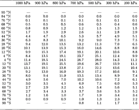
The distribution of NOt (Table 1) was based on an analysis of aircraft, shipboard and surface data for NO

and NOs. [e.g., Torres and Thompson, 1993; Carroll and

Thompson, 1995; Emroohs et al., 1997; Bradshaw et al., 2000]. Profiles for NOt in Table 1 were obtained using

observations of NO, that is, by ensuring that the peri-

odic solution of the system of kinetic equations repre- senting the full chemical mechanism (with a period of 24 hours) provides NO values in agreement with daytime observations for NO. In the continental boundary layer

in some regions, as described below, values for NOt de- rived in this manner were replaced using observations

of NOx.

In deriving vertical profiles for NO, we used the anal-

ysis of Bradshaw et al. [2000] who gridded data from the NASA Global Tropospheric Experiment (GTE) and Airborne Arctic Stratospheric Experiment (AASE) air- craft campaigns, supplemented by measurements from other campaigns [e.g., Drummond et al., 1988; ICondo et al., 1993; Rohrer et al., 1997]. Although these data

are not sufficient in spatial or temporal extent to define

a climatology for NO, they provide a series of "snap-

shots" that show some consistent patterns; for example,

concentrations of NO in the marine boundary layer are low, a few parts per trillion by volume (pptv), those

from 4 to 6 km tend to be in the range 10-40 pptv over both oceans and continents, while values for 10-12 km

are generally in the range 10 to 150 pptv. Over the polluted continents, boundary layer concentrations are

Table la. Distribution of NOt

90øS-30øN 30øN-90øN

Pressure, hPa Ocean Land Ocean Land

1000 11 67 23 184 900 13 65 28 155 800 13 57 25 117 700 22 47 34 83 500 31 33 53 56 300 93 94 172 176 200 135 137 224 247 150 129 131 - - 100 132 133 - -

Except (1) for the continental boundary layer over indus-

trial regions of Europe, North America and South-East Asia where i ppbv of NOt was assumed in summer and 2 ppbv

in winter, and (2) for tropical regions affected by biomass

burning where Table lb applies. Concentrations of NOt are in pptv.

Table lb. NOt in Biomass Burning Regions

Pressure, hPa Ocean • Land b

1000 12 219 900 33 223 800 45 213 700 55 125 500 70 70 300 219 220 200 275 276 150 262 260 100 260 257

Concentrations of NOt are in pptv.

•Over Atlantic (0ø-24øS) in July-October.

hover Africa and South America (0ø-24øS) in July-Octo- ber and over Africa (0ø-16øN) in November-March.

from 100 pptv to several parts per billion by volume

(ppbv), and the profiles are C shaped [e.g., Drummond et al., 1958], while in remote areas, such as the Ama- zon, concentrations are much lower, 10-40 pptv [Torres and Buchan, 1988]. Boundary layer concentrations in

remote regions affected by biomass burning are elevated

compared to those removed from such influence. Based on the features seen in the observations, we allowed for different profiles for NO over land and ocean, south and

north of 30øN, and for a region in the southern tropics

(0 ø - 24øS, 60øW- 45øE), with higher concentrations

over the latter region in austral winter-spring using ob-

servations from the Transport and Atmospheric Chem- istry Near the Equator-Atlantic (TRACE-A) mission.

The standard "land" and "ocean" profiles are identical

above 6 km.

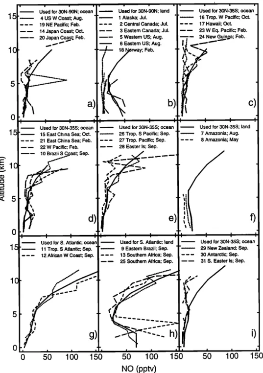
The profiles selected for NO are compared in Figure

1 to observations in various parts of the world [Brad- shaw et al., 2000; GTE data archives, 1998]. In addi- tion to the data shown in the figure (from which the selected profiles were largely derived), the ocean pro-

file for 30ø-90øN agrees well with measurements from

Stratospheric Ozone Experiment (STRATOZ) III from

the east coast of North America and the west coast

of Europe in June 1984 [Ehhalt and Drummond, 1988;

Drummond et al., 1988]; mean NO values for 20ø-70øN

were only 20% larger than the standard profile in Figure la for 3-8 km, and were about a factor of 2 larger for 10-12 km. Measurements from the Tropospheric Ozone

Experiment (TROPOZ) II in January 1991 [Rohrer et al., 1997] close to Europe-(not shown) were within a fa.c-

tot of 2 or less of the standard profile in Figure l a, but downwind of North America were much higher, 100-300

pptv for 2-6 km. For 30øN-90øN over land (Figure lb),

in addition to the data included in the figure, Ridleg et

al. [1994] observed values for NO as low as 20 pptv at

4-6 km over New Mexico in summer, similar to those

over the oceans, while values above 6 km were factors

of 2-3 higher than those in Figures la and lb, because of the bias in sampling near convective storms.

SPIVAKOVSKY ET AL.' CLIMATOLOGICAL DISTRIBUTION OF TROPOSPHERIC OH 8935 15 10 15 ,,,10 o_ • 5 i 1 '- ... 4 US W Coast; Aug. --- 19 NE Pacific; Feb.

--- 14 Japan Coast; Oct.

•

!

:

'---.- 1 Alaska;

Jul.

'/---

16

Trop.

W Pacific;

Oct.

--- 2 Central Canada; Jul. /--- 17 Hawaii; Oct.

--- 3 Eastern Canada; Jul. /• • 23 W Eq. Pacific; Feb.

--- 20 Japan C0a•,,st; Feb. •-- 5 Western US' Aug. /---- 24 New Gui.n,•a; Feb.

_ 6 Eastern US; Aug. I I J

"• •'

' '"-%J'•

18

•J,erway;

Feb. T •'. •

,,?-

/ /

I I I

I

' l•__•.•__

I

Used for 30N-35S; ocean Used for 30N-35S; ocean Used for 30N-$$$; land ' : 5 East China Sea; Oct. 26 Trop. S Pacific; Sep. ' 7' Amazonia; Aug.

_ _ l, 21 East China Sea; Feb. 27' Trop. Pacific; $ep. - - - 6 Amazonia; May -- -- 22 W Pacific; Feb. 28 Easter Is; $ep.

•-- I0 Brazil S Sep. • • ,, I )

'

,:

f)

"

d)

e) ,,

J Used

for

S,

Atlantic;

oceanL

15

__...•.

•2

African

W

Coast;

Sap.

/-•2

I I I I I

Used

9

Eastern

for

S.

Brazil;

Atlantic;

Sep.

land

' •-•.•_-

Used

29

New

for

Zealand;

30N-35S;

Sep.

ocean

1½- 5 0 /' 2 • •-' I t • ß

ß

/I

g --"•.,,,,J-''-

II'l•

a

50 1•0 150

50 100 156

50 100

NO (pptv)

Figure 1. Vertical

profiles

of NO. The heavy

solid

lines

show

the profiles

adopted

for three

regions,

land

and

ocean:

30øN-90øN,

90øS-30øN

(based

on

data

from

30øN-35øS),

and

the

South

Atlantic

region

affected

by biomass

burning

for 24øS-0øS,

between

60øW

and

45øE

in August-

October.

These

are compared

with observations

for 30øN-90øN,

(a) ocean

and (b) land;

for the

tropics,

35øS-30øN,

(c, d, and

e) ocean

and

(f) land;

for the South

Atlantic

region,

(g) ocean

and

(h) land;

(i) for

southern

midlatitudes

(the

same

profile

as

adopted

for 35øS-30øN,

ocean).

Profiles

compiled

from

observations

for subregions

are

taken

from

Wang

et al. [1998b],

where

the

regions

are

defined,

with

the addition

of data

from

PEM-Tropics

[Bradshaw

et al., 2000;

GTE

data

archives,

1998]

for which

the data

were

averaged

over

the following

areas:

tropical

South

Pacific

(region

26, 5øN-15øS,

170øE-130øW);

subtropical

South

Pacific

(region

27, 10øS-35øS,

170øE-145øW);

Easter

Island

(region

28, 10øS-35øS,

120øW-105øW);

New

Zealand

(region

29,

35øS-55øS,

170øE-170øW);

Antarctic

(region

30, 55øS-75øS,

170øE-170øW);

South

Easter

Island

(region

31,

35øS-55øS,

115øW-105øW).

The

profiles

from

the

subregions

are

averages

over

all NO

points

obtained

with solar

zenith

angle

of less

than 700

8936 SPIVAKOVSKY ET AL.: CLIMATOLOGICAL DISTRIBUTION OF TROPOSPHERIC OH The standard ocean profile of NO adopted for 30øN -

35øS is similar to or higher than NO observed in the

vicinity of Hawaii, in the western Pacific, and in the southern Pacific in September/October (Figures lc and

ld), while observations from the western Pacific in win- ter are somewhat higher than the standard profile (ex- cept in the middle troposphere). NO values reported for flights from Japan to Indonesia at 4.5 km (not shown) were about 20 pptv in continental plumes in winter and summer, but only 7 pptv in marine air near the equa- tor [Kondo et al., 1993]. The standard ocean profile

for 30øN-35øS is similar to mean profiles for these lat-

itudes derived from measurements made as part of Pa- cific Exploratory Mission (PEM)-Tropics [Bradshaw et al., 1999] (Figure le). The NO profile selected for land

in the tropics is based on longitudinal transects from

Arctic Boundary Layer Expedition (ABLE) 2A over much of the Amazon [Torres and Buchan, 1988], while observations in Figure if are for the area around Man- aus only. Mean values for NO from TROPOZ II data are 20-60 pptv for 4-8 km between 30øS and 30øN over

the Americas,

higher

than the standard

profiles

(not

shown). The NO profiles

selected

for tropical regions

affected by biomass burning are based on limited data available from TRACE-A (Figure lg for the Atlantic

Ocean,

and Figure lh for the adjoining

continents).

The land profile for NO for regions of Africa and South America affected by biomass burning in June - Octo- ber was used over sub-Saharan Africa for the biomass

burning season in November- March.

We chose to use the NO profile for 35øS to 30øN for

southern midlatitudes prior to the availability of data

from PEM-Tropics A and TROPOZ II. The measure- ments from PEM-Tropics A south of 35øS tend to show

lower concentrations

of NO than the standard

profile,

by about a factor of 2 below 5 kin, and by as much

as a factor

of 2-6 at 8 km and above

(Figure

li). How-

for southern

midlatitudes,

by up to a factor

of 3 (not

shown). These differences

may reflect seasonality

in

sources of NO•:, but data are insufficient to resolve this

uncertainty.

Below 300 hPa, NOt is present primarily as NOx, ex-

cept in winter at temperate latitudes. Concentrations

of NO•: (and NO) are highly variable in surface air over the northern continents. The NO value near the sur-

face selected

for the standard

profile

in Figure lb cor-

responds to about 180 pptv of NO•:. Concentrations of

NO•: reported for remote locations in the United States

and Nova Scotia are --•100-300 pptv, while median val- ues at more polluted rural sites in the eastern U.S. and

Canada

are 1-2 ppbv in summer,

with somewhat

higher

values in winter; mean values are higher than median

values

[Carroll and Thompson,

1995; Emroohs

½t al.,

1997; Munger et al., 1998]. In the boundary layer over

industrial regions of Europe and North America we as-

sumed 1 ppbv of NOt in summer and 2 ppbv in winter.

Concentrations

of NOt adopted

for this study are

higher

than in S90 by factors

of 2-5 in the tropics

over

regions affected by biomass burning and over industrial

regions

at northern

midlatitudes.

In addition,

concen-

trations

of NOt below

800 hPa over oceans

are higher

in the present

work, by factors

ranging

from 1.5 to 2.

The changes in the distribution of NOt resulted in an

increase

of--•7% in mean OH as compared

to S90.

2.4. Carbon Monoxide

For CO we took an approach different from that for

03 and NOt. There was no published 3-D climatol- ogy for CO as was the case for 03, and in contrast to NOt, for CO there was a wealth of surface observa-

tions and, in some locations, column observations. We

used the CTM as an interpolator to obtain a smooth

distribution of CO consistent with observations. For

this purpose

the inventory

of emissions

presented

by

Wang

et al. [1998a]

was

adjusted

to provide

satisfactory

agreement with observations of CO from NOAA Cli-

mate

Monitoring

and Diagnostics

Laboratory

(CMDL)

and

other

surface

sites

[Novelli

et al., 1998;

W. Munger,

personal

communication,

1997;

Schcel

et al., 1990],

and

where available, with observations of the CO column

[Dvorgashina

et al., 1984;

Zander

et al., 1989;

Rinsland

et al., 1998]

(using

the distribution

of OH from

S90).

The agreement between observations and the distribu-

tion of CO specified in the present calculation of OH is

illustrated

in Figures

2a, 2b and 2c for surface,

column,

and aircraft data, respectively.

Specified values for CO are consistent with GTE air-

craft

observations

over

the tropical

Pacific

and

Atlantic,

as well as off the west coast of South Africa and east

coast

of Southern

Brazil (Figure

2c). Model levels

are

also in agreement with observations over Kansas and

Maine. Good agreement was also found at southern

middle

and high latitudes

over the Pacific

in Septem-

ber, but values over New Zealand are too low above

500 hPa. Over the Hawaiian

region,

specified

values

are higher

than observations

by 20-35%

in January

but

are in agreement in August. Over the West Coast of the

United

States

both

in winter

and

summer

(not

shown)

as well as off the coast

of Japan and China specified

values are too high.

We also compared the adopted distribution of CO

with satellite observations, Measurement of Air Pol-

lution from Satellites (MAPS), which give the major weight to the region between 500 and 250 hPa, for

10 days in April and October (not shown). In April,

model levels are consistent with observations, except

at southern midlatitudes where the former are too low

by as much as 35%. In October, the same discrepancy is evident at southern midlatitudes, and in addition,

she biomass burning plumes in the SH are much less

pronounced in the model than in MAPS observations,

consistent with the underestimation of the column data

of Rinsland

et al. [1998]

for October (Figure 2b) at

SPIVAKOVSKY ET AL.' CLIMATOLOGICAL DISTRIBUTION OF TROPOSPHERIC OH 8937 250 150 50_1.: : : : : : : :: : : :.• ... •. ... .I. ...

Shemya_ls_AK

(52N,

1741•

....

250••

St_David_Berm_S (32N, Canary_Is (28N, 16W) Midway_Is (28N, 177VV) Key_B[scayne_FL (25N, 25O

150 50 125

Mauna_Loa (19N, 155W) (13N, 14.4E) Barbados (13N, 59W) Christmas_Is (1 N, 157%0

75

25., , , : : : : : : : : :' ,

1251N-Seychelles

(4S,

55E)

Asc-lsland

(7S,

14W)

'Samoa

(14S,

170W)

[Easter-Is

(29S,

109W)

t

75

•,i, 2•,•

,i, - -"•_•,o

100

Cape_Point

(34S,

18E) Cape_Grim

(40S,

144E)

Palmer_Stn

(64S,

60W)

South•Pole

(90S,

0W) "

75 50

25 ß

J M M J S N J M M J S N J M M J S N J M M J S N

Month

Figure 2. Comparison

of model

results

(lines)

used

to specify

the global

distribution

of CO with

observations

at selected

sites

(a) at the surface,

(b) for the column,

and (c) using

aircraft

data

from GTE campaigns. For the surface, open circles, solid circles, and squares denote observations

of Novelli et al. [1998],

Scheel

et al. [1990],

and W. munger

(personal

communication,

1997,

averages

over 1990-1994),

respectively.

For the column,

squares,

triangles

and diamonds

refer

to observations

of Dvoryashina

et al. [1984],

Zander et al. [1989],

and Rinsland

et al. [1998],

respectively.

For the aircraft data, profiles

where

compiled

using GTE data archives

for regions

defined in caption for Figure 1, with the exception of Hawaii, region 32, 15øN-25øN, 155øW -

165øW,

from the Stratospheric

Tracers

of Atmospheric

Transport

(STRAT) mission;

Kansas,

region 35, 35øN-40øN, 94øW-101øW, from Subsonic Aircraft Contrail and Cloud Effects Special

Study; Maine coast, region

36, 41øN-50øN,

55øW-72øW;

and Ireland, region 37, 49øN-54øN,

3øW-13øW

from Subsonic

Assessment

(SASS)

Ozone

and Nitrogen

Oxide

Experiment

(SONEX).

Means are denoted by asterisks, medians are shown as vertical lines inside boxes, 25% and 75% quantties are represented by boxes, and 10% and 90% quantties are marked by dots.

8938 SPIVAKOVSKY ET AL.' CLIMATOLOGICAL DISTRIBUTION OF TROPOSPHERIC OH

c)

26 Tro'p.S.Pacifi½

b) so

• lO

"

J FMAMJ J ASONDJ FMAMJ J ASOND

Month

23 W.Eq. Pacific

February

27 Trop. Eq. Pacilic September ß 32 Hawaii

"--. January

'15 East China Sea

October 29 New Zealand September 50 150 250 CO (ppbv) 16 Trop. W.Pacific October ß 10 BraziI.S.Coast September 14 Japan Coast October 30 Antarctic September 50 150 250 Figure 2. (continued) ß •'8 I•as{er is September 12 African W.Coast September , I I I I 36 Maine Coast October -I' 31 S. Easter Is September

Concentrations of CO used in this study are about

20% lower in the SH and in the northern tropics as

compared

to S90 [cf. Manning et al., 1997], resulting

in an increase of--•7% in global mean OH. It is possi-

ble, however, that an underestimate of CO at southern

midlatitudes suggested by the MAPS data contributed

to an overestimate of OH in that region discussed in

section 9.

2.5. Hydrocarbons

The methane field was assumed uniform in each semi-

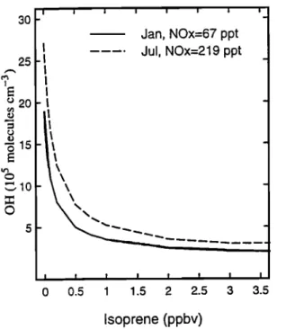
SPIVAKOVSKY ET AL.: CLIMATOLOGICAL DISTRIBUTION OF TROPOSPHERIC OH 8939 3O 25 i I i I I i i I_ . Jan, NOx=67 ppt

. I

I

....

Jul,

NOx=219

ppt _

-I

-

Isoprene (ppbv)

Figure 3. Concentration

of OH (10

s molecules

cm

-3)

at the surface at 15øS versus concentration of isoprene

in January,

with NOt at 67 pptv (solid

line) and in July,

with NOt a,t 219 pptv (dashed line). NO.• constitutes more than 99.% of NOt.

1655, 1715, and 1770 ppm, respectively [Dlugokcnck•l ½t al., 1994, 1995] (for the present resolution, actual divisions are at 32øS, the equator and 32øN).

Isoprene provides a major sink for OH near the sur-

face over land in the tropics and at midlatitudes in sum-

mer [e.g., Greenberg

½t al., 1985; Zimmerman

½t al.,

1988; Jacob and Wofs9, 1988]. Concentrations of iso-

prene, however,

are highly variable

in space

and time,

and measurements are few. We specified the distribu-

tion of isoprene simulated using the model of Horou•itz

and Jacob

[1999]. Emissions

of isoprene

were reduced

for tropical forests and grassland by factors of 2 and 3, respectively, and increased for "snowy mixed" forests

(terminology

from Guenther

et al. [1995])

by a factor

of 3. In these modifications we were guided by com-

parisons

of model results

with observations

for vertical

profiles of isoprene [t•asmusscn and I(halil, 1988; Jacob and Wofsy, 1988; Ayers and Gilett, 1988; Andronache et al., 1994; Guenther et al., 1996; Helmig et al., 1998; GTE data archives, 1998]. For tropical forests, such a

decrease in emissions is also supported by direct esti-

mates of Jacob

and Wofsy

[1988, 1990] and Ii'lin9er et

al. [1998]. In addition,

emissions

for "dry taiga" were

reduced by a factor of 3 (A. Guenther, personal com-

munication, 1998).

Over large regions, however, concentrations of iso- prene are highly uncertain. Nevertheless, for isoprene above .-•250 pptv, OH is depleted by more than a factor of 2, as shown in Figure 3, and therefore uncertain-

ties in concentrations of isoprene above that level do

not contribute significantly to those in the tropospheric column of OH. At concentrations of isoprene above 500 pptv, the sensitivity of OH to isoprene is greatly di- minished because production of OH is dominated by

photolysis of products of isoprene oxidation, such as

CH20 and organic peroxides. As a result, a larger un-

certainty in OH is associated with the spatial extent of concentrations of isoprene in excess of 50-100 pptv than with the accuracy of the specified values above 500 pptv. The lifetime of isoprene away from imme- diate sources is counted typically in hours. Little er- ror is expected to result therefore from uncertainties in the horizontal transport in the CTM. However, verti- cal transport within the boundary layer may be more rapid than chemical loss, and therefore the vertical ex-

tent of significant levels of isoprene is sensitive to errors in the height of the boundary layer and the frequency of

convection in the CTM [Horowitz and Jacob, 1999]. An

additional uncertainty in OH is associated with the spa-

tial extent of significant concentrations of longer-lived

intermediate products of isoprene oxidation, for exam- ple, methacrolein and methylvinylketone, since our cal- culation of OH neglects the effect of transport of these compounds by forcing their concentrations to a peri- odic steady s•ate. Model results for isoprene with the 40 by 50 resolution on •r surfaces were adopted for the 80 by 100 resolution on standard pressure levels using linear interpolation in the logarithm of isoprene because of the highly nonlinear dependence of OH on isoprene. Concentrations of isoprene were specified with the time resolution of a month, with averaging in time conducted also for the logarithm of isoprene. Inclusion of isoprene

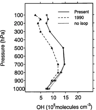
decreased global tropospheric OH by 3%. For the dis-

tribution of isoprene obtained using standard emissions

from Horowitz and Jacob [1999] rather than reduced

emissions, and with interpolation and averaging con-

ducted for concentration (rather than for logarithm of concentration), global tropospheric OH decreased by

9%.

Apart from isoprene and methane, we considered

12 hydrocarbons: alkanes (C2H6, C3H8, C4Hlo, and can•2), alkenes (Cull4 and c3n6), aromatics (c6n6,

C7H8, and CaHlo), and oxygenated

species

(re_ethanol,

ethanol, and acetone). Using observations, we devel-

oped concentration profiles for four latitude regions, two

seasons, and for land and ocean, and determined which

species needed to be included in the calculation of global

OH with a series of sensitivity studies.

Measurements of hydrocarbons are most abundant

for northern midlatitudes. Values selected for the conti-

nental boundary layer were based primarily on the data

from surface sites shown in Table 2 and were chosen

to represent background conditions; values above the

boundary layer in summer were based on data obtained

near North Bay, Canada. Median vertical profiles were

calculated for each hydrocarbon species for selected ge-

ographic regions, using the GTE data merges provided

by Bradshaw ½t al. [2000]. The marine profiles were

8940 SPIVAKOVSKY ET AL.: CLIMATOLOGICAL DISTRIBUTION OF TROPOSPHERIC OH

Table 2. Data for Alkenes and Alkanes at Northern Midlatitudes

C2H4 C3Ho C2Ho C3H8 C4H10 CsHla C4+Cs Ce Ref.

Averages for JJA, Surface Stations

Kejimkujik • 160-190 70-90 1080 243 153 170 323 200 1 Lac la Flamme • 120-210 50-60 1030 140 60 73 133 150 1 Egbert • 170-300 50-70 1130 300 233 217 450 200 1 Saturna • 220-260 60 970 310 273 233 406 170 1 Fraserdale • ND ND 820 78 22 8 ND 2 Rorvik, Sweden 213 34 817 215 381 243 624 ND 3 Harvard Forest b 485/179 119/55 1537/959 663/265 419/116 533/153 952/269 107/40 4

Averages for JJA, Aircraft Data

ABLE-3A ND ND 820 49 8 (n-C4) 5

ABLE-3B c 78/51 21/10 853/703 92/79 49/35 LOD/LOD 6 PEM-A d 64/89 17/21 1021/1601 153/540 88 33 124/487 7(n-C6) 7 PEM-A e 29/30 14/8 632/1019 57/154 20 13 34/101 LOD 7

Selected for Northern Midlatitudes, JJA

160 60 1000 250 300 40

Averages for D JF, Surface Stations

Kejimkujik • 300-530 60-170 2230 1350 1040 523 1560 340 1 Lac la Flamme • 300 30-60 2370 1310 930 450 1380 280 1 Egbert • 460-1230 60-160 3130 2080 1790 840 2630 370 1 Saturna • 1000 60-210 2130 1160 1730 790 2520 42 1 Fraserdale • ND ND 2450 1140 930 490 ND 2 Rorvik, Sweden 995 172 2620 1316 1360 942 2310 ND 3 Harvard Forest b 1112/402 181/45 3420/2290 1980/1170 1510/734 849/405 2358/1139 192/95 4 Atlantic 2200 850 600 320 920 100 8 (nC6+C7) PEM-B f 86/90 7/7 2258/2283 877/900 34 553/580 37/40 9 400 45

Selected for Northern Midlatitudes, DJF

2200 1150 1150 100

For PEM-West A and B, the first number shows the median of all measurements below 1 km for the selected region,

and the second number shows the median for C• • 750 pptv (PEM-A) and for C•H6 • 1000 pptv (PEM-B). ND, no data.

LOD, below detection limit. JJA, June, July, August; DJF, December, January, February. References are 1, Bottenheim and Shepherd [1995]; 2, Jobson et al. [1994]; 3, Lindskog and Moldanova, [1994]; 4, Goldstein et al. [1995b]; 5, Blake et

al. [1992]; 6, Blake et al. [1994]; 7, Blake et al. [1996b]; 8, Penkerr et al. [1993]; 9, Blake et al. [1997]. Concentrations of

hydrocarbons are in pptv.

• Canadian stations.

bThe first and second number correspond to a mean and a 10th percentfie, respectively. CThe first and second number correspond to values at North and Goose Bay, respectively.

dNear the coast, north of 23øN. eEast of 143øE, north of 23øN.

f North of 2 IøN.

from the western Atlantic [Penkett ½t al., 1993], and from the eastern Pacific north of 21øN (PEM-West A);

for PEM-West A a filter of C2H6 > 750 pptv was used

to select midlatitude air.

Winter profiles were selected for northern midlati- tudes in the same manner as for summer, but the air- craft data were limited to the western Atlantic and the

eastern Pacific (PEM-West B), and a few profiles mea- sured in the vicinity of California [$ingh ½t al., 1988].

We used a filter of C2H6 > 1000 pptv to select midlat-

itude values

from PEM-West B (for latitudes

> 21øN)

and used these values above 3 kin for land and for the entire profile for ocean; this resulted in profiles similar

to those reported by $ingh et al. [1988] and Rudolph

[1995] for the alkanes. Concentrations of alkenes in the

marine boundary layer, which are short lived even in

winter, were taken from Rudolph

and Jobhen

[1990].

Vertical profiles for the tropics were derived largely

from PEM-West

A (10øN-22øN)

and B (7.5øN-21øN)

in the eastern Pacific, TRACE-A in the South Atlantic,

Brazil, and Africa, three cruises

in the Atlantic [$ingh

et

al., 1988; Rudolph and Jobhen, 1990; Koppmann et al.,

1992], two in the Pacific [$ingh et al., 1988; Donahue

and Prinn et al., 1993], and continental measurements in Africa and Brazil [e.g., Zimmerman et al., 1988; Rudolph et al., 19923]. Profiles above the boundary

layer in the northern tropics were based almost exclu-

SPIVAKOVSKY ET AL.: CLIMATOLOGICAL DISTRIBUTION OF TROPOSPHERIC OH 8941

surements on TRACE-A transit flights; in the southern

tropics,

they were based

on TRACE-A data for Octo-

ber, and on PEM-West B data near the equator

for

February.

Continental

data were

lacking

for the north-

ern tropics,

so the southern

data were

used

to estimate

concentrations in the wet and dry season. The conti-

nental data are much cruder estimates of typical values

as the measurements are for short time periods, usually

a few weeks at most. Relatively few vertical profiles

•ere measured over the continents during TRACE-A,

and they appear reasonably consistent with the surface data from the dry season reviewed by Rudolph et al.

Profiles derived for southern midlatitudes were based on measurements from cruises to ---30øS [Rudolph and Johnen, 1990; Koppmann et al., 1992] and vertical

profiles

from TRACE-A that sampled

midlatitude

air,

based on backward trajectory calculations. These data

gave

lower concentrations

of alkanes

than surface

data

from 70øS reported by Rudolph et al. [1992b] but were

thought

to be more representative

of middle latitudes.

The concentration profiles for hydrocarbons are most

reliable for alkanes, and the reliability decreases for

aromatics and oxygenated species, simply because of the quantity of measurements; for short-lived hydrocar- bons, such as alkenes, the high spatial and temporal variability results in greater uncertainties. The profiles

are better known for June to October than for Decem-

ber to March, because of the timing of the aircraft cam-

•paigns,

and for northern

midlatitudes

compared

with

any other region, because of the availability of surface data, and of several sets of aircraft data. While the

vertical profiles selected for the tropics are less defined than those for northern midlatitudes, there appears to

be reasonable consistency among the tropical measure-

ments as shown in Table 3 for alkenes.

Surface measurements of benzene and toluene were

available for only a few remote surface sites and cruises [Rasmussen and Khalil, 1983; Nutmagul and Cronn,

1985; Dann and Wang, 1995], in addition to measure-

ments from aircraft campaigns [Penkett et al., 1993;

Blake et al., 1994, 1996a, b, 1997]. Concentrations of

toluene and xylenes were often below detectable levels (2 pptv) in the SH [Blake ½t al., 1994, 1996a, b]. We

found that at present levels reactions involving aromat- ics have an impact of less than 2% on computed concen- trations of OH over most of the globe. Given that in- clusion of aromatics adds significantly to computational

cost, we chose to exclude them from our calculation [cf.

Houweling et al., 1998].

Acetone was measured on the GTE campaigns in

eastern Canada, the eastern Pacific (February-March),

and the south tropical Atlantic, ethanol on the last two

of these, and methanol in the eastern Pacific [Singh et al., 1994, 1995, 1996a]. Acetone concentrations for

northern midlatitudes were about the same in sum-

mer and winter, ---600 pptv. Methanol concentrations were also about 600 pptv in northern winter, but data

for other seasons were lacking. Ethanol concentrations

were smaller, 50-80 pptv in the NH and below the limit of detection (20 pptv) in the SH in October.

Omission of isoprene and other NMHCs results in an

increase in global tropospheric OH by 3% and 7%, re- spectively [cf. Donahue and Prinn et al., 1993; Houwel-

Table 3. Near Surface Data for Alkenes

Location Season C2H4 C3H6 Reference

Northern Tropics

Atlantic cruise Sep./Oct. 30 ND 1

Pacific aircraft (10øN-22øN) Oct. 20 8 2

Pacific aircraft (0ø-10øN) Oct. 24 8 2

Atlantic cruise Mar./Apr. 70 15 3

Pacific cruise (0ø-10øN) Feb./Mar. 60 50 4 Pacific aircraft (7øN-21øN) Feb./Mar. 7 4 5

Selected for Oct. 30 12

Selected for Feb. 65 32

Southern Tropics

Atlantic cruise Sep./Oct. 22 ND 1

Atlantic aircraft Oct. 13 4 6

Atlantic cruise Mar./Apr. 25 10 3 Pacific cruise Feb./Mar. 45 40 4

Pacific aircraft Feb./Mar. 7 LOD 5

Selected for Oct. 22 10

Selected for Feb. 35 25

Aircraft data are shown as median values from •300 m to 1000 m. References are

1, Rudolph and Jobhen [1990]; 2, PEM-A, Blake et al. [1996b]; 3, Kopprnann et al.

[1992];

4, Donahue

and Prinn [1993];

5, PEM-B, Blake et al. [1997];

6, TRACE-A,

D. R. Blake, personal communication (1996). ND, no data; LOD, below detection limit.