Opening a Pandora’s Box: Modeling World Trade Patterns at the 2035 Horizon

HAL Id: hal-01299851

https://hal.archives-ouvertes.fr/hal-01299851

HAL is a multi-disciplinary open access archive for the deposit and dissemination of sci-entific research documents, whether they are pub-lished or not. The documents may come from teaching and research institutions in France or abroad, or from public or private research centers.

L’archive ouverte pluridisciplinaire HAL, est destinée au dépôt et à la diffusion de documents scientifiques de niveau recherche, publiés ou non, émanant des établissements d’enseignement et de recherche français ou étrangers, des laboratoires publics ou privés.

Opening a Pandora’s Box: Modeling World Trade

Patterns at the 2035 Horizon

Lionel Fontagné, Jean Fouré

To cite this version:

Lionel Fontagné, Jean Fouré. Opening a Pandora’s Box: Modeling World Trade Patterns at the 2035 Horizon. 2013. �hal-01299851�

1

Staff Working Paper ERSD-2013-09

Date: August 02, 2013

World Trade Organization

Economic Research and Statistics Division

Opening a Pandora’s Box:

Modeling World Trade Patterns at the 2035 Horizon

Lionel Fontagné & Jean Fouré

Manuscript date: August 2, 2013

___________________________

Disclaimer: This is a working paper, and hence it represents research in progress. This paper

represents the opinions of the author(s), and is the product of professional research. It is not

meant to represent the position or opinions of the WTO or its Members, nor the official

position of any staff members. Any errors are the fault of the author(s). Copies of working

papers can be requested from the divisional secretariat by writing to: Economic Research and

Statistics Division, World Trade Organization, Rue de Lausanne 154, CH 1211 Geneva 21,

Switzerland. Please request papers by number and title.

2

OPENING A PANDORA’S BOX:

MODELING WORLD TRADE PATTERNS AT THE 2035 HORIZON

Lionel Fontagné

& Jean Fouré

August 2, 2013

ABSTRACT

Economic projections for the world economy, particularly in relation to the construction of Computable General Equilibrium (CGE) baselines, are generally rather conservative and take scant account of the wide range of possible evolutions authorized by the underlying economic mechanisms considered. Against this background, we adopt an ‘open mind’ to the projection of world trade trajectories. Taking a 2035 horizon, we examine how world trade patterns will be shaped by the changing comparative advantages, demand, and capabilities of different regions. We combine a convergence model fitting three production factors (capital, labor and energy) and two factor-specific productivities, alongside a dynamic CGE model of the world economy calibrated to reproduce observed elasticity of trade to income. Each scenario involves three steps. First, we project growth at country level based on factor accumulation, educational attainment and efficiency gains, and discuss uncertainties related to our main drivers. Second, we impose this framework (demographics, gross domestic product, saving rates, factors and current account trajectories) on the CGE baseline. Third, we implement trade policy scenarios (tariffs as well as non-tariff measures in goods and services), in order to get factor allocation across sectors from the model as well as demand and trade patterns. We show that the impact of changing baselines is greater than the impact of a policy shock on the order of magnitude of changes in world trade patterns, which points to the need for care when designing CGE baselines.

JEL Classification: E23, E27, F02, F17, F47

Key Words: Growth, Macroeconomic Projections, Dynamic Baselines

* PSE (Paris 1) and CEPII. Email: lionel.fontagne@univ-paris1.fr

‡

3 INTRODUCTION

What will be the main patterns of world trade in the 2030s? This is an important question since it refers to whether the institutional environment of international trade will produce a level playing-field. There is much uncertainty in such projections. There are two main sources of errors of judgment: projection of the drivers of international trade, and the basic unpredictability of some key variables which is an irreducible source of error.

Thus, it is essential to properly project the drivers of international trade: conditional on trade frictions and prices, the volume of trade is basically a function of countries’ Gross Domestic Product (GDP), according to the extensively documented principle of gravity. The key here is to have a sound representation of economic growth, providing GDP projections for the largest number of world countries. Is it best to adopt a very detailed model of growth that includes regulations for example, or a detailed representation of the public sector, or to focus on the main mechanisms and treat national idiosyncrasies as unobservable? There is a trade-off between restricting projections to the set of OECD countries (plus a handful of emerging economies), and including a much larger set of countries in a more stylized growth model.

The second prerequisite is to acknowledge the unpredictability of certain key variables. Energy prices could vary widely over the next 20 years, not primarily as the result of uncertainties surrounding economic growth, but due to geopolitical tensions (e.g. Middle-East) or technological breakthroughs (e.g. shale gas or jumps in energy efficiency). Female participation in the labour force is expected to increase as countries develop, but this driver of growth is also subject to uncertainties. Education convergence may speed up or may be hampered, with sizeable impacts on productivity. The future of international capital mobility is also very uncertain. Productivity convergence may accelerate or decelerate as a result of methods of technology transfer and approaches to firm mobility. Lastly, we may observe large migrations flows as a result of unexpected push factors, while fertility rates are highly uncertain.

Against this background, this paper has a methodological aim. First, to demonstrate how to feed into a dynamic sectoral model of the world economy projected economic growth for a larger set of countries. These projections use a stylized conditional convergence model of economic growth fitting three factors (capital, labor and energy), two types of technological progress (total factor productivity – TFP – of the capital-labor combination, and energy efficiency) and international capital mobility. We also project saving rates (based on a life cycle hypothesis) and current accounts. GDP and saving are projected at the country level, while constraints are imposed in terms of global balance between saving and investment. The second aim is to illustrate how induced GDP, saving, energy efficiency and current account trajectories to 2035 can be imposed on a Computable General Equilibrium (CGE) model of the world economy, relying on identical assumptions about population, labor force, education and current accounts. The CGE, in turn, will provide factor allocation (across sectors), demand patterns (preferences and budget shares) and, thus, trade patterns, conditional on trade costs. In addition to illustrating step by step how best to combine the modeling tools, our exercise adopts open-minded assumptions about the evolution of the key drivers of growth. For example, we give free rein to economic mechanisms, hence opening a Pandora’s Box of growth projections. We examine the impact on economic growth of large and combined shocks to its main drivers. Not all shocks will affect developing and developed economies in the same way. We combine the effects of these shocks with possible evolutions in trade costs. In addition to energy prices, we consider the situation of a tariff war driving countries beyond the legal World Trade Organization (WTO) framework, to post-Tokyo Round tariff levels. We examine the impact of generalized inspection of shipments, as a response to pandemics or terrorism. Finally we address changes in the barriers to services trade. The

4

aim is not to suggest that any of these scenarios is plausible given current information on the world economy. Instead we want to show how common modeling tools can be combined to characterize the broad range of possible world trade patterns associated with the presence of high uncertainty. We conclude that the impact of changing baselines is greater than the impact of a policy shock on the order of magnitude of changes in world trade patterns, which points to the need for care when designing CGE baselines.

This methodological paper contributes to a recent and growing body of literature on long term prospects for the world economy. Qualitative scenarios combining the two modeling frameworks as a background to a more multidisciplinary approach centered on Europe were developed at the 2050 horizon for the European Commission (EC, 2012). The International Monetary Fund (IMF, 2011) uses a partial equilibrium approach to address the consequences of reductions in exchange rate misalignment with trade patterns in the presence of global value chains and possibly imperfect pass through. Fontagné et al. (2013) proposes possible scenarios to be used as background for environmental studies, and considers the 2100 horizon in order to explore methodological issues associated with the use of long term dynamic baselines in CGE models. World Bank (2007), which is closer to our approach, relies on a multisectoral model of the world economy comparable to MIRAGE, to sketch scenarios for the world economy at the 2030 horizon. None of these studies use an explicit growth model and the scenarios are driven by assumptions about TFP imposed on the CGE. In contrast, Petri and Zhai (2013) rely on Asian Development Bank growth projections using a growth model similar to ours (ADB, 2011). They use this GDP series to derive scenarios at the 2050 horizon, with a CGE model on which assumptions about TFP, higher food prices, higher energy prices, or protectionism are imposed. Finally, Anderson and Strutt (2012) consider the 2030 horizon and build a baseline for the GTAP CGE model by drawing on both ADB (2011) and Fouré et al. (2010).

The value added of the present paper is to highlight the technical issues and the wide range of uncertainty raised by combining macroeconomic and multisectoral models which open a Pandora’s box of long term projections. For example: (i) it builds scenarios for some 150 countries, taking account of the interactions among capital mobility and trade in goods and services; (ii) it implements scenarios in a consistent way in both the growth (Macroeconometrics of the Global Economy – MaGE) and multisectoral dynamic CGE (MIRAGE) models; (iii) the scenarios tackle a wide range of potentialities paying close attention to decomposition of effects. To our knowledge, this is, the only exercise so far on such a scale, at the 2035 horizon, adopting a methodology of consistent scenario construction for the growth and the CGE models.

The rest of the paper is organized as follows. Assumptions related to growth projections and our scenarios are presented in Section 1. Section 2 describes the methodology and the scenarios are implemented in the growth model in Section 3. Section 4 summarizes the results of the global and sectoral models of the world economy. The last section concludes.1

1 _{A companion paper discusses our main findings in depth: Fontagné L., Fouré J. and A. Keck (2013), Simulating}

5

1. MODELING GROWTH PROJECTIONS AND DESIGNING SCENARIOS FOR THE WORLD ECONOMY

This paper is positioned at the junction between three strands of the applied economic literature: (i) economic growth projections; (ii) design of dynamic baselines in applied general equilibrium modeling with a focus on the environment; and (iii) design of medium and long term scenarios for the world economy. The first two are not independent: design of dynamic baselines relies on the first literature strand (GDP driven baselines), or provides GDP projections directly based on assumptions about changes in sector-specific TFP (TFP driven baselines). The third stream of literature combines quantitative elements (potentially provided by projections and baselines) with qualitative and sometimes multidisciplinary expertise on the main drivers of economic, social and environmental change. Below, we briefly survey the literatures related to growth projections, dynamic baselines and scenario building.

1.1. Growth projections

Increased interest in long-term economic-related issues, such as environment depletion and energy scarcity, has motivated several growth projection exercises. The business community initiated documentation of the huge shift towards the emerging economies (Wilson and Purushothaman, 2003; Ward, 2011), which was added to by work from international institutions. With some exceptions (Duval and de la Maisonneuve, 2010, Johansson et al., 2012), academic work in this area was sparse, leading to a lack of well-documented and economically-grounded projection models. This can be explained by the huge uncertainties surrounding projections that rarely prove accurate and are conditional on changes in the geopolitical context. Nevertheless, long-term investigations are a prerequisite for much downstream analysis, such as provided in this paper to address future patterns of world trade.

This lack of attention contrasts with the importance of economic growth factors in the economic literature. Starting from the standard neo-classical Solow model, mechanisms for production factor accumulation have been identified, for instance, in the demographic determinants of saving (see, for instance, Masson et al., 1998) and capital formation (Feldstein and Horioka, 1980), or in human capital catch-up and productivity improvements (Aghion and Howitt, 1992). Long-term growth projection models build on this vast literature by combining existing analyses.

At least three drivers are common to all empirical studies: capital stocks, labour force and TFP. These factors are taken into account by Wilson and Purushothaman (2003), which combines existing labour force projections, constant investment rates, and a convergence scenario for TFP. Duval and de la Maisonneuve (2010) identify human capital per worker as a driver, and calibrate conditional convergence scenarios among countries for each of these four determinants. Using a similar framework, Johansson et al. (2012) restrict their analysis to a smaller number of countries, but emphasize the impact of structural and fiscal policies (retirement age, trade regulation, public debt, credit availability). Finally, Fouré et al. (2013) introduce energy as a production factor along with energy-specific productivity, and base their projection framework on econometric analysis of both convergence mechanisms and structural relations. Comparing the projections in these papers we observe sizeable differences in the results. In Fouré et al. (2013), the share of China in world GDP at 2050 is almost twice the share projected by Duval and de la Maisonneuve. These differences call for transparency in assumptions and modeling frameworks and ’open-minded’ scenarios when introducing projections into dynamic CGEs.

6 1.2. Dynamic baselines

Large scale policy simulations generally rely on multisectoral dynamic models of the word economy. CGE is the most commonly used modeling framework. Policies are simulated as shocks and then the deviation of the variables of interest from their reference trajectory is computed. It could be argued that the modeler’s interest is in the deviation, not the initial equilibrium. However, this would be flawed reasoning if the focus is medium or long run policies: an economic policy affecting China would have a dramatically different impact on the world economy were China twice as large, which will be the case in less than ten years at current growth trends.

Since the model is exploited to determine capital accumulation, energy and primary resources prices, it is necessary to supplement it with world data including demographics. However, since CGE models generally do not describe the intrinsic mechanisms of growth (conditional convergence) they provide neither a satisfactory representation of efficiency gains from combining production factors, nor plausible trajectories for countries at different levels of development. Accordingly, it is necessary to constrain the CGE to reproduce a pre-defined GDP growth path or a pre-defined TFP path for each world country (or region). This is the aim of dynamic baselines.

Many baselines focus on the period up to 2020 (e.g. the GTAP model), but some exercises extend to 2050 (e.g. the Linkage model). Relying on an ambitious approach, Fontagné et al. (2013) tentatively consider the 2100 horizon in order to provide environmental studies with a theoretically consistent baseline of the world economy. Whatever the horizon, the building blocks of a baseline are the same. The first step is projection of a general trajectory of world growth, based on simple and robust economic mechanisms. There are two competing approaches to CGE modelling. The first option is to build a scenario for factor productivity growth in order to recover GDP from the CGE model. The second is to build a GDP scenario such that the model recovers the relevant TFP gains.

Recovering GDP from TFP growth assumptions has the advantage that availability of detailed data on demographics or education is not a limiting factor. Moreover, it allows different sector specific trajectories to be encompassed without over-constraining the model. However, this approach is very sensitive to assumptions related to TFP growth and its determinants. For instance, the EPPA model (Paltsev et al., 2005) assumes identical logistic productivity growth for all countries and sectors, and does not implement capital productivity.

The symmetric approach of imposing GDP growth trajectories onto a CGE, and recovering the productivity gains, is more data demanding since it is necessary, first, to project growth for every country. Its main advantage is that it enables proper modeling of growth by taking account of conditional convergence and possibly different types of technical progress, in line with the vast literature on macroeconomic growth. This is a very important advantage if the interest is in long run modeling of different kinds (mature, emerging, developing) of economies. Also, this approach allows greater reliance on the macro projections in the literature (see Fouré et al., 2013 for a short review). For instance, the main projections used in the GTAP model and earlier versions of MIRAGE (Decreux and Valin, 2007) were provided by the World Bank (Ianchovichina and McDougall, 2000).

The only crucial assumption in GDP-driven CGEs is the relative dynamism of productivity in broad sectors. Several approaches to this difficult issue have been proposed. The LINKAGE model (Van der Mensbrugghe, 2006-a) adds a sector-specific component – labor-only productivity – to endogenous national TFP. This approach results in: (i) a constant exogenous agricultural TFP; and (ii) a constant 2-percentage points difference between industry and services sector productivity (the former being more productive). There is a separate literature on agriculture-specific productivity that draws on Nin et al. (2001). Coelli and Rao (2005) and Ludena et al. (2007) depart from the usual analysis of yields, and

7

start from non-parametric productivity indices based on the use of agricultural inputs. They show that productivity in agriculture is not constant, and that its growth rate is heterogeneous across countries. In addition to these efforts to provide the modeling community with dynamic baselines for their policy simulations that rely on CGEs, a related literature stream specifically tackles environmental issues. Two key issues are raised: first the productivity of energy and its impact on CO2 emissions, and

second, natural resources scarcity and it’s the direct link to energy prices. In both cases, assumptions focus on one variable such that the other adjusts.

Similar to environmental baselines, the first approach is to rely on CO2 emissions from other

institutions (or, equivalently, on energy demand), such as in the PACE model (Böhringer et al., 2009). In this case, improvements to the carbon intensity of goods are deduced, although no comprehensive framework for energy consumption is developed. In addition, particular attention has to be given to the coherence between the emissions projections’ underlying growth assumptions and the growth model projections because CO2 emissions depend heavily on economic activity.

The second approach consists of developing a scenario for Autonomous Energy Efficiency Improvements (AEEI) as in the EPPA model. These AEEI encompass non-price induced, technology-driven productivity changes. An exogenous time trend for energy productivity is imposed in order to control for the evolution of demand reduction, which scales production sectors’ use of energy per unit of output. These AEEI are specific to broad regions (10 regions in the EPPA) with two distinct profiles. On the one hand, China and the Developed Countries face a regularly increasing AEEI. On the other hand, other countries’ AEEI first decrease (up to around 2035) and then increase at different rates. These discrepancies are driven by the empirical observation that energy productivity has regularly increased in countries with well-developed industry and services sectors, and have stagnated or even decreased in industrializing countries. The Linkage model implements a mixed framework, in which energy demands are imposed to recover productivity changes with the exception of crude oil consumption which is driven by an exogenous productivity scenario.

A problematic issue related to CO2 emissions and energy consumption is the limitation inherent to

CGE modeling. These two variables are measured in physical quantities, although variables in CGE models traditionally are in dollars at constant prices. Laborde and Valin (2011) point out that using Constant Elasticity of Substitution (CES) functional forms for monetary values leads to incoherence in substitutions when commodities are relatively homogenous, as is the case for energy goods. There are two ways to deal with this issue. One can build a world price matrix for physical quantities of energy goods, such that they account for changes in both value and quantity. A more parsimonious approach is to impose on the model that production, consumption and trade are coherent in both monetary units and physical quantities.

Finally, the question of natural resource depletion can be approached in two ways. As underlined by Paltsev et al. (2005), long run dynamics of energy prices are captured by natural resources depletion. Therefore, it is possible to model this depletion and deduce the corresponding energy prices, or to do the reverse. The first solution is chosen by the EPPA model, which incorporates resource-specific natural resources use as well as additional recoveries. The second involves exogenously fixing energy prices, as in the ENV-Linkage model (an option also available in EPPA), such that natural resources adjust to match targeted prices. The assumption in ENV-Linkage is to rely on IEA’s world price projections up to 2030 and then assume a 1% growth in oil prices.

8 1.3. Scenario design

In what follows, we briefly survey some medium term scenarios of the world economy relying on a combination of growth projection and CGE modeling. These exercises were developed by the World Bank, the OECD, Petri and Zhai (based on Asian Development Bank projections) and Anderson and Strutt (based on Asian development Bank and our own projections).

World Bank (2007) relies on LINKAGE (a multisectoral model of the world economy comparable to MIRAGE, described in van der Mensbrugghe, 2006) to draw scenarios for the world economy at the 2030 horizon. Instead of recovering TFP from the CGE on which GDP and factor accumulation would be imposed, TFP assumptions are imposed on the CGE to obtain GDP. In addition, energy efficiency is assumed to improve exogenously by 1% per year worldwide. Energy efficiency is derived theoretically and projected on a country basis in MaGE, before being introduced in the CGE in our exercise. Finally, international trade costs are assumed to decline by 1% per year, in line with our own pre-experiment aimed at mimicking the historical income elasticity of international trade. This exercise was calibrated on the GTAP-2001 database (we used GTAP-2004 for MIRAGE).

Petri and Zhai (2013) combine Asian Development Bank growth projections at the 2050 horizon (ADB, 2011) with a CGE model in order to develop their scenarios. In addition to a focus on Asia rather than a world-wide perspective, the big difference from our study is not the horizon considered, but the methodology used to design the scenarios. Our approach involves three steps. We first design a business–as-usual scenario of world growth, and run a pre-experiment in order that our CGE reproduces income trade elasticity observed in the past. Second we construct two scenarios for the growth model, which are then imposed on the CGE in a consistent way. Third, we shock the CGE, completing our two scenarios with evolutions, such as possible changes in transaction costs, that can be tackled only by the CGE. In contrast, Petri and Zhai use a business-as-usual macroeconomic baseline and then proceed to our third step.2 This is an important difference since many of the assumptions of our scenarios (e.g. fertility, female participation in the labor market, education catch up) will have cascading effects for growth and trade, channeled through the different mechanisms in the two models.

Anderson and Strutt (2012) consider the 2030 horizon and build a baseline for the GTAP CGE model. They combine growth rates for GDP, investment and population from ADB (2011), with our (previous set of) projections for the world economy (Fouré et al., 2010) for those countries not included in the ADB projections. Finally, skilled and unskilled labor growth rate projections are from Chappuis and Walmsley (2011). Historical trends for agricultural land from the Food and Agriculture Organization (FAO), and mineral and energy raw material reserves from British Petroleum (BP, 2010), are extended over the next two decades. TFP growth rates are recovered from the CGE model. Scenarios are implemented (as in Petri and Zhai) directly in the CGE: they show a drop in TFP and further trade liberalization. Implications for world trade are derived. Two drawbacks to this approach are the combining of different growth models (ADB and MaGE-V1.2), and the implementation of scenarios directly in the CGE rather than using two modeling frameworks. Also, the scenarios can be questioned since further trade liberalization is not necessarily an outcome for the future economy. Anderson and Strutt acknowledge the absence of scenarios for trade costs, transport costs and current account imbalances, all dimensions included in our analysis.

2 _{Their simpler approach allows deeper developments in terms of income distribution. While we rely on a}

representative household and two labor categories (skilled, unskilled), Petri and Zhai supplement their CGE with an income distribution module which allocates total consumption to four income bins.

9

Finally, the OECD (Chateau et al., 2012) uses the ENV-Growth model in order to design climate change scenarios in line with the five Shared Socioeconomic Pathways (SSP) developed by the Integrated Assessment Modeling Consortium. These scenarios are organized around the trade-off between climate change mitigation and adaptation, both translated into demographic (population and education), technological (catch-up speed and frontier growth) and natural resources (prices and available resources) related scenarios, and both implemented in the growth model. They clearly identify the drivers of growth as capital accumulation, TFP, labor force (and to a lesser extent human capital and energy), but cannot directly investigate the saving-investment relationship due to the original specifications of the SSPs, nor explicitly deal with uncertainty in labor force participation with trade integration (except via positive externalities on in TFP). These scenarios are being integrated with the OECD’s ENV-Linkages CGE model, following a method similar to ours; to our knowledge, results are not yet available.

10 2. WHAT WE DO

This paper adopts the GDP-driven CGE approach described above. To proceed, we start with a growth model derived theoretically, estimated, and used to make projections for more than 140 countries. The building blocks of this model are conditional convergence (based inter alia on human capital accumulation), energy use and efficiency, demographic transition, and saving behavior. This first step is performed with the MaGE model (Fouré et al., 2013). Using this framework, we implement scenarios for the world economy. The second step consists of imposing GDP trajectories (depicted in the various scenarios) from our growth model onto the CGE, and using sector-specific constraints and exogenous agricultural productivity to depict coherent sector disaggregation. To proceed we use a new version of MIRAGE, known as MIRAGE-e – the ‘e’ referring to environment (Fontagné et al., 2013). The CGE provides sector decomposition of growth, factor allocation, country specialization and world trade patterns, these last being our ultimate objective. In the second stage, additional shocks are imposed on the CGE. This two-step approach is ultimately mobilized to build alternative scenarios of the world economy.

Below we describe the growth model (MaGE), the CGE model (MIRAGE-e), and the design of the scenarios.

2.1. The growth model

Projections of world macroeconomic trends are elaborated with the MaGE model proposed in Fouré et al. (2013). Based on a three-factor (capital, labor, energy) and two-productivity (capital-labor and energy-specific) production function, MaGE is a supply-side oriented macroeconomic growth model, defined at country level for 147 countries. It consists of three steps. First, production factor and productivity data are collected for 1980 to 2009. Second, behavioral relations are estimated econometrically for factor accumulation and productivity growth, based on these data. Third, these relations are used to project the world economy.

Using World Bank, United Nations and International Labour Organization data, we built a dataset of production factors and economic growth for the period 1980-2009. Our theoretical framework consists of a CES production function of energy and a Cobb-Douglas bundle of capital and labor. This theoretical framework allows recovery of energy-specific productivity from the profit-maximization program of the representative firm, while capital and labor productivity are recovered as a Solow residual.

Behavioural relations are econometrically estimated from this dataset for population, capital accumulation and productivity. Population projections are given by United Nations population projections, split across 5-year age bins. For each of these age groups, we estimate education and then deduce labor force participation. Educational attainment follows a catch-up process to the leaders in secondary and tertiary education, with region-specific convergence speeds. While male labor force participation follows the logistic relation determined by the International Labor Organization, female participation changes with education level.

Capital accumulates according to a permanent-inventory process with a constant deprecation rate. On the one hand, investment depends on saving with a non-unitary error-correction relationship which differentiates long-term correlation between saving and investment and annual adjustments around this trend. Because of the significant differences we found between OECD and non-OECD members, both levels of estimation are conducted separately for the two country groups. On the other hand, saving depends on the age structure of the population consistent with both the life-cycle hypothesis and economic growth.

11

Capital-labor and energy productivity follow catch-up behavior with the best-performing countries. The former is conditional on and fuelled by education level (tertiary education for innovation and secondary education for imitation); the latter is modified by the level of development to reflect the sectoral organization of countries.

We are able to recover GDP and factor projections given the theoretical link between energy productivity, energy price (exogenously imposed) and energy consumption.

2.2. The CGE model

We use a new version of the multisectoral, multi-regional CGE model MIRAGE (Bchir et al., 2002; Decreux and Valin, 2007), which was developed and has been used extensively to assess trade liberalization and agricultural policy scenarios (e.g., Bouët et al., 2005, 2007). For simplicity, we use the version of the model fitting perfect competition. The MIRAGE-e version of the model proposes a different modeling of energy use, and introduces modling of CO2 emissions (Fontagné et al., 2013). MIRAGE-e was adapted to the exercise conducted here. MIRAGE has a sequential dynamic recursive set-up which is consistent with the output of MaGE: capital accumulation and current account will be driven by the results of the first step of our exercise. Macroeconomic closure consists of having the share of each region in global current accounts imbalances varying yearly according to the projections from MaGE.

On the supply side, in this perfect competition version of MIRAGE, each sector is modeled as a representative firm, which combines value-added and intermediate consumption in fixed shares. Value-added is a bundle of imperfectly substitutable primary factors (capital, skilled and unskilled labor, land and natural resources) and energy.

We assume full employment of primary factors, whose growth rates are set exogenously based on MaGE projections. Installed capital is assumed to be immobile (sector-specific), while investment is allocated across sectors according to their rates of return. The overall stock of capital evolves by combining investment and a constant depreciation rate of capital. Skilled and unskilled labor are perfectly mobile across sectors, while land is assumed to be imperfectly mobile between agricultural sectors, and natural resources are sector-specific.

Firms’ energy consumption comprises five energy goods (electricity, coal, oil, gas and refined petroleum), which are aggregated in a single bundle that mainly substitutes for capital. There is no consensus in the literature about the extent to which capital and energy are substitutable. It can vary according to the vintage of capital (e.g. from 0.12 to 1 in the GREEN model), or be fixed between 0.5 (GTAP-E model) and 0.8 (PACE model). Since energy consumption is very sensitive to this elasticity of substitution, its calibration is vitally important. We choose to reproduce stylized energy consumption trends as in International Energy Agency projections to 2025 (IEA, 2011), which leads us to calibrate this elasticity as in GTAP-E. The architecture of the energy bundle defines three levels of substitution. Energy used can be delivered by electricity or fossil fuels. Fossil fuels can be coal or oil, gas or refined oil. Thus, oil, gas and refined oil are more inter-substitutable than with coal and, finally, electricity. Values of the elasticities of substitutions were chosen in line with the literature: electricity-fossil fuel substitution is based on Paltsev et al. (2005), the other two elasticities are from Burniaux and Truong (2002).3 Finally, the value of the energy aggregate is subject to the efficiency improvements projected by the growth model. As stressed above, in CGE models CO2 emissions and

3 _{In order to avoid unrealistic results, we assume ‘constant energy technology’ in non-electricity energy production}

sectors (coal, oil, gas, petroleum, coal products): it is impossible to produce crude oil from coal, or refined petroleum from gas and electricity. In these sectors, substitutions between energy sources are not allowed (Leontief formulation).

12

energy consumption in physical quantities compared to variables measured in dollars at constant prices, present a challenge. In practice, using CES functional forms with variables in monetary units leads to inconsistencies when trying to retrieve physical quantities. In addition to the accounting relations in constant dollars, MIRAGE-e integrates a parallel accounting in energy physical quantities (in million tons of oil-equivalent) based on the use of two country- and energy-specific endogenous adjustment coefficients, such that CO2 emissions can be computed in millions of tons of CO2. Carbon

dioxide emissions are recovered as proportional to energy consumption in quantity, using energy-, sector- and country-specific parameters calibrated on the data.

Production factors in MIRAGE-e are evolving, in yearly steps, as follows. Population and participation in the labor market evolve in each country (or region of the world economy) according to the demographics used in MaGE. This determines the labor force as well as its skill composition (skilled, unskilled). Primary resources and land are considered at their 2004 level: prices adjust demand to this supply. Instead of modeling the fossil energy sectors, we rely on the more specialized modeling of the International Energy Agency (IEA, 2011), which provides us with projections for coal, oil and gas prices up to 2035. Given demand, resources adjust accordingly in MIRAGE. Capital is accumulated according to the usual permanent inventory assumption. Capital usage is fixed (we use a 6% depletion rate), while gross investment is determined by the combination of saving (the saving rate from MaGE applied to the national income) and comparison of the current account and domestic absorption. Finally, while total investment is saving-driven, its allocation is determined by the rate of return on investment in the various activities. For simplicity, and because we lack reliable data on Foreign Direct Investment (FDI) at country of origin, host and sectoral level, we allow capital flows between regions only through the channel of current account imbalances. We are aware that FDI is channeling technology transfer and productivity catch-up; this mechanism will be integrated separately when building the scenarios.

Firms’ demand for production factors is organized as a CES aggregation of land, natural resources, unskilled labor, and a bundle of the remaining factors. This bundle is a CES aggregate of skilled labor, and another bundle of capital and energy. Finally, energy is an aggregation of energy sources as defined above.

On the demand side, a representative consumer from each region maximizes its intra-temporal utility function under its budget constraint. This agent, which could be a household or government, saves a part of its income. This behavior is determined by the saving rate projected by the growth model on the basis of combining individual countries’ demographic profiles with a life-cycle hypothesis. Expenditure is allocated to commodities and services according to a LES-CES (Linear Expenditure System – Constant Elasticity of Substitution) function. This assumption means that, above a minimum consumption at sectoral level, consumption choices between sectors are according to a CES. This assumption is a tractable representation of the preferences in countries at different levels of development. Thus, it is well suited to our purpose.

Then, within each sector, goods are differentiated by their origin. A nested CES function allows for a particular status for domestic products according to the usual Armington hypothesis (Armington, 1969). We use elasticities provided by the GTAP database (Global Trade Analysis Project) and estimated by Hertel et al. (2007). Total demand is built from final consumption, intermediate consumption and investment in capital goods.

Efficiency in the use of primary factors and intermediate inputs is based on the combination of four mechanisms. First, agricultural productivity is projected separately, as detailed in Fontagné et al. (2013). Second, energy efficiency computed by MaGE is imposed on MIRAGE (it enters the capital-energy bundle). Third, a 2 percentage point growth difference between TFP in manufactures and services is assumed (as in van den Mensbrugghe, 2006). Fourth, given the agricultural productivity

13

and the relation between productivity in goods and services, MIRAGE-e is able to recover endogenously country specific TFP from the exogenous GDP (from MaGE) and production factors. While this TFP is recovered from the pre-experiment, it is set as exogenous in the simulations of the scenarios, as explained later. Dynamics in MIRAGE-e is implemented in a sequentially recursive approach. That is, the equilibrium can be solved successively for each period by adjusting to the growth in the projected variables described above. For this long-run baseline, the time span is 31 years, the starting point being 2004.

Feeding the world population and providing the industry with its agro-related primary resources will be continuing challenges in future decades. It is therefore essential to properly assess to what extent technical progress in the agricultural sector will mitigate these problems. Whereas data on labour-force in agriculture are available, there are no aggregated data on capital in agriculture, although there are some disaggregated data (machinery, land, etc.). We need to implement a multi-input, non-parametric methodology, such as the Malmquist productivity index, based on productivity distance to a global (moving) frontier (for details, see Fontagné et al., 2013). We use FAO data for agricultural production and inputs. We chose two agricultural outputs (crops and livestock) and, on the basis of their common occurrence across the world, and data availability, five inputs (labor, land, machinery, fertilizers, livestock). Inputs can be allocated either to crops or to livestock, or be shared between these sectors.

Table 1 – Sector and country aggregation in MIRAGE

Regions Sectors

Developed countries

EU27

European Free Trade Association USA

Canada Japan

Australian and New Zealand

Developing/Emerging countries Brazil Russia India China Korea

Association of Southeast Asian Nations Middle-East Turkey North Africa South Africa Mexico Rest of Africa Rest of Europe Rest of Latin America Rest of the world

Agriculture Crops Livestock Other Agriculture Energy Coal Oil Gas

Petroleum and coal products Electricity

Industry

Food Textile Metals

Cars and Trucks Transport equipment Electronic devices Machinery Other Manufacturing Services Transport

Finance, Insurance and Business services Public administration

Other services

MIRAGE-e was calibrated on the GTAP dataset version 7, with 2004 as base year. Our data aggregation isolates all energy sectors and combines other sectors into main representative sectors in agriculture, manufacturing and services. For the regional aggregation, we retained the main developed (e.g. EU, Japan and the US) and emerging (e.g. Brazil, Russia, China) economies, aggregated with the

14

rest of the world on a geographical basis (see Table 1). We include international transaction costs and non-tariff measures (NTM) in services, modeled as an iceberg trade cost. Data to calibrate trade costs associated with time were calibrated using a database provided by Minor and Tsigas (2008), which adopts the methodology in Hummels and Schaur (2012); NTM in services are ad-valorem equivalents taken from Fontagné et al. (2011).

2.3. The dynamic baseline calibration

A difficulty related to large scale CGE models is whether the main stylized facts of world trade can be reproduced easily using this framework. Similar to the well-documented magnified reaction of world trade to booms and busts in the world economy (see Figure 1), the exercise is hopeless. CGE represent long term equilibrium, and cannot reproduce short term adjustments.

More importantly, we want our CGE to reproduce the medium term income elasticity of trade present in historical data. Table 2 shows trade income elasticity for different sub-periods.

Figure 1 – World trade-to-income elasticity of trade (goods)

Source: Authors’ calculation. WTO data 1950-2011.

Table 2 – World trade to income elasticity (goods), for different sub-periods

1950-59 1960-69 1970-79 1980-89 1990-99 2000-09 1950-2009 1.62 1.54 1.31 1.19 2.82 1.42 1.64 Source: Authors calculation. WTO data 1050-2011.

The 1990s have been documented as conveying an increase in this elasticity (Freund, 2009, partly because value chains have been fragmented globally and partly because the contributors to world economic growth chose export-oriented growth (e.g. China). We can hardly assume that the phenomenon will continue with the same intensity in the forthcoming two decades because there is a physical limit to product fragmentation and because complexity costs are increasing while the opportunities for exploiting new comparative advantages are most exhausted.

15

In a much longer perspective, trade in goods since 1950 has increased faster than industrial or agricultural production, and even more than GDP. Long-term elasticity with respect to GDP was 1.46 over the period 1950-1989, before the rapid growth in world trade during the 1990s. This half-century experience is of the order of magnitude that a model like MIRAGE should aim to reproduce. This elasticity mirrors increases in world trade that have several determinants:

- energy prices (and especially the oil price) have been decreasing since the 1970s; - technological progress has occurred in the transport sector;

- tariffs have decreased over time;

- some non-tariff measures have been phased out;

- global value chains have been fragmented, leading to increased discrepancy between trade measured in gross terms, and GDP measured as value added terms.

Therefore, using MIRAGE-e, we develop two baselines in order to encompass elasticity of world trade in goods (and manufacturing goods in particular). The first, ‘Past Trade’ tries to reproduce historical evidence; ‘Pre-experiment’ adjusts the model in order to start with a plausible elasticity for the upcoming decades.

In order to test whether MIRAGE-e can reproduce historical evidence, we first implement a sensitivity reference case (‘Past Trade’) using different sets of assumptions. The basic case is the standard version of the model with no changes in transaction costs. Tariffs are kept constant. There is no TFP growth in the transport sector beyond what is endogenously determined by the model to match growth projections from MaGE, as referred to above. There is no change in trade costs, which are kept at their initial (2004) level. Energy prices are taken from the central scenario already discussed. We run the model over 30 years and compute the trade to income elasticity.

Results reported in Table 3 show that the trade-to-income elasticity embodied in MIRAGE-e is low, as usual for any model of this type: 1.22 (first row in Table 3). This elasticity matches what was observed during the 1980s.

In order to reproduce the higher elasticity observed in the 1950s and 1960s, shown in the middle of panel in Table 3, we integrate a combination of decreasing trade costs, progress in transport technologies, low energy prices and trade liberalization, based on the following assumptions which reproduce the above mentioned determinants of long term income trade elasticity:

- very low energy prices (decreasing by 3% yearly for oil, and no growth for coal and gas, according to the 1980-2004 average from BP historical data);

- 2% additional TFP growth in the transport sector compared to other services (containerization, standards, etc.), in line with estimations of sectoral TFP differentials by Wolff (1999) for the period 1958-1987;

- 50% cut in trade costs in the broad sense (time, red-tape, quality of the communications, etc.), own guesstimate;

- 4% annual decrease in tariff rates (corresponding to the evolution of simple average tariffs between 1973 and 2004 in Deardorff and Stern, 1983).

16

Table 3 – Long-term trade to income elasticity in MIRAGE-e under alternative assumptions

Baseline Assumptions on Elasticity

Energy prices

TFP boost

in transport Trade cost cut Tariffs cuts

Standard Ref 0% 0% 0% 1.22

Price Decreasing - - - 1.33

TFP transport - 4% - - 1.28

Trade cost - - 50% - 1.37

Tariffs - - - 4% annual 1.32

Past trade Decreasing 4% 50% 4% annual 1.65

TFP transport - 2% - - 1.27

Trade cost - - 25% - 1.29

Pre-experiment Ref 2% 25% 0% 1.34

Note: All the scenarios are implemented between 2004 and 2035, linearly (trade costs) or at constant growth rate (TFP and decreasing energy price).

Source: MIRAGE, author’s calculations.

The elasticity observed in the 1970s can be reproduced only by introducing in the model the observed tariff cuts. No additional assumption is required about transport technologies or trade costs. Indeed, the assumption of low energy prices is irrelevant for that period.

The elasticity observed in the 2000s can be nearly matched with a (large) drop in trade costs.4 We alternatively introduce large TFP gains in the transportation sector or even a decreasing price for energy.

Finally, what this kind of model cannot reproduce with plausible assumptions, is the trade to income elasticity observed in the 1990s; as already stressed, this period might be unique and it should not be reproduced in the baseline used for projections for future decades.

Regarding our reference scenario, we believe that many of the conditions of the 20th century that lead to such high elasticity of trade to GDP will not be reproduced in upcoming decades, in particular those regarding energy prices. For this reason, we implement a pre-experiment with the following assumptions:

- 2% additional TFP growth in transport sector; - 25% trade cost cuts;

- reference energy prices; - no tariff cut.

As the decomposition shows, the boost in TFP for the transport sector and the drop in trade costs have effects of similar magnitude. When combining these assumptions, MIRAGE-e reproduces a long term elasticity of trade equal to 1.34, in line with what was observed in the 1970s and the 2000s. This pattern of MIRAGE-e, shown in the last row of Table 3, is the new reference which we will apply the scenarios described below.

17 2.4. Two scenarios for the world economy

We next illustrate construction of the two contrasting scenarios that will be applied in a consistent way to the growth model – MaGE, and to the CGE of the world economy – MIRAGE-e. We first present the scenarios in MaGE, followed by their implementation in MIRAGE-e.

In order to design contrasting scenarios of the world economy, we combine various shocks with the aim of broadening the cone of possible trajectories, as follows. For simplicity, we refer to the resulting scenarios that combine these differentiated shocks, as ‘low’ and ‘high’, to describe the expected changes in world GDP.

For the low and high scenarios, we assume changes in education attainment, female participation in the labor market, and energy prices that apply homogenously across countries. In contrast, high income-countries, as opposed to low- and middle-income countries, are affected differently by changes in fertility, migration, energy efficiency, TFP and capital mobility.5 The shocks imposed on MaGE in a first step are reported in Table 4.

The first variable to experience a shock is demography. We start from the UN’s low and high fertility scenarios. The low case is defined as lower fertility in middle- and low-income countries. This will have a negative impact on growth, although not necessarily on income per capita. We do not assume any reduction in fertility in high-income countries. Symmetrically, the high case corresponds to higher fertility in the middle- and low-income economies only. In certain developed countries it is possible that an unexpected rebound in fertility will be observed, but this outcome cannot be considered a general pattern.

The second variable of interest is migration. There are some migration flows embedded in the UN’s demographic projections. These correspond to the ‘normal migration assumption’ where net migration is generally kept constant, at least for our time horizon. The UN introduces changes on a country by country basis, corresponding to anticipated immigration policy changes, and the imposed shock enhances these flows. We consider migration from Sub-Saharan Africa (SSA), and the Middle-East and North Africa (MENA) to Europe, and from Latin America to the US. First, annual additional outflows to Europe amount to 1.2 million people from SSA and 800,000 from MENA. This corresponds roughly to a doubling of net migration to Europe, compared to UN data for the period 2000-2010. Second, migration from Latin America to the US is 1.2 million persons per year, which is double North America’s net inflow. We were not able to trace UN projected migrations precisely (by sex, age group or education level). Therefore, the initial migrants in UN projections, who are present in all scenarios, are assumed to resemble the local inhabitants. Additional migrants in the high case belong to the working-age population (15 to 64), and are divided across age groups and gender proportional to the shares of these categories in the population of the country of origin; they are assumed to maintain their initial level of education. Only in relation to life expectancy do the additional migrants mimic the host country natives.

We also address the impact of accelerated or decelerated convergence in education. In MaGE, catch up to the education frontier plays an important role because it drives convergence in TFP. The productivity frontier is not constant because the leading country (which can change over time) is continuously improving its education level. For each region of the world, we estimated in MaGE the

5 _{In MaGE, countries are classified by income level, which drives conditional convergence. Our shocks are defined}

using the World Bank income classification. For the presentation of the results and the simulations with MIRAGE, we use the WTO country group classification of developed and developing. The correspondence between the two classifications is provided in Appendix B.

18

structural speed of convergence to the education frontier. We consider the half-life time6 for this process and increase it by 50% in the low case. We expect this to reduce technological catch-up and hamper growth. Alternatively, we divide by two the estimated half-time in order to take account of acceleration in the accumulation of human capital in middle- and low-income countries.

Table 4 – Shocks to MaGE

Variable \ Scenario Low High

Differentiated demography

Reference fertility in high income countries, low fertility in other

Reference fertility in high-income countries, high fertility in other countries

Migrations Reference case Additional migrations from SSA and

MENA to EU and from SAM to USA/CAN.

Education convergence

1.5 half-life time 0.5 half-life time

Female participation No improvements Reference case

Differentiated TFP -50% TFP growth rate for low and mid income countries, -25% for high-income.

+50% TFP growth rate for low and mid income countries, +25% for high-income.

Energy price High price scenario (EIA) Low price scenario (EIA)

Differentiated Energy productivity

+50 % high income in 2050, reference for other

+50% for low and mid income in 2050, reference for other

Capital mobility Convergence to I=S in 2050 Low correlation coefficient

(non-OECD) for everyone

The fourth variable to be affected by a shock in MaGE is female labor market participation. In the low case we consider that the expected improvement in middle- and low-income economies, an additional driver of growth, will not occur for societal reasons. In the high case we keep this improvement as in the reference case.

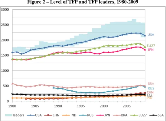
The fifth variable of interest is TFP. As already explained, TFP is endogenous in MaGE. It is determined by a catching up process in which distance to the technology frontier and education drive convergence. We add an exogenous gain or loss of TFP respectively in the high and low cases, but otherwise the process is kept unchanged. There will be a TFP gain as a result of additional technology transfer via FDI, exports (e.g. via contracts related to utilities, armament, power generation) or collaborative research. The TFP growth rate will increase with larger benefits for catching up countries with higher initial TFP growth rates. In contrast, in the low case, a deteriorating economic environment will produce the opposite evolution, which will be topped by capital destruction, and long term unemployment. Again the impact will be greater for catching up countries, and will have a detrimental effect on their growth rates. TFP shocks correspond to previously observed episodes. Figure 2 shows that, during the past 30 years, there have been many periods and many countries when TFP growth has slowed or become negative, or alternatively experienced buoyancy. The most notable include the transition of Russia after the fall of the USSR, and Japan during the 1990s. Our scenarios try to consider the impact of similar prolonged phases that are not captured by econometric estimation. The mechanisms described above (FDI, technology transfer, collaborative research) are topped by an overall technological boost in the high case, leading to a 50% increase in TFP for middle- and

6 _{Half-life time is defined as the time necessary to reduce by half the distance to the education frontier, assuming a}

19

income countries, and a 25% increase for high income economies only. Everyone is better off, but the technological leadership of high-income countries is eroded. The low case reflects ‘hard times’ when limited TFP gains in the North (just three-quarter of the gains projected in the reference scenario) lead to lower levels of technology transfer and tensions over intellectual property rights among this group of countries. As a result, TFP gains are even more reduced (-50%) in the group of catching-up countries. This is a less cooperative world in which everyone is worse off, but where the richest countries preserve part of their initial advantage.

Figure 2 – Level of TFP and TFP leaders, 1980-2009

Notes: TFP level is corrected for oil rents bias. Leader countries each year are the 5 countries with highest TFP, excluding Luxemburg. These countries include the USA, Denmark, Sweden, Ireland, Belgium, France, the Netherlands and Germany, depending on the year considered.

Source: MaGE, authors’ calculation.

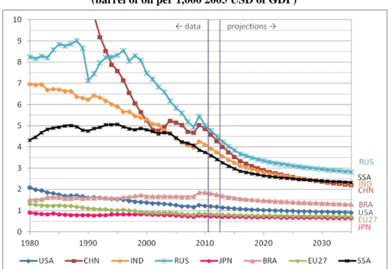
Another variable of interest is national energy efficiency. Technological breakthroughs could have a major impact on energy efficiency, since sectoral transition to less energy-intensive activities is endogenous, monitored by the conditionality of catching-up in energy productivity to GDP per capita, as depicted in Figure 3 for the MaGE reference case.7Here, we assume that countries at different levels of development will benefit unevenly from this progression. In the low case, technical progress occurs in the high income countries, but is not passed on to the middle- and low-income ones. Efficiency gains in energy accordingly are concentrated in the already most efficient countries (we assume a 50% increase with respect to the reference scenario), with lower impact on the overall energy efficiency of the world economy. In the high case efficiency gains are concentrated in the middle- and low-income countries, based on the assumption of increased transfers of the existing technology.

7 _{At the beginning of projections, almost every country had passed the turning point between efficiency decrease and}

20

Figure 3 – Energy intensity of the GDP in the reference scenario of MaGE, 1980-2035 (barrel of oil per 1,000 2005 USD of GDP)

Source: MaGE, authors’ calculation.

Figure 4 – Saving-Investment balance in the reference scenario, 1980-2035 (percentage of GDP)

21

Finally, capital mobility is an important determinant of growth since it shapes the difference between national saving and investment. Increased capital mobility should allow better allocation of capital worldwide and, thus, enhance growth overall. In the high case, we align the correlation between domestic saving and investment at world level with the lowest regional level, which is the one of the non-OECD countries. Note that this choice leads to no gain in capital mobility for the latter group of countries. However, in the low case, there is ‘financial de-globalization’, meaning that countries return progressively to financial autarky by 2050 (beyond the horizon of this exercise: thus, not achieved at the 2035 horizon).

Notice that assumptions about demographic profiles and capital mobility will modify the dynamics of the saving-investment balance depicted in Figure 4, characterized by a natural rebalancing of the Chinese economy.

The next step is to use the results of these two scenarios imposed on MaGE as inputs for MIRAGE. This provides two baselines that will experience additional shocks to the variables not included in MaGE (e.g. sectoral value added) and will become ‘High Sim’ and ‘Low sim’. For each scenario we compute the baseline scenario in MIRAGE on which we impose GDP, population, total labour force, skill level, saving, energy productivity, agricultural productivity, current account and energy price. We reproduce global trends in transaction costs consistent with the observed income elasticity of international trade (as already discussed) and recover TFP. As the energy price is exogenous, natural resources adjust endogenously at the baseline. Our two baselines assume status quo for tariffs as well as non-tariff barriers. We ultimately establish high and low for MIRAGE, which we call ‘High Ref’ and ‘Low Ref’ respectively (Table 5).

Table 5 – The two baselines of MIRAGE-e (2035 horizon)

Low Ref High Ref

MaGE scenario Low High

Energy prices High price Low price scenario

Transaction costs for goods* 25% cut 25% cut

Transports TFP* 2% annual growth 2% annual growth

Tariffs No change wrt 2007 No change wrt 2007

*

As discussed in the text, these two trends were introduced in a pre-experiment in order to reproduce long-term income elasticity of world trade.

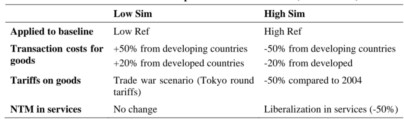
The final step consists of implementing trade scenarios in each of the two baselines (tariffs, transaction costs and NTM in services) with GDP and energy price set to be endogenous (TFP and natural resources fixed at their baseline level). These scenarios are summarized in Table 6. In the ‘Low sim’ scenario an increase in transaction costs and tariff is applied to the low baseline. The ‘High sim’ scenario starts from a high baseline and describes a more cooperative world where the barriers to trade in goods and services are reduced compared to their 2007 level.

In the ‘Low Sim’ scenario, we impose on the ‘Low Ref’ baseline a series of shocks reproducing an increase in transaction costs and a tariff war. In the context of a low growth profile and, possibly, geopolitical tensions, countries increase bureaucracy at the border, and systematize container scanning. Developing countries are more affected by this since their exports are perceived as ‘unsafe’ by the advanced economies. This degradation of the world trading environment is progressive: we add a 20% increase in the transaction costs for developed countries’ exports, linearly over the period considered (2014-2035). The increase peaks at 50% for developing countries’ exports. The second dimension to this degradation of the trading environment refers to protectionism. Countries either

22

respect de jure WTO commitments and rely almost exclusively on anti-dumping duties and safeguards, or revert to using their bound tariffs, or contribute to the non-cooperative scenario in which earlier commitments cease to be respected. To reproduce this outcome, we assume a progressive return of the world economy to post-Tokyo Round levels of protection, over the two decades considered. This is implemented as follows.

Table 6 – The two scenarios implemented in MIRAGE-e (2035 horizon)

Low Sim High Sim

Applied to baseline Low Ref High Ref

Transaction costs for goods

+50% from developing countries +20% from developed countries

-50% from developing countries -20% from developed

Tariffs on goods Trade war scenario (Tokyo round tariffs)

-50% compared to 2004

NTM in services No change Liberalization in services (-50%)

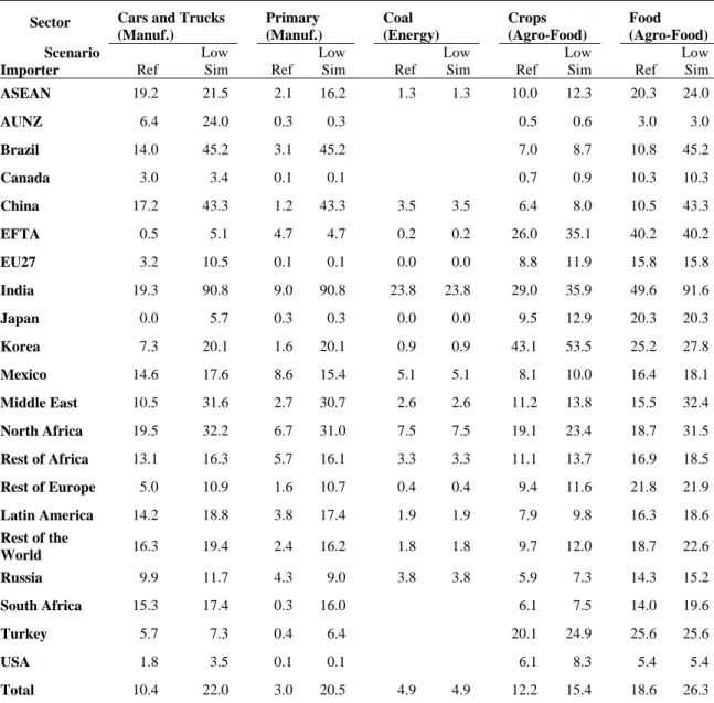
For manufacturing, we try to reproduce post-Tokyo Round tariffs. We use available data from Deardorff and Stern (1983) by sector. For aggregated regions, we adopt a simple average. For the rest, we take the oldest data from the World Development Indicators (WDI) to which we add a 25% increase. For the agro-food sector, we simply reverse the Uruguay round (Agreement on Agriculture) and add 36% to developed countries’ tariffs and 24% to those of developing countries; for energy goods, we keep tariffs constant. Tariffs within Free Trade Areas (FTAs) are assumed not to be subject to a tariff war and are not increased in our scenario. This affects the EU27, EFTA, NAFTA, AU-NZ and USA-AUNZ. These tariff increases provide a target for 2030, which we implement linearly between 2013 and 2030. Tariffs are constant after 2030. We present this procedure in Table 7 for selected sectors.8

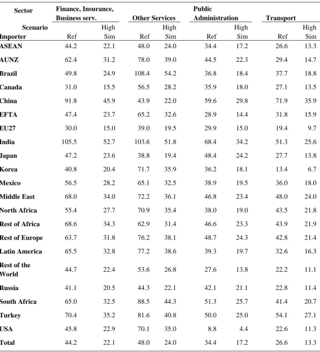
The high scenario (‘High sim’) describes a more cooperative world. Firstly, tariffs on goods are reduced (-50%) compared to their 2007 level. Secondly, benefiting from sustained growth and rapid convergence of emerging countries (increasing income levels and reducing costs of competition), countries address the issue of trade in services. There is a large decrease in the barriers to trade in services, and transaction costs on goods continue to decrease and decrease faster for developing countries where progress margins are bigger. We assume a 50% decrease in transaction costs for developing countries and a 20% decrease for developed countries.9 Regarding the reduction in the barriers to trade in services, we start with the ad valorem equivalents computed by Fontagné et al. (2011), modeled here as a trade cost. We then set the target to -50% in 2030, and this phasing out is implemented linearly between 2013 and 2030. The outcome of this exercise is shown in Table 8. Finally, the overall three-step method is summarized in Figure 5.

8 _{This methodology implies that targeted tariffs may be lower than or equal to the 2004 tariff in GTAP. For primary}

products, tariffs are not available in Deardorff and Stern and we use 2004 levels. For 252 triplets out of 9,261 this situation occurs as a result of averaging bias (sectors where the tariff decreased to less than the average value) or to aggregation bias (our simple average does not match the GTAP weighted average).

23

Table 7 – Tariff scenario by importer for selected sectors, ‘Low Sim’ versus ‘Ref’

Sector Cars and Trucks

(Manuf.) Primary (Manuf.) Coal (Energy) Crops (Agro-Food) Food (Agro-Food) Scenario Importer Ref Low Sim Ref Low Sim Ref Low Sim Ref Low Sim Ref Low Sim ASEAN 19.2 21.5 2.1 16.2 1.3 1.3 10.0 12.3 20.3 24.0 AUNZ 6.4 24.0 0.3 0.3 0.5 0.6 3.0 3.0 Brazil 14.0 45.2 3.1 45.2 7.0 8.7 10.8 45.2 Canada 3.0 3.4 0.1 0.1 0.7 0.9 10.3 10.3 China 17.2 43.3 1.2 43.3 3.5 3.5 6.4 8.0 10.5 43.3 EFTA 0.5 5.1 4.7 4.7 0.2 0.2 26.0 35.1 40.2 40.2 EU27 3.2 10.5 0.1 0.1 0.0 0.0 8.8 11.9 15.8 15.8 India 19.3 90.8 9.0 90.8 23.8 23.8 29.0 35.9 49.6 91.6 Japan 0.0 5.7 0.3 0.3 0.0 0.0 9.5 12.9 20.3 20.3 Korea 7.3 20.1 1.6 20.1 0.9 0.9 43.1 53.5 25.2 27.8 Mexico 14.6 17.6 8.6 15.4 5.1 5.1 8.1 10.0 16.4 18.1 Middle East 10.5 31.6 2.7 30.7 2.6 2.6 11.2 13.8 15.5 32.4 North Africa 19.5 32.2 6.7 31.0 7.5 7.5 19.1 23.4 18.7 31.5 Rest of Africa 13.1 16.3 5.7 16.1 3.3 3.3 11.1 13.7 16.9 18.5 Rest of Europe 5.0 10.9 1.6 10.7 0.4 0.4 9.4 11.6 21.8 21.9 Latin America 14.2 18.8 3.8 17.4 1.9 1.9 7.9 9.8 16.3 18.6 Rest of the World 16.3 19.4 2.4 16.2 1.8 1.8 9.7 12.0 18.7 22.6 Russia 9.9 11.7 4.3 9.0 3.8 3.8 5.9 7.3 14.3 15.2 South Africa 15.3 17.4 0.3 16.0 6.1 7.5 14.0 19.6 Turkey 5.7 7.3 0.4 6.4 20.1 24.9 25.6 25.6 USA 1.8 3.5 0.1 0.1 6.1 8.3 5.4 5.4 Total 10.4 22.0 3.0 20.5 4.9 4.9 12.2 15.4 18.6 26.3 Note: Simple average. ‘Ref’ is the baseline tariff used for ‘Low Ref’ and ‘High Ref’. ‘Low Sim’ is the

scenario value.

24

Table 8 – NTM tariff equivalent in services by importer

Sector Finance, Insurance,

Business serv. Other Services

Public Administration Transport Scenario Importer Ref High Sim Ref High Sim Ref High Sim Ref High Sim ASEAN 44.2 22.1 48.0 24.0 34.4 17.2 26.6 13.3 AUNZ 62.4 31.2 78.0 39.0 44.5 22.3 29.4 14.7 Brazil 49.8 24.9 108.4 54.2 36.8 18.4 37.7 18.8 Canada 31.0 15.5 56.5 28.2 35.9 18.0 27.1 13.5 China 91.8 45.9 43.9 22.0 59.6 29.8 71.9 35.9 EFTA 47.4 23.7 65.2 32.6 28.9 14.4 31.8 15.9 EU27 30.0 15.0 39.0 19.5 29.9 15.0 19.4 9.7 India 105.5 52.7 103.6 51.8 68.4 34.2 51.3 25.6 Japan 47.2 23.6 38.8 19.4 48.4 24.2 27.7 13.8 Korea 40.8 20.4 71.7 35.9 36.2 18.1 13.4 6.7 Mexico 56.5 28.2 65.1 32.5 38.9 19.5 36.0 18.0 Middle East 68.0 34.0 72.2 36.1 46.8 23.4 48.0 24.0 North Africa 55.4 27.7 70.9 35.4 38.0 19.0 43.5 21.8 Rest of Africa 68.6 34.3 62.9 31.4 46.6 23.3 43.9 21.9 Rest of Europe 63.7 31.8 76.2 38.1 48.7 24.3 42.8 21.4 Latin America 65.5 32.8 77.2 38.6 39.3 19.7 32.6 16.3 Rest of the World 44.7 22.4 53.6 26.8 27.6 13.8 22.2 11.1 Russia 41.1 20.5 44.3 22.1 42.1 21.1 22.8 11.4 South Africa 65.0 32.5 88.5 44.3 51.3 25.7 41.4 20.7 Turkey 70.4 35.2 81.6 40.8 50.0 25.0 54.1 27.1 USA 45.8 22.9 70.1 35.0 8.8 4.4 22.6 11.3 Total 44.2 22.1 48.0 24.0 34.4 17.2 26.6 13.3 Note: Simple average. Ref is the baseline level and ‘High Sim’ is the scenario values.

25