HAL Id: hal-01287838
https://hal.archives-ouvertes.fr/hal-01287838
Preprint submitted on 14 Mar 2016
HAL is a multi-disciplinary open access
archive for the deposit and dissemination of
sci-entific research documents, whether they are
pub-lished or not. The documents may come from
teaching and research institutions in France or
abroad, or from public or private research centers.
L’archive ouverte pluridisciplinaire HAL, est
destinée au dépôt et à la diffusion de documents
scientifiques de niveau recherche, publiés ou non,
émanant des établissements d’enseignement et de
recherche français ou étrangers, des laboratoires
publics ou privés.
Copyright
Power Modeling and Exploration of Dynamically
Reconfigurable Multicore Designs
Robin Bonamy, Sébastien Bilavarn, Daniel Chillet, Olivier Sentieys
To cite this version:
Robin Bonamy, Sébastien Bilavarn, Daniel Chillet, Olivier Sentieys. Power Modeling and Exploration
of Dynamically Reconfigurable Multicore Designs. 2013. �hal-01287838�
Power Modeling and Exploration of Dynamically
Reconfigurable Multicore Designs
R
OBIN
B
ONAMY1
, S
ÉBASTIEN
B
ILAVARN2,*
, D
ANIEL
C
HILLET1
,
AND
O
LIVIER
S
ENTIEYS1
1CAIRN, University of Rennes 1, CNRS, IRISA 2LEAT, University of Nice Sophia Antipolis, CNRS *Corresponding author: bilavarn (at) unice (dot) fr
This paper exhaustively explores the potential energy efficiency improvements of Dynamic and
Partial Reconfiguration (DPR) on the concrete implementation of a H.264/AVC video decoder.
The methodology used to explore the different implementations is presented and formalized.
This formalization is based on pragmatic power consumption models of all the tasks of the
application that are derived from real measurements. Results allow to identify low energy /
high performance mappings, and by extension, conditions at which partial reconfiguration can
achieve energy efficient application processing. The improvements are expected to be of
57%
(energy) and
37% (performance) over pure software execution, corresponding also to 16% energy
savings over static implementation of the same accelerators for
10% less performance.
1. INTRODUCTION
Minimizing power consumption and extending battery life are major concerns in popular consumer electronics like mobile handsets and wireless handheld devices. Silicon chips embed-ded in these products face challenging perspectives with the rise of processing heterogeneity introduced to address heat and power density problems. Efficient methodologies and tools are thus necessary to help the mapping and execution of applica-tions on such complex platforms considering high demands for performance at less energy costs.
In the context of mobile devices, the video decoding is known as part of intense computation, and this leads to important im-pact on energy consumption. Considering this context and the need of methodology to help the designers of such systems, it is essential that a subset of relevant solutions can be quickly identified and evaluated from early steps of development. This process usually relies on high level modeling and estimations to help analyzing many complex interactions between a variety of implementation choices. Performance models of FPGAs have been widely addressed but power consumption has been less investigated in comparison, especially regarding Dynamic and Partial Reconfiguration (DPR).
DPR is a feature introduced to further improve the flexibility of reconfigurable based hardware accelerators. It exploits the
ability to change the configuration of a portion of a FPGA while other parts are still running. By sharing the same area for the execution of different sequential tasks, DPR allows reducing the size of active programmable logic required for a given ap-plication, [1,2]. Therefore, improving the area efficiency also results in decreasing static power consumption which is directly linked to the number of transistors in the chip. The counterpart is that an additional part of power is needed to switch from a current configuration to the next one. Thus, this DPR cost needs to be properly assessed and analyzed in order to check if there is an actual power consumption benefit at the complete system level, for a given application. This paper investigates the exploitation of this on a relevant case study addressing the implementation of a H.264/AVC video decoder in search of the best global energy efficiency at the complete system level. From this concrete example, we define a pragmatic formalisation of the problem that can be used to analyze any mapping combina-tion of dynamic hardware and software tasks, and to provide reliable evaluations of execution time, area, power and energy. In particular, all components of power consumption, based on real implementation and power measurements, are considered to define the models and compute the estimations which include the overheads of task level DPR utilization. It is thus shown in the results how this can lead to verify more systematically the improvements of DPR and potential of partial reconfiguration
for energy efficient video processing. These results take into ac-count of the reconfigurable overhead in terms of performances and power consumption.
The paper firstly presents state of the art techniques in the field of DPR acceleration in Section 2, with a special emphasis on energy analysis and optimisation. Then Section 3 details formal models for application, platform and dynamic reconfiguration underlying the mapping analysis of the H.264/AVC decoder. The automatic analysis of different mappings and scheduling of hardware and software application tasks is described in Section 4. Then, a result analysis of the full video application deployment is presented along with estimation values that are discussed in Section 5. Finally, we conclude the paper and suggest future directions for research.
2. DYNAMIC PARTIAL RECONFIGURATION AND EN-ERGY EFFICIENCY
Embedded systems have to cope with numerous challenges such as limited power supply, space and heat dissipation. Extensive research efforts are currently carried out in order to address these problems. Reconfigurable architectures and FPGAs have been attractive in embedded systems due to their flexibility, allowing faster development at lower costs than Application Specific In-tegrated Circuits (ASICs). However, the energy efficiency and the maximum frequency of reconfigurable hardware are also impaired by their flexible interconnect do not allow to reach the power performance level of custom ASICs [3,4].
Dynamic and Partial Reconfiguration is a feature that became effective fairly recently and brings new opportunities to improve processing efficiency. Firstly, DPR allows a better use of hard-ware resources by sharing and reusing reconfigurable regions (PRRs) during execution, thus less area and energy consumption are expected. A variety of other techniques can be associated to this inherent DPR capability. For instance, it is possible to clear the configuration data of a PRR (referred to as blank con-figuration in the following) when it is unused which leads to decrease the share of static power associated with PRRs [5]. As an important part of power consumption also comes from clock signals, some techniques investigated the use of dynamic recon-figuration to reduce clock related impacts. A low overhead clock gating implementation based on dynamic reconfiguration has been proposed in [6], achieving 30 % power reductions com-pared to standard FPGA clock-gating techniques based on LUTs. Another approach has been developed to modify the parameters of clock tree routing at run time reconfiguration to moderate clock propagation in the whole FPGA and decrease dynamic power [7]. Finally, self-reconfiguration also permits online modi-fication of clock frequency with low resource overhead by acting directly on clock management units from the reconfiguration controller [8].
Dynamic and partial reconfiguration faces the difficult prob-lem of task placement, both spatially on reconfigurable regions and temporally in terms of scheduling. Therefore DPR demands specific requirements to support this type of execution. It is generally the responsibility of a task scheduler, like [9], to decide online which resource will support the execution of a task. The question becomes even more critical when addressing context saving issues related to the preemption and relocation of hard-ware tasks as discussed for example in [10]. In terms of power, scheduling must state when task reconfiguration occurs such as to avoid unnecessary idle consumption prior to execution [11]. It is also responsible for choosing to use blank configurations
or not while ensuring this decision actually leads to an overall energy gain [12].
Another important element in DPR optimization is related to hardware implementation and parallelism. Parallelism has the potential to decrease the execution time of an hardware im-plementation up to several orders of magnitude. A technique to exploit this potential is to apply code transformations such as those available in High Level Synthesis (HLS) tools. Previous works reported two times energy reductions between sequential and unrolled loops of a hardware matrix multiplication imple-mentation [13]. This parallelism exploitation is especially rel-evant for DPR since it can help the adaptation of a better area power performance tradeoff at run time.
However, all these opportunities add many dimensions to the DPR implementation problem for which there are currently few design analysis support, especially concerning energy and power consumption. It is thus extremely difficult to i) identify the most influential parameters in the design and ii) understand the impact of their variations in search of energy efficiency. In the following, we detail the deployment analysis of a H.264/AVC decoder on a representative performance execution platform (multicore with DPR), and in the most energy efficient way. To support this, we present first a formal model of application, platform and mapping to allow a more systematic exploration and evaluation of their associated impacts. Relevant power and energy models of DPR represent another essential condition to provide early reliable evaluations. The power and energy models that are used in the proposed exploration are based on actual measurements of the DPR process which are further described in [14]. Finally, a greedy exploration heuristic is made out of this base and described in details. It is shown in the result analysis how a set of relevant energy and performance tradeoffs can be identified and compared against characteristic solutions (best performance, static hardware, full software execution, etc.).
3. PROBLEM MODELING
Previous work addressed a detailed study of DPR energy mod-eling which led to identify significant parameters of dynamic reconfiguration (FPGA and PRRs idle power, DPR control) [14]. This section fully extends the model to support a full and realis-tic platform (hardware, software execution units), application (hardware, software tasks) and mapping characterization which is defined from a set of actual power values measured on real platforms reported in section Band C.
A. Target platform model
As previously stated, the target platform is a heterogeneous architecture that can be composed of processors and dynami-cally reconfigurable accelerators. Each type of execution unit is formalized by a set of specific parameters that captures all the information needed for deployment exploration. These parame-ters can be broadly classified in three categories that are listed in Table1: platform topology, execution units and dynamic and partial reconfiguration characterization.
A.1. Platform topology
Execution Units (EU) are divided in two categories: a number Ncoreof software execution units, processor cores, and NPRR hardware execution units, which are the partially reconfigurable regions of the FPGA. Therefore, the total number of hardware and software execution units NEUin the architecture is Ncore+ NPRR, and the jthexecution unit of the architecture is tagged
Table 1.Parameters used for heterogeneous architecture formalization Variable Range Definition Ncore ∈N∗
Number of software execution units NPRR ∈N∗ Number of hardware execution units NEU = NPRR+ Ncore Total number of execution units EUj ∀j = 1, ..., NEU The jthexecution unit
SoC = {EUj} A platform is a set of execution units
Njf req ∈N∗ Number of frequencies for software EU
j Fj,k ∀k = 1, ..., Njf req The kthfrequency of software EUj
Pemptyj,k ∈R+ Empty power consumption for software EU
jat Fj,k
Prun
j,k ∈R
+ Running power consumption for software EU
jat Fj,k
Ncell
j ∈N∗ Number of logic cells for hardware EUj Nbram
j ∈N
∗
Number of RAM blocks for hardware EUj Njdsp ∈N∗
Number of DSP blocks for hardware EUj
Pemptyj ∈R+ Empty power consumption for hardware EU
j
T1cell ∈R+ Time required to reconfigure one logic cell
E1cell ∈R+ Energy required to reconfigure one logic cell
by EUj with j ∈ [1, NEU]. In this abstract representation, a heterogeneous SoC platform is represented by the set of all its execution units{EUj}and this composition is considered fixed at run-time.
A.2. Execution units
The size of a hardware unit EUj is characterized in terms of logic resources with parameters Njcell, Njbramand Njdspto ensure realistic resource representation. The cell terminology refers to the main configurable resource of the programmable logic (e.g. Xilinx Slices, Altera Logic Elements).
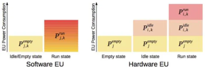
Concerning the power model, a distinction is made between different components of each EUj. The empty power consump-tion, Pjemptyor Pemptyj,k , reflects the power consumed when no application task is loaded, respectively for PRRs and cores (at frequency Fj,k). It is worth noting concerning PRRs that a task configured on it accumulates two contributions: Pi,kidlewhen the task is idle, and Pi,krunwhen it is running, which are both imple-mentation dependent and therefore described in the SectionB.3. The characterization of Pjemptyis additonally useful to consider PRR blanking opportunities in the analysis of task deployments. For software units, Pj,krunis the power of a core EUjrunning at Fj,k (full load). The energy of a software task can then be computed from Pj,krunand the corresponding execution time.
A.3. Dynamic and partial reconfiguration
Taking into account the cost of dynamic and partial reconfigura-tion involves two types of overhead: delay and energy. As the reconfiguration delay is mainly dependent on the speed of the re-configuration controller and size of the re-configuration bitstream, it can be efficiently described by parameter T1cellrepresenting the time needed to configure one logic cell and reflects the per-formance of the reconfiguration controller. Power is addressed in a similar way by parameter E1cellreflecting the energy needed to configure one logic cell. As configuration depends mostly on the number of logic cells composing a PRR in practice, delay and energy overheads are fairly easy to compute.
B. Application power and mapping model
Different features of the application tasks need to be known for exploration and estimation. These characteristics are formalized by a set of parameters that are exposed in Table2and that can be classified in three categories: task graph, task implementations and task execution characterization.
B.1. Task graph
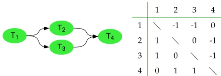
A task-dependency graphGis used to reflect execution concur-rency in the mapping problem. The dependencies between tasks are enumerated by an adjacency matrix representation which is convenient to process by an analysis algorithm. The adjacency matrix is a NT×NTmatrix used to represent dependencies be-tween tasks. Considering a row i, the value in each column is 1 if Tiis dependent on the task represented by the column index, otherwise this value is 0. This adjacency matrix is asymmetric and -1 values are used to represent an inverted edge direction of the graph (Figure 1). In addition, the adjacency matrix is completed with another information called the task equivalence matrix Ti1,i2eq , which is used to indicate the identicalness of two or more tasks, meaning that they have the same execution code or bitstream. This is useful to minimize execution units and improve their utilization rate, which is an important condition for DPR efficiency as it will be pointed out in the results.
T1 T2 T3 T4 1 2 3 4 1 -1 -1 0 2 1 0 -1 3 1 0 -1 4 0 1 1
Fig. 1.Simple graph task example and it’s associated adja-cency matrix.
B.2. Task implementations
From previous representation, it is also required to describe the possible implementations for each task. As we aim to explore
Table 2.Parameters used for application formalization
Variable Range Definition
NT ∈N∗ Number of tasks of the application Ti ∀i = 1, ..., NT The ithtask of the application G = {Ti} Task-dependency graph
Ti1,i2eq ∈ {0, 1} ∀i1, i2 = 1, ..., NT Tasks equivalence matrix
Niimp ∈N∗ Number of implementations of T i Ti,k ∀k = 1, ..., Niimp The kthimplementation of Ti
Ii,j,k ∈ {0, 1} Defines if Ti,kis instantiable on EUj
Ci,j,k ∈R+ Execution time of Ti,k
Ei,j,k ∈R+ Energy consumption of Ti,kon EUj
Pidle
i,k ∈R+ Idle power consumption of Ti,k Prun
i,k ∈R+ Running power consumption of Ti,k
combinations of mappings to the execution units, various imple-mentations of the same task can be described. Different software (CPU core, frequency) and hardware (PRR) implementations can be specified to reflect several power performance tradeoffs in the exploration. The total number of possible hardware and software implementations for task Tiis Niimp, and Ti,kis used to represent the kthimplementation of task Tiwith k∈ [1, N
imp i ].
B.3. Task execution
First, a variable Ii,j,kis used to express if Ti,kcan be executed using EUj(0 false, 1 true). When task Tiis running on a software execution unit (EUjat frequency Fj,k), the corresponding exe-cution time and energy consumption are defined by Ci,j,kand Ei,j,k. Energy can be derived from the power characterization of a CPU core: Ei,j,k=Pj,krun∗Ci,j,k.
Fig. 2.Power contributions of an execution unit.
A slightly different model applies for hardware tasks (Figure 2). When the kthimplementation of a hardware task is mapped to a PRR, it comes with a part of idle power. This contribution is referenced by Pi,kidlefor the kthimplementation of task Ti. The remaining power contribution Pi,krunis added when the task is running. Therefore, the total power of PRR EUj when Ti,kis configured and running is Pi,kidle+Pjempty+Pi,krun.
C. Model assesment
We apply previous modeling on the H.264 decoder in a way to evaluate the extent of the formalization defined and show the actual setting of model parameters from a clear measure-ment process. This characterization example is based on a dual CortexA8/Virtex-6 LX240T potential platform. Further details of the specification graph and functions of the video decoder are given in Section5.
C.1. Power measurement procedure
The FPGA device which is addressed in the following of this study is a Xilinx Virtex-6 LX240T. All measurements to set up the different parameters of the models are thus made on a Xilinx ML605 platform, including a built-in shunt resistor that can let us monitor the current through the FPGA core.
1V VC C I N T Shunt 5m
Virtex-6
Vcore GND + -×100 ML605Fig. 3.Current measurement schematics on ML605 Board using a high-precision amplifier.
Figure3shows the experimental setup for power measure-ments. We use the Virtex core shunt with a high-precision ampli-fier to handle current and power measurements that are logged with a digital oscilloscope. This setup allows to measure dy-namic variations of current and power consumptions as low as milliamps and milliwatts during the execution of the device.
C.2. Platform
A first issue is to determine a set of relevant PRRs in terms of number (NPRR) and size (Njcell, Njbram, Njdsp). We do not handle this partitioning in our approach and rely on the methodology of [15] which defines a systematic approach to achieve this. Then, the empty power of PRRs (Pjempty) can be derived from the empty power per logic cell, which is the power that can be measured when the full FPGA is powered but does not contain any config-uration (at voltage and internal temperature constant), averaged by the number of cells. For instance, the Virtex-6 device used has a measured empty power of 1.57W (at 1V, 35°C) for a capability of 37680 slices, which leads to a parameter of 41.7 µW/slice. It is then easy to derive the empty power of a PRR from its size. The configuration of a task on a PRR also adds contributions that are implementation dependent (Pidlej,k , Pruni,k ), the determination of these parameters is thus described in the following section.
Empty and running power of CPU cores come from similar measurements. It is worth noting here that the model let the specification of different types of cores and frequencies (Fj,k). A
software implementation can be associated to a core frequency k in this case. Pj,kemptyand Pj,krunare the consumptions measured respectively when the core is idle (no application task) and run-ning (assuming 100% CPU load). As an illustration, these values are 24mW and 445mW for an OMAP3530 based platform operat-ing at 600MHz [16].
The power model used for DPR reconfiguration is the Coarse Grained DPR estimation model detailed in [14]. In the example of SectionB, this model is calibrated for an optimized recon-figuration controller called UPaRC [17] supporting 400 MB/s at an average power of 150 mW. The minimum reconfig-uration region in a Virtex-6 device (one cell = one slice) is one frame, where one frame is 324 bytes and contains two slices [18]. In these conditions, the corresponding T1cell is
(324B / 400MB/s)/ 2=0.41 µs. In addition, the related E1cell is T1cell×150 mW=61.5 nJ. From these values, it is convenient to derive reconfiguration delay and energy for PRRs of different shapes and sizes.
C.3. Application
In the formalism of Table2, hardware and software task map-ping parameters can be settled by defined implementations and measures. Classical profiling can be used to set out software execution time Ci,j,kand derive the associated energy cost Ei,j,k from the power Pj,krunof the executing core at frequency k (e.g. E1,1,1=445mW∗5ms=2.23mJ for T1on core EU1in Table5).
As for hardware tasks, they are fully generated using an ESL (Electronic System Level) methodology described in [19]. Hardware mapping parameters are derived from measurements made possible by full accelerator implementation. Pi,kidleis the consumption measured when Ti,kis configured but not running. This power is supposed to be independent from PRRs in our model. Pruni,k is the fraction of dynamic power added when Ti,k is running (also supposed independent from PRRs), that can be determined in practice by subtracting the consumption of a configuration where Ti,kis running from the consumption of a configuration where Ti,kis idle. Therefore, the total power of a hardware task Tiis the sum of P
empty
j of a PRR and Pi,kidlewhen the task is idle, plus an additional contribution Pi,krunwhen the task is running. For example, the first hardware implementation I5,4,2of T5,2 on EU4(PRR2) in Table5has a total energy cost E5,4,2computed from P
empty
4 of PRR2, P5,2idle/P5,2runof T5,2, and the corresponding execution time C5,4,2:
E5,4,2 = (P4empty+P5,2idle+P5,2run) ∗C5,4,2
= (137mW+34.2mW+11.47mW) ∗2.46ms
= 0.45mJ.
This view is actually integrated in a more global framework for power modeling and analysis called Open-PEOPLE [20]. In particular, the open power platform supports remote measure-ments and therefore let the definition of previous parameters reducing the need for equipment, devices and the usually com-plex monitoring procedures associated. The following section shows how using previous models developed from a set of acu-rate and concrete measurements can help defining relevant and reliable deployment exploration analysis.
4. DEPLOYMENT ANALYSIS
Based on previous modeling and formalization, more method-ological approaches can be defined to explore the mapping space and provide relevant evaluations. Execution time, area (in terms
of programmable logic resources), energy and power profiles can be computed from the full characterization of the system available, including description and power models of execution units, SoC platform, Hw/Sw implementations of tasks, Dynamic Partial Reconfiguration and Partial Reconfigurable Regions. Fig-ure4depicts the exploration methodology used for this energy efficiency study, and is further detailed in the following.
A. Exploration inputs
A.1. System description
The estimation flow starts with descriptions of application tasks and execution resources (Figure 4-1-). Tasks dependencies are specified using the aforementioned task-dependency graph (G, NT, T
i, Ti1,i2eq ), which is further processed using graph traversal techniques. Platform resource information like the size, number of PRRs and CPUs must be considered to determine different possible allocations. We assume here that the definitions of PRRs have been done so far (SectionC.2). Hw/Sw implementations of tasks and SoC platform characteristics required to compute power estimations come from specific libraries that are described in the following.
A.2. SoC libraries
Power consumption and execution time of tasks for each possi-ble execution unit are described in Tasks Implementation libraries (Figure 4-2-). For hardware tasks, these settings can be esti-mated by hardware dedicated power estimators, like the Xilinx Power Estimator [? ], and execution time can be derived from timing reports produced by high level synthesis. Energy of soft-ware tasks can also be based on measurements or derived from data released by processor manufacturers. However for the sake of precision, power and execution times in the following come from real implementation and measurement for both hardware and software tasks (SectionC.3).
Specific power and energy models are used to estimate the overheads resulting from PRR reconfigurations. These mod-els have enough accuracy to estimate the latency, energy, and power profile of a reconfiguration from the characteristics of the reconfiguration controller, PRR and tasks involved [14].
Another aspect in the estimation model is the power con-sumed by a hardware task present on a PRR, but not in use (idle power). An idle task power model is used to compute this contri-bution from sizes of tasks and PRRs. An improvement here is to configure a PRR with an empty task to reduce the associated idle power. This possibility is included in the mapping exploration process (Figure 4-8-).
Finally, device parameters such as the size, process technol-ogy and external adjustments like voltage and frequency are also present in SoC Parameters. This type of information is not currently used in the computation of estimations. Since previous libraries have been derived from measurements on a specific device (Virtex-6), we kept these characteristics in a way to derive implementations and models for different technologies.
B. Ordered execution lists
Scheduling and allocation must be known in order to compute performance and energy estimations. We use information de-rived from the task-dependency graph to define a preliminary order for the execution of tasks. This is the role of the Ordered Execution List (OEL), which is a list of tasks similar to the task graph except that it sequentially determines which tasks must be launched for a time slot (τn). Each time slot corresponds to the end of a task and the beginning to, at least, one other task. The
Ordered Execution List System description Hardware Implementation Software Implementation Results SoC librairies HW/SW mapping Dynamic Partial Reconfiguration Cost
time + energy cost
Execution Cost
time + energy + resource cost
Auxiliary power drain
- Hardware idle tasks - Static power - Idle power
Partial Reconfiguration Model
- bitstream size
- reconfiguration controller energy efficiency - reconfiguration controller performance
Resources -CPUs -PRRs Application -Tasks -Task-dependency graph -Tasks equivalence
Idle Tasks Power Model Blanking ?
yes
Dynamic Partial
Reconfiguration Cost
time + energy cost
Exhaustiveenergy time and area
exploration
Most energy efficient HW/SW execution order
and implementation
Fastest execution time HW/SW execution order and implementation Configuration required? Hardware yes no Software no Exp_Golomb MB_Header Inv_CAVLC Inv_Pred Inv_QTr DB_Filter Execution Cost time + energy + resource cost
SoC power model
-static -IO -CPU idle -clock tree SoC Parameters - technology - frequency - supply voltage Execution time E ne rg y Area Implementation Exploration NcoreNPRRNEUSoC NT Ti Ti1 ,i2 eq Mapi , j , k ,τn T1slice E1slice Pi, k idle Pj empty Nj cell Nj BRAM Nj DSP
1
2
3
4
5
6
7
8
9
Tasks Implementation librairies Ni imp Ci , k Ei, k Ii, j , k G τn=1 τn=2 τn=3 τn=4 τn=5Fig. 4.Global exploration and power / performance estimation flow.
Table 3. OEL parameters used in exploration
Variable Range Definition
NOEL ∈N∗ Number of OELs extracted from G NTS
n ∀n = 1, ..., NOEL Number of time slots in the nthOEL
τn = 1, ..., NnTS Current time slot of the nthOEL OELτn ,i ∈ {0, 1} Presence of Tifor τn
OEL is a representation of a static task schedule which is useful to derive at low complexity a number of feasible deployments. This ensures keeping enough workstation capacity to process the analysis of extensive task mappings along with fine complete power characterizations.
However, one OEL is not always enough to cover the best scheduling solution, especially if the application supports a lot of parallel tasks. An example is shown in Figure4-3- where tasks Inv_Pred and Inv_QTr are executed in the same time slot, whereas Inv_Pred could also be run in parallel with Inv_CAVLC. In such a case, several OELs can be extracted fromGand explored one by one. The mapping definition process from an OEL depends on the formal parameters of Table3and is further described in the next section.
C. Mapping exploration
C.1. Implementation selection
For each task beginning at the current time slot τn, an imple-mentation is selected from the list of possibilities (hardware or software) available in the task implementation library (Figure4 -4-). Mapk,i,j,τnis a variable which represents the implementation
choice by its value: 1 at τnwhen Ti,kis mapped on EUj. This variable is also set under the following constraints:
- one task is mapped only once
∑
j,k,τn
Mapk,i,j,τn =1 ∀i∈1, ..., NT (1)
- one EU can run only one task at the same time
∑
i,k
Mapk,i,j,τn ≤1 (2)
∀j∈1, ..., NEU, ∀τn∈1, ..., NnTS
For a mapping choice expressed by Map, estimations of power and execution time are then computed subsequently.
C.2. Partial reconfiguration cost
Reconfiguration is likely to occur when a task is mapped on a hardware execution unit (PRR), except if this task is already configured on this PRR (Figure4-5-). In the situation where a re-configuration is needed (Figure4-6-), time and energy overheads are computed respectively by:
Tjcon f = T1cell×Njcell (3)
Econ fj = E1cell×Njcell (4)
C.3. Task execution cost
Contributions of the actual execution of tasks (hardware and software) are then added to previous cost estimation (Figure 4-7-). The execution time for the current implementation of task Tiis given by Ci,j,kwhile the energy consumption for this implementation is defined by Ei,j,k.
C.4. Blanking analysis
When a hardware resource is not used for some time, blanking is an opportunity that can also be considered to save power (Figure 4-8-). However this technique comes with an added cost that has to be estimated [12]. This is determined by comparing the energy with and without blanking using the following expressions:
Eblankingj = Econ fj +Eemptyj
= Econ fj +Pjempty∗ (Tjidle−Tjcon f) (5)
Ei,j,kidle = Pi,kidle∗Tjidle (6)
where Tjidleis the time during which EUjis idle, waiting for a new task to begin. If Eblankingj < Eidlei,j,kthen blanking is an acceptable solution.
D. Auxiliary power drain
Auxiliary power contributions are also considered to fully char-acterize the energy consumption (Figure4-9-). These contribu-tions are from the static leakage power and from the idle power of the clock tree, both considered in PSoCidle. The portion of power consumed by the execution units even when they are not in use (Pj,kempty) is also added. We consider that power of a blank PRR is included in Pjempty. However, hardware tasks already configured and idle also lead to power drains that are considered (Pidle
i,k )
E. Global cost characterization
At the end of an OEL analysis, energy contributions and exe-cution times are added for each global mapping solution. An exhaustive search is currently used to enumerate the possible de-ployments of tasks on the execution units. This process consists in generating progressively at each time slot different branches for the OEL mapping. The end of a branch corresponds to a global deployment solution with its associated estimation of en-ergy, area (resources) and performance. Notable solutions mini-mizing energy or performance are highlighted from a scatter plot representation of the results to help comparing the mappings explored (Figure6). Scheduling and the corresponding power profiles are computed as well to further analyze and implement a particular solution, as illustrated in Figure8. Next section outlines these results that are derived from the application to a parallelized accelerated H.264/AVC decoder.
5. APPLICATION STUDY AND RESULTS
As specified in the introduction section, the objective of this paper is to verify if the DPR can improve the execution perfor-mance (time, power and energy consumption) of the H.264/AVC video decoder. This section presents the results obtained for the exploration and show the different interesting mappings that can be chosen by the designer to satisfy the design constraints.
This section first presents the application model, then the platform used to explore the mapping and finally the results of the exploration.
A. H.264/AVC decoder
The application which is considered in this validation study is a H.264/AVC profile video decoder specification modified to comply with parallel software (multicore) / hardware (reconfig-urable) execution. An ESL design methodology [19] is used to provide real implementations for the possible hardware func-tions, which serve as an entry point to the exploration flow of Section4. The input specification code used is a version derived from the ITU-T reference code [? ] to better cope with hardware design constraints.
The deblocking filter (DB_Filter), inverse CAVLC (Inv_CAVLC), and inverse quantization and transform block (Inv_QTr) contribute together to 76% of the global execution time on a single CPU core. They represent the three functionalities of the decoder that can be either software or hardware executed.
Fig. 5.H.264 decoder task flow graph.
In addition to these acceleration opportunities, we aim at ex-ploring solutions mapped onto parallel architectures including multicore CPUs. For this, we consider a multithreaded version of the decoder exploiting the possibility of slice decomposition of frames supported in the H.264/AVC standard. Indeed a slice represents an independent zone of a frame, it can reference other slices of previous frames for decoding; therefore decoding one slice (of a frame) is independent from another (slice of the same frame). This way, the decoder can process different slices of a frame in parallel. We have thus considered a decomposition of the image where two streams process two halves of a same frame (Figure5). The corresponding task graph is defined byG
as:
G = {Exp_Golomb, MB_Header, Inv_CAVLC1, Inv_CAVLC2, Inv_QTr1, Inv_QTr2, Inv_Pred1, Inv_Pred2, DB_Filter1, DB_Filter2}. (7) This graph can be deployed using up to six accelerators and two processors on the underlying platform. Accelerators are fully generated from a reference C code at this level in a way to derive precise performance, resource, and power information, and to define relevant reconfigurable regions for DPR execution (Table4). Some functions are reported with two implementa-tions (sequential and parallel resulting from HLS loop unrolling) to account for the impacts of parallelism on energy efficiency. Software tasks are characterized in a similar way by running the code on CPU cores to derive execution times and energy, possibly at the different supported frequencies (Table5).
B. Target platform
The execution platform is based on two ARM CortexA8 cores and an eFPGA, assuming a Virtex-6 device model supporting DPR. Table4shows the corresponding platform parameters that have been set as exposed in SectionC.2. The method of [15] is used to identify an optimal set of PRRs under performance and FPGA layout constraints, considering all the hardware imple-mentations of tasks previously considered. Three PRRs of 1200, 3280 and 2000 slices were found to reduce slice and BRAM count from respectively 49% and 33% over a purely static implementa-tion of all hardware tasks. Therefore this configuraimplementa-tion is used as a basic PRR setup in the following deployment analysis.
From PV6LX240Tempty = 41.7 µW/slice measured previously on the device, it is possible to derive the empty power consumption
for each defined PRR: P3empty=50 mW, P4empty=137 mW and P5empty =83 mW. The empty power of CPU cores come from similar measurements on an OMAP3530 based development board: Pj,kempty=24 mW and Pj,krun=445 mW for a CortexA8 core at Fj,k=600MHz.
Additionally, the reconfiguration controller used is an opti-mized IP called UPaRC supporting a reconfiguration speed of 400 MB/s for a power of Pcontroller = 150 mW [17]. This cor-responds to T1cell = 0.41µs and E1cell = 61.5mJ (SectionC.2) from which reconfiguration time and energy of a PRR are easy to compute.
C. Application model parameters
Table5shows the application model parameters in details for the H.264 decoder example. The decoder is composed of ten tasks among which six can be run in hardware. All tasks are characterized in terms of software and hardware mapping fol-lowing the generation and measurement procedure of Section C.3.
For each hardware task (T5, T6, T9, T10), two versions of dif-ferent cost and performance tradeoffs are produced using HLS loop level parallelism. Therefore, if we consider the example of Inv_QTr1(T5), three implementations T5,1, T5,2, T5,3are possible with respectively 5.10ms (CortexA8 600MHz), 2.46 ms (hard-ware #1) and 1.97 ms (hard(hard-ware #2 with loop unrolling). For each of the two hardware implementations, three possible PRR mappings are described along with the associated energy cost (computed as shown inC.3). This realistic characterization of different task implementations based on practical data improves the reliability of estimations and exploration results, which are addressed in the following.
D. Exploration results and analysis
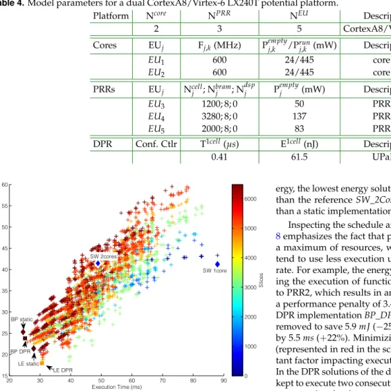
Under previous conditions of application, SoC architecture and dynamic reconfiguration, the primary output of the exploration flow is plotted in Figure6. It is worth noting first the very im-portant quantity of solutions analyzed, over 1 million possible mappings are evaluated for this design. This exploration ex-ample is processed in a matter of seconds with an Intel Core i5 based workstation.
Six solutions are highlighted from the results: (i) full soft-ware implementation using one CPU core (SW_1Core), (ii) full
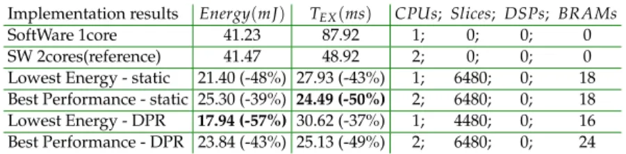
Table 4.Model parameters for a dual CortexA8/Virtex-6 LX240T potential platform.
Platform Ncore NPRR NEU Description
2 3 5 CortexA8/V6LX240T Cores EUj Fj,k(MHz) P empty j,k /Prunj,k (mW) Description EU1 600 24/445 core #1 EU2 600 24/445 core #2 PRRs EUj Ncellj ; Nbramj ; N dsp j P empty j (mW) Description EU3 1200; 8; 0 50 PRR #1 EU4 3280; 8; 0 137 PRR #2 EU5 2000; 8; 0 83 PRR #3
DPR Conf. Ctlr T1cell(µs) E1cell(nJ) Description
0.41 61.5 UPaRC 20 30 40 50 60 70 80 90 15 20 25 30 35 40 45 50 55 60 Execution Time (ms) E nerg y (mJ) SW 1core SW 2cores LE static BP static BP DPR LE DPR S lic es 0 1000 2000 3000 4000 5000 6000
Fig. 6.Energy vs. execution time exploration results. Colors represent the number of FPGA resources (slices) of a solution.
software execution using two cores (SW_2Cores), (iii) the low-est energy solution using static accelerators (LE_Static), (iv) the best performance solution using static accelerators (BP_Static), (v) the lowest energy solution using dynamic reconfiguration (LE_DPR) and (vi) the best performance solution using dynamic reconfiguration (BP_DPR). Details of these characteristic solu-tions are summarized in table 6. Since SW_1Core is almost twice slower for the same energy compared to SW_2Cores, SW_2Cores is considered as a reference result in the following to let the comparison of relative improvements from hardware acceler-ated solutions. To further help this analysis, exploration results also output scheduling, allocation and power profiles that are illustrated in figures 7and 8for BP_Static, LE_Static, BP_DPR and LE_DPR.
We can firstly note that the four accelerated solutions per-form better compared to the reference software execution, both in terms of performance and energy. Hardware significantly im-proves processing efficiency while offloading CPU cores which results in 50% faster execution and 39% energy savings at the global decoder application level. Dynamic reconfiguration in-troduces a slight performance penalty due to reconfiguration delays, however the best performance solution based on DPR is only 2.6% slower than a static implementation. In terms of
en-ergy, the lowest energy solution using DPR is 57% more efficient than the reference SW_2Cores and 16% more energy efficient than a static implementation.
Inspecting the schedule and resources usage of figures 7and 8emphasizes the fact that performance solutions make use of a maximum of resources, while low energy implementations tend to use less execution units and improve their utilization rate. For example, the energy of BP_Static is reduced by offload-ing the execution of function CAVLC from the first CPU core to PRR2, which results in an energy gain of 3.9 mJ (−15%) for a performance penalty of 3.4 ms (+14%). The same applies for DPR implementation BP_DPR in which Core1 and PRR3 can be removed to save 5.9 mJ (−25%) while increasing execution time by 5.5 ms (+22%). Minimizing the number of reconfigurations (represented in red in the scheduling profiles) is also an impor-tant factor impacting execution time and energy consumption. In the DPR solutions of the decoder, the configuration of PRR2 is kept to execute two consecutive instances of Inv_CAVLC, and the same applies for the execution of DB_Filter on PRR1. However, Inv_QTr is mapped to PRR1 for the first instance and to PRR2 for the second. Execution dependencies between DB_Filter and Inv_QTr do not allow to save a reconfiguration of Inv_QTr with-out a penalty on global execution time, impacting also energy. The second instance of Inv_QTr is thus executed on PRR2.
In terms of DPR benefits over static implementation, the H.264 decoder example shows that DPR brings 16% energy improvement for 31% FPGA resource (slice) reduction and an execution time increase of 10%. Energy gains come from the reduction of the static area of the programmable logic and the associated idle power, decreasing from 318 mW to 210 mW (34%). These results help evaluating the practical benefits of dynamic reconfiguration, considering also that there is room for improve-ment on the H.264 decoder by moving more functions to hard-ware.
Finally, it is also interesting to note that for this application, none of the four hardware solutions highlighted exploits PRR blanking. In the LE_DPR solution, hardware execution units are not free for a sufficient period of time to compensate the energy overheads implied by PRR reconfigurations. Therefore these estimations provide a possible assessment to know whether or not to use blanking in a design.
The end result from a potential platform made of two CPUs and a FPGA fabric is a solution based on a single core execu-tion with dynamic reconfiguraexecu-tion of six hardware accelerated functions on two PRRs. The corresponding implementation rep-resents 57% and 37% performance and energy improvements
Table 5.Task parameters for an H.264/AVC decoder application.
Ti Ti,k Ii,j,k=1 Ci,j,k(ms) Ei,j,k(mJ) Pidlei,k /Pruni,k (mW) Ncelli,k; Nbrami,k ; N dsp i,k Description T1 T1,1 I1,1,1I1,2,1 5.00 2.23 24/445 – Exp_Golomb T2 T2,1 I2,1,1I2,2,1 4.92 2.19 24/445 – MB_Header T3 T3,1 I3,1,1I3,2,1 11.03 4.91 24/445 – Inv_CAVLC1 T3,2 I3,4,2 7.45 1.46 55.1/4.4 3118; 6; 0 T4 T4,1 I4,1,1I4,2,1 11.03 4.91 24/445 – Inv_CAVLC2 T4,2 I4,2,4 7.45 1.46 55.1/4.4 3118; 6; 0 T5,1 I5,1,1I5,2,1 5.10 2.27 24/445 – T5,2 I5,3,2 2.46 0.24 34.2/11.47 1056; 7; 0 T5,2 I5,4,2 2.46 0.45 34.2/11.47 1056; 7; 0 T5 T5,2 I5,5,2 2.46 0.32 34.2/11.47 1056; 7; 0 Inv_QTr1 T5,3 I5,3,3 1.97 0.21 42.2/12.87 1385; 7; 0 T5,3 I5,4,3 1.97 0.38 42.2/12.87 1385; 7; 0 T5,3 I5,5,3 1.97 0.27 42.2/12.87 1385; 7; 0 T6,1 I6,1,1I6,2,1 5.10 2.27 24/445 – T6,2 I6,3,2 2.46 0.24 34.2/11.47 1056; 7; 0 T6,2 I6,4,2 2.46 0.45 34.2/11.47 1056; 7; 0 T6 T6,2 I6,5,2 2.46 0.32 34.2/11.47 1056; 7; 0 Inv_QTr2 T6,3 I6,3,3 1.97 0.21 42.2/12.87 1385; 7; 0 T6,3 I6,4,3 1.97 0.38 42.2/12.87 1385; 7; 0 T6,3 I6,5,3 1.97 0.27 42.2/12.87 1385; 7; 0 T7 T7,1 I7,1,1I7,2,1 5.39 2.40 24/445 – Inv_Pred1 T8 T8,1 I8,1,1I8,2,1 5.39 2.40 24/445 – Inv_Pred2 T9,1 I9,1,1I9,2,1 17.49 7.78 24/445 – T9,2 I9,3,2 1.57 0.14 33.4/6 686; 5; 0 T9 T9,2 I9,4,2 1.57 0.28 33.4/6 686; 5; 0 DB_Filter1 T9,2 I9,5,2 1.57 0.19 33.4/6 686; 5; 0 T9,3 I9,4,3 1.55 0.29 40.3/7.4 1869; 5; 0 T9,3 I9,5,3 1.55 0.20 40.3/7.4 1869; 5; 0 T10,1 I10,1,1I10,2,1 17.49 7.78 24/445 – T10,2 I10,3,2 1.57 0.14 33.4/6 686; 5; 0 T10T10,2 I10,4,2 1.57 0.28 33.4/6 686; 5; 0 DB_Filter2 T10,2 I10,5,2 1.57 0.19 33.4/6 686; 5; 0 T10,3 I10,4,3 1.55 0.29 40.3/7.4 1869; 5; 0 T10,3 I10,5,3 1.55 0.20 40.3/7.4 1869; 5; 0
over a dual core software execution, which is also 16% more energy efficient over a static hardware implementation of the same accelerators with 10% less performance.
6. CONCLUSION AND PERSPECTIVES
Previous detailed results report different potential energy ef-ficiency improvements on a representative video processing application. DPR benefits are sensitive over pure software (dual core) execution with 57% energy gains for 37% better perfor-mance. There are comparatively less limited benefits against static (no DPR) hardware acceleration with 16% energy gains, but for 10% less performance (resulting from the overheads of reconfiguring partial regions). In addition to these numbers, we can derive a set of conditions that are essential for practical DPR effectiveness. First, the cost of reconfiguration is high both in terms of delay and energy. Thus all reconfiguration overheads have to be minimized as much as possible, which means to sup-port high speed reconfiguration control and to reach a schedule minimizing the number of reconfigurations. Second, hardware
execution being to a very large extent significantly more energy efficient than software, accelerated functions are likely to be employed. On top of this, minimizing the number of regions will improve the results, both because it reduces the inherent power (especially the idle power), but also because it improves usage of the available regions. Therefore, there is still room for improving the H.264 decoder, in which only three functions are considered for acceleration, as quality of results will grow when increasing and sharing the number of hardware functions on a limited number of regions.
From these considerations, a first perspective is to address further energy gains with the definition of run-time scheduling policies supporting energy-aware execution of dynamic hard-ware and softhard-ware tasks. Indeed exploration is likely to provide overestimated performances at design time since it has to be based on (static) worst case execution times. Therefore, there is room for complementary energy savings by exploiting dynamic slacks resulting from lesser execution times at run-time, and these scheduling decisions can benefit from the same models used for mapping exploration. Finally, another direction of
re-Table 6.Highlights of exploration results.
Implementation results Energy(mJ) TEX(ms) CPUs; Slices; DSPs; BRAMs
SoftWare 1core 41.23 87.92 1; 0; 0; 0
SW 2cores(reference) 41.47 48.92 2; 0; 0; 0
Lowest Energy - static 21.40 (-48%) 27.93 (-43%) 1; 6480; 0; 18
Best Performance - static 25.30 (-39%) 24.49 (-50%) 2; 6480; 0; 18
Lowest Energy - DPR 17.94 (-57%) 30.62 (-37%) 1; 4480; 0; 16
Best Performance - DPR 23.84 (-43%) 25.13 (-49%) 2; 6480; 0; 24
search will be to build an Operating System, on this exploration and scheduling base, to achieve efficient cooperation with exist-ing processor level techniques (e.g. DVFS) and converge towards an advanced heterogeneous power management scheme.
FUNDING INFORMATION REFERENCES
1. James G. Eldredge and Brad L. Hutchings. 1996. Run-Time Reconfiguration: A Method for Enhancing the Functional Density of SRAM-based FPGAs. Journal of VLSI Signal Pro-cessing 12, 1 (1996), 67–86.
2. Kashif Latif, Arshad Aziz, and Athar Mahboob. 2011. De-ciding equivalances among conjunctive aggregate queries. Computers & Electrical Engineering 37 (2011), 1043 – 1057. 3. Ian Kuon and Jonathan Rose. 2007. Measuring the gap
be-tween FPGAs and ASICs. Computer-Aided Design of Integrated Circuits and Systems, IEEE Transactions on 26 (2007), 203–215. 4. A. Amara, F. Amiel, and T. Ea. 2006. FPGA vs. ASIC for low
power applications. Microelectronics Journal 37 (2006), 669 – 677.
5. T. Tuan and B. Lai. 2003. Leakage power analysis of a 90nm FPGA. In IEEE Custom Integrated Circuits Conference. DOI: http://dx.doi.org/10.1109/CICC.2003.1249359
6. L. Sterpone, L. Carro, D. Matos, S. Wong, and F. Fakhar. 2011. A new reconfigurable clock-gating technique for low power SRAM-based FPGAs. In Design, Automation & Test in Europe Conference & Exhibition (DATE). 1–6.
7. Qiang Wang, Subodh Gupta, and Jason H. Anderson. 2009. Clock power reduction for virtex-5 FPGAs. In Proceedings of the ACM/SIGDA International Symposium on Field Pro-grammable Gate Arrays. 13–22.
8. Katarina Paulsson, Michael Hubner, and Jurgen Becker. 2009. Dynamic power optimization by exploiting self-reconfiguration in Xilinx Spartan 3-based systems. Micro-processors and Microsystems 33 (2009), 46 – 52.
9. T.T.-O. Kwok and Yu-Kwong Kwok. 2006. Practical design of a computation and energy efficient hardware task scheduler in embedded reconfigurable computing systems. In Proceed-ings IEEE 20th International Symposium on Parallel and Dis-tributed Processing, IPDPS.
10. H. Kalte and M. Porrmann. 2005. Context saving and restor-ing for multitaskrestor-ing in reconfigurable systems. In Proceedrestor-ings IEEE International Conference on Field Programmable Logic and Applications. 223–228. DOI:http://dx.doi.org/10.1109/FPL.2005. 1515726
11. Ping-Hung Yuh, Chia-Lin Yang, Chi-Feng Li, and Chung-Hsiang Lin. 2009. Leakage-aware task scheduling for par-tially dynamically reconfigurable FPGAs. ACM Transactions on Design Automation of Electronic Systems, TODAES 14, 4 (2009), 1–26. DOI:http://dx.doi.org/10.1145/1562514.1562520 12. Shaoshan Liu, Richard Neil Pittman, and Alessandro Forin.
2010. Energy reduction with run-time partial reconfiguration.
In Proceedings ACM/SIGDA International Symposium on Field Programmable Gate Arrays. 292–292.
13. Robin Bonamy, Daniel Chillet, Olivier Sentieys, and Sébastien Bilavarn. 2011. Parallelism Level Impact on Energy Consumption in Reconfigurable Devices. ACM SIGARCH Computer Architecture News 39 (2011), 104–105.
14. Robin Bonamy, Sébastien Bilavarn, Daniel Chillet, and Olivier Sentieys. 2014. Power Consumption Models for the Use of Dynamic and Partial Reconfiguration. Microprocessors and Microsystems, Elsevier (2014).
15. François Duhem, Fabrice Muller, Robin Bonamy, and Sébastien Bilavarn. 2015. FoRTReSS: a flow for design space exploration of partially reconfigurable systems. Design Au-tomation for Embedded Systems, Springer Verlag , (2015). 16. J. Kriegel, F. Broekaert, A. Pegatoquet, and M. Auguin. 2010.
Power optimization technique applied to real-time video ap-plication. In Proc. 13th Sophia Antipolis Microelectronics Forum (SAME). Sophia Antipolis, France, University Booth. 17. R. Bonamy, H-M. Pham, S. Pillement, and D. Chillet. 2012.
UPaRC - Ultra Fast Power aware Reconfiguration Controller. In Design, Automation & Test in Europe Conference & Exhibition (DATE).
18. Xilinx, Inc. 2010. UG360 – Virtex-6 FPGA Configuration User Guide (v3.1). Technical Report.
19. Taheni Damak, Imen Werda, Sébastien Bilavarn, and Nouri Masmoudi. 2013. Fast Prototyping H.264 Deblocking Filter Using ESL tools. Transactions on Systems, Signals & Devices, Issues on Communications and Signal Processing 8, 3 (Dec. 2013), 345–362.
20. E. Senn, D. Chillet, O. Zendra, C. Belleudy, R. Ben Atital-lah, A. Fritsch, and C. Samoyeau. 2012. Open-People: an Open Platform for Estimation and Optimizations of energy consumption. In Design and Architectures for Signal and Im-age Processing Conference (DASIP 2012), 23/10/2012, Karlsruhe, Germany.
0 5 10 15 20 25 CPU1 CPU2 PRR1 PRR2 PRR3 Execution Time(ms) Resources ExGolomb MBHeader CAVLC Inv.QTr. Inv.Pred DBFilter CAVLC Inv.QTr. Inv.Pred DBFilter 0 5 10 15 20 25 0 200 400 600 800 1000 1200 1400 Execution Time (ms) Power (mW) 0 5 10 15 20 25 30 CPU1 CPU2 PRR1 PRR2 PRR3 Execution Time(ms) Resources ExGolomb MBHeader CAVLC Inv.QTr. Inv.Pred DBFilter CAVLC Inv.QTr. Inv.Pred DBFilter 0 5 10 15 20 25 30 0 200 400 600 800 1000 Execution Time (ms) Power (mW)
Fig. 7.Scheduling and power profile of BP_Static (left) and LE_Static (right) solutions.
0 5 10 15 20 25 30 CPU1 CPU2 PRR1 PRR2 PRR3 Execution Time(ms) Resources ExGolomb MBHeader CAVLC Inv.QTr. Inv.Pred DBFilter CAVLC Inv.QTr. Inv.Pred DBFilter 0 5 10 15 20 25 30 0 500 1000 1500 Execution Time (ms) Power (mW) 0 5 10 15 20 25 30 35 CPU1 CPU2 PRR1 PRR2 PRR3 Execution Time(ms) Resources ExGolomb MBHeader CAVLC Inv.QTr. Inv.Pred DBFilter CAVLC Inv.QTr. Inv.Pred DBFilter 0 5 10 15 20 25 30 35 0 200 400 600 800 1000 Execution Time (ms) Power (mW)