Designing Hierarchical Survivable Networks

Designing Hierarchical Survivable Networks A. Balakrishnan, T. L. Magnanti and P. Mirchandani

Designing Hierarchical Survivable Networks

Anantaram Balakrishnan*

Thomas L. Magnanti

Sloan School of Management Massachusetts Institute of Technology

Cambridge, MA

Prakash Mirchandanit

Katz Graduate School of Business

University of Pittsburgh Pittsburgh, PA

January 1994

Abstract

As the computer, communication, and entertainment industries begin to integrate phone, cable, and video services and to invest in new technologies such as fiber optic

cables, interruptions in service can cause considerable customer dissatisfaction and even be catastrophic. In this environment, network providers want to offer high levels of service-in both serviceability (e.g., high bandwidth) and survivability (failure protection)-and to segment their markets, providing better technology and more robust configurations to certain key customers. We study core models with three types of customers (critical, primary, and secondary) and two types of services/technologies (primary and secondary).

The network must connect primary customers using primary (high bandwidth) services and, additionally, contain a back-up path connecting certain critical primary customers. Secondary customers require only single connectivity to other customers and can use either primary or secondary facilities. We propose a general multi-tier survivable network design model to configure cost effective networks for this type of market segmentation. When costs are triangular, we show how to optimally solve single-tier subproblems with two critical customers as a matroid intersection problem. We also propose and analyze the worst-case performance of tailored heuristics for several special cases of the two-tier model. Depending upon the particular problem setting, the heuristics have worst-case performance ratios ranging between 1.25 and 2.6. We also provide examples to show that the performance ratios for these heuristics are the best possible.

Introduction

Increasingly, survivability is becoming an important criterion in the design of telecom-munication networks. Several recent developments have prompted this change. The first is technological: fiber-optic and opto-electronic cables are replacing traditional copper cables as a telecommunication medium. Because these newer technologies can carry

sub-stantially more traffic (both more channels and at a higher frequency) than traditional copper cables, telecommunication networks designed solely to minimize costs will tend to be sparse. In this case, the failure of a single edge can create significant system-wide disruptions, disabling traffic between many customer locations if the network does not provide alternate paths for routing. Second, customers, individual as well as industrial, are

increasingly using telecommunication networks not only for transmitting voice, but also to transmit video and data. For example, in their logistics operations, many companies are now using Electronic Data Interchange (EDI) systems to connect suppliers and customers throughout the supply chain. EDI not only permits the immediate transmittal of sales and demand information between the different links in the supply chain, but also provides up-to-date inventory status throughout the chain. In addition, because EDI also provides automatic billing, monitoring of key marketing variables, and other advantages, companies have become quite dependent on their inter-organizational telecommunication networks for day-to-day operations. As yet another motivating factor, recently merged

telecommunication and cable companies will be offering new entertainment services to their customers; this change has increased the reliance on communication networks connected to individual households. For all these reasons, and in all these contexts, network providers need to offer services that are highly reliable and that are robust to localized equipment (edge and node) failures.

Recent developments have brought about yet another change in telecommunications: network designers now have a choice of multiple transmission and switching technologies. For example, they can use twisted pair (copper), fiber optics, or opto-electonic

transmission media, and add/drop multiplexers or digital cross-connect switches. Moreover, a particular physical technology such as fiber optic cables might be able to provide different types of service (such as DS 1 or DS3). These technologies and services differ in their cost, reliability, and capacity. As a result, networks need to connect

important customers using higher cost, but also more reliable and higher capacity switches and transmission media, while connecting less critical customers using less expensive, but

also lower capacity equipment. This technology choice adds a new, and as yet only partially studied, dimension to the design of survivable networks.

The prevailing literature on network survivability (see, for example, Cornu6jols,

Fonlupt, and Naddef [1985], Gr6tschel, Monma, and Stoer [1992], and Monma, Munson, and Pulleyblank [1990]) considers a single interconnection technology. These models represent survivability through node-connectivity requirements specifying the number of edge or node-disjoint paths required between every pair of nodes. The network must provide a larger number of edge-disjoint paths connecting more important node pairs.

Node-connectivity requirements of two or more provides one form of network reliability. Another recent stream of research in the network design literature attempts to provide reliable designs by using multiple interconnection technologies. Examples are the Hierarchical Network Design Problem (Current, Revelle, and Cohon [1986]) and the more general Multi-Level Network Design Problem (Balakrishnan, Magnanti, and Mirchandani

[1992a]); this "serviceability" approach to network design provides higher grade (more reliable and more costly) service between certain "important" pairs of nodes, and lower grade service between other nodes. This approach does not incorporate multiple paths. This paper aims to bring together these two disparate streams of research by viewing network reliability/survivability as a function of both node-connectivity and of the

technology choices. We propose a multi-tier, multi-connected network design model that incorporates differential technologies as well as multiple connectivity requirements between

certain node pairs in the network. The single-tier, multi-connected as well as the multi-tier, single-connected network design problems in the literature are special cases of this model.

In Section 1, we introduce a general model and describe various specializations and alternative modeling assumptions. We then recast the problem as an "overlay optimization problem," a class of models introduced by Balakrishnan, Magnanti, and Mirchandani [1994a] which has a "base" subproblem and an "overlay" subproblem(s); these

subproblems are linked by the requirement that the overlay solution is "contained in" the base solution. Since multi-tier survivable network design problems can be modeled as special cases of the overlay optimization problem, as we show in Section 2, the heuristic worst-case results in Balakrishnan et al. apply directly. However, Sections 4 and 5 demonstrate that we can strengthen these results by using idiosyncratic problem characteristics.

-2-The results in Sections 4 and 5 build upon heuristic and optimal methods for solving single-tier, multi-connected versions of the general multi-tier problem. We first examine the single-tier models in Section 3. In this discussion, we consider two basic problems: a

dual path tree problem and a dual path Steiner tree problem. In the dual path tree (DPT) problem we seek a cost-minimizing network that connects all the nodes and has two

edge-disjoint paths between two specified nodes. The dual path Steiner tree (DPST) problem is a Steiner tree version of the DPT problem; it contains a set of additional Steiner nodes that can (but need not) be used as intermediate nodes in the optimal design. We describe a heuristic method with a worst-case performance guarantee of 2 for both these problems. When the costs satisfy the triangle inequality, we can do better: using a matroid intersection algorithm we can optimally solve the DPT problem. We also provide an easily

implemented "l-tree" heuristic with a worst-case performance guarantee of 3/2 for the DPT problem. We then consider a more general cost structure, called p-direct, and show that in this case the 1-tree heuristic has a worst-case performance guarantee of 1+ /2 (g = 1 for problems with triangular costs).

Sections 4 and 5 address various two-level, two-connected survivability models. In these problem settings, we can use either high grade or low grade transmission facilities. We need to connect certain primary nodes using only high grade paths, we can use any type of path to connect other, secondary nodes. In addition, the network design must include an alternative back-up transmission path between certain of the primary nodes. By making alternate assumptions concerning the nature of the back-up path (high grade or general) and by making assumptions about the number of primary nodes and their connectivity requirements, we obtain four different types of models. For each of these models, we develop two or more heuristic solution procedures and design a composite heuristic solution procedure that chooses the best of the individual heuristic solution values. We analyze the performance of this procedure for various cost structures. Our analysis shows that, depending upon the specific problem setting, the heuristic performance guarantees for the composite heuristic range from 1.25 to 2.6.

As we note in the conclusions (Section 6), the analysis in this paper extends to more general multi-tier, multi-connected problems. For example, we could require K instead of 2 paths between the special nodes, or we could consider models with K special nodes that must all lie on a common ring (and so have connectivity two). Recent SONET networks use this type of ring topology.

1. The Multi-tier Survivable Network Design Problem

Let G = (N, E) denote an undirected graph with node set N and edge set E. Let L denote the number of different technology (service) types, indexed from 1 to L; level l = 1 refers to the highest grade technology (e.g., fiber optic cables) and level I = L corresponds to the lowest grade. A grade I facility on edge {i,j } costs cfj, with cj > cij if I < '. The Multi-tier Survivable Network Design (MTS) model represents survivability through L nonnegative connectivity parameters r/j, for I = 1, 2, ..., L, defined for each pair i and j of nodes. The integer connectivity value rlj (= rji) specifies the minimum required number of edge-disjoint paths connecting node i to node j containing facilities of service grade I or higher. Therefore, rlJ 2 r if I' < . Whenever each connectivity value rj equals 0, 1, or 2, we will say that the problem has low connectivity requirement; for most of this paper, we consider only low connectivity problems. As Grotschel et al. [1992] have noted, these

models are relevant for designing contemporary telecommunication networks.

1.1 Multi-tier problem formulation

To formulate the multi-tier survivable design problem as an integer program, for any subset of nodes S c N and T = N\S, let {S,T} denote the edge-cutset defined by S and T, i.e., {S,T} includes all edges {ij} e E with i E S and j E T. Let ui equal 1 if we install a level-I facility on edge {ij , and equal 0 otherwise. Define US = ul., i.e.,

U I _{U denotes the aggregate number of level-I facilities across the {S,T} cutset. Let RST}denotes the aggregate number of level-l facilities across the {ST cutset. Let R

S,T

denote the maximum level-i connectivity requirement across the {S,T} cutset, i.e., Rl _ max .

S,T i Sje T j

Using the facility design variables u, we can formulate the multi-tier, survivable network design problem as follows.

Problem [MTS]: minimize cj uj (1.) I<I<L (ij)EE subject to

u'l

T I forallScN, T=N\S, 1 < L, (1.2) 1<1'< S,T S,T

-4-I

u/j < 1 for all {i,j}eE, and (1.3) •l<lL

-u/j = Oor 1 for all {i,j}e E, 1 < I < L. (1.4)

By Menger's theorem (Ford and Fulkerson [1962]), constraints (1.2) establish the connectivity requirement for each level of service. Constraints (1.3) ensure that we can install at most one facility on each edge. Formulation [MTS] uses only design variables u.

Alternatively, we could introduce auxiliary flow variables and use these variables to establish the connectivity requirements. The flow-based formulation has more variables, but far fewer constraints. A directed version of this alternative model has proven to be very effective computationally for solving multi-tier, single-connected network design problems (Balakrishnan, Magnanti, and Mirchandani [1992b]).

Rather than using the intuitive formulation [MTS], the heuristic analysis presented in this paper is based on an alternative "overlay optimization" model (Balakrishnan et al. [1994a]) that has the following generic formulation. Let blfor 1 < I L be m-dimensional cost vectors with nonnegative elements bL. Let vl for 1 < I L be m-dimensional decision vectors with components v'i. For all 1, Vl_{denotes a set in Z}m _{satisfying the property that}

V1+1 V . Consider the following L-level overlay optimization problem.

Problem [OOP]:

Minimize £ blvl (1.5)

subject to

v E VI forall 1 <l <L, and (1.6) vl _{< v+} 1 _{for all 1 < <L-1. (1.7)}

Observe that the overlay optimization problem consists of L subproblems vl E VI along with linking constraints (1.7). These constraints specify that the solution to the I th subproblem must be "overlayed" or embedded in the (+1)-level solution. An alternative version of overlay model requires embedding the higher grade facilities on a common base (level L) design, i.e., this model replaces constraints (1.7) with vl < vL for all 1 < 1 < L-1. Balakrishnan et al. [1994a] use this latter model to analyze the multicommodity

To interpret [MTS] as an overlay optimization problem, let b/ = cI - cl+1, with cL+1 -0, denote the incremental cost of installing a level I facility on edge {i,j }. The

reformulation represents the decision to install a level I facility on edge {i,j } as the decision to first install a level L facility on {i,j } and then to successively upgrade this facility to level

I', for 1' = L-1, L-2, ..., 1. The level I facility upgrading variable v!i takes the value 1 if

we upgrade the level (1+1) facility on edge {i,j } to level , and is 0 otherwise. For all 1, let v. 1 1 u1. and V 1= 1 US and define the set

J 1<~ Jij ST _•'• S,T

Vl _{= {v = (v}/ _{): each vj e Z+, v/j < 1, and V > R forall S c N, T = N\S, .}

ii 1J U S,T S,T'

With this variable redefinition, formulation [MTS] is equivalent to formulation [OOP]. Note that uj = v - 1for I = 2, 3, ..., L; therefore, the nonnegativity restriction on the

i J 1j

u variables becomes the linking constraints for the v variables.

The model [MTS] is deceptively simple; however, as shown in Figure 1, it includes as special cases many network design problems. The model can permit single or multiple grades for the transmission facilities and it allows single or multiple connectivities (for some or all nodes). We can further categorize multi-tier models depending upon the number of 1-connected and multi-connected nodes (i.e., nodes with connectivity requirement greater than 1) at each level and whether all the paths between the multi-connected nodes need to use the same grade paths. For two level problems, we refer to multi-connected nodes at the higher level as critical nodes. If the edge-disjoint paths connecting these nodes must all use the same (or higher) level paths, we say that the

problem requiresfull back-up; otherwise, we say that it requires partial back-up. Providing full back-up between two nodes i and j ensures that the network can accommodate all traffic from i to j if a single link on the regular i-to-j path fails; networks with full back-up are expensive and in periods of normal operation have considerable underutilized high-grade capacity. To reduce network cost, planners might be satisfied with providing minimal communication capability (for critical traffic) when a link on the regular path fails. In this case, we provide partial back-up by permitting lower grade facilities on the back-up path.

Yet another distinction between multi-connected models concerns assumptions regarding edge duplication. Edge duplication permits us to install parallel transmission

facilities between pairs of nodes, and to treat these parallel facilities as edge-disjoint for purposes of establishing back-up paths. Our model [MTS], unlike some other models in the network survivability literature, does not allow duplicated edges: it permits at most one facility to be installed on any edge (constraints (1.3)). As we will see and as might be

-6-expected, allowing duplicate edges simplifies the heuristic solution methods and improves their worst-case performance. Yet, survivability issues often dictate that we do not allow duplicated edges (for instance, often a single conduit carries parallel transmission lines and so if the conduit breaks, then so do all the lines in that conduit). Finally, while we consider undirected facilities in this paper, we could define multi-tier survivability problems for the directed case as well.

Figure 1: Hierarchy of Multi-tier, Multi-connected Network Design Problems

To summarize, the multi-tier, multi-connected network design framework covers a very broad range of models. Rather than applying a general solution method or developing

general worst-case bounds that apply to all models, we might wish to exploit the structure of specialized models within this framework to sharpen the bounds and develop more effective solution methods. A taxonomy of multi-tier, multi-connected models might

include the following items:

· the number of node levels and facility grades;

* the number of higher level nodes (for example, two or more than two); * the number of multi-connected nodes at each level;

* the maximum connectivity level and type of redundancy (full or partial back-up); * the use or non-use of duplicate edges; and,

* undirected or directed facilities.

In this paper, we focus on undirected, two-tier, low connectivity models without edge duplication, making distinctions between (i) two and many nodes at the high grade level, and (ii) full or partial back-up. At various points in our discussion, we comment on how to adapt our results to situations permitting edge duplication. To the best of our knowledge, this paper represents the first study of multi-tier, multi-connected network design

optimization problems.

2. A Composite Heuristic for Two-tier Overlay Optimization Models

We first briefly review prior heuristic analysis for the two-tier overlay optimization problem (Balakrishnan et al. [1994a]). For notational simplicity, we use X instead of V2 and Y instead of V1. Similarly, we let x denote v2 and y denote vl, and use a and b

respectively to denote the cost vectors b2 and bl. We let c denote the total cost (a+b). With these variable changes, the overlay version of the two-tier survivable network design problem has the following form:

Problem [ITS]: Z* = minimize ax+ by (2.1) subject to Overlay constraints: y E Y (2.2) Base constraints: x E X (2.3) Linking constraints: y < x (2.4)

We begin by noting that if we ignore the linking constraints (2.4) in formulation [TTS], then we obtain two subproblems, ZB(a) = min {ax: x E X}, and Zo(b) = min {by: y E Y}. We refer to these problems as the base and the overlay subproblems.

Since our model assumes that X c Y, we can generate feasible solutions to problem [ITS] by finding feasible solutions x e X to the base subproblem, and then setting y = x. If we choose x as a solution (approximate or optimal) of the base subproblem BP(c), using the total costs c, we refer to this method as the Base Upgrading (BU) heuristic. A

complementary heuristic, which we call the Overlay Completion (OC) heuristic, first generates a feasible solution

9

to the overlay subproblem OP(c), using total costs, and then

-8-"completes" this overlay solution by solving the following completion subproblem: ZB(a,y) = min {ax: x 2 y, x E X). Since x > and the cost vector a is nonnegative, the optimal value ZB(a,9) of the completion problem must be at least a9. We refer to the difference 6(9) = ZB(a,) - a9 as the optimal completion cost. Our analysis applies to problem classes that satisfy the following condition: for any feasible problem instance and a given overlay solution y, the optimal completion cost does not exceed X ZB(a) for some finite known constant X. _{We refer to this condition as the feasible completion property, and to x as the}

completion cost multiplier. For three out of the four models that we analyze in this paper,

X = 1. Note that any problem that permits duplicate edges satisfies the feasible completion property with X = 1 since we can get a feasible solution to the completion problem by

A

setting xij = _{Yii + 1 for all the edges i,j } in the optimal solution to the base subproblem,} and xij = Yij for all other edges.

We analyze the worst-case performance of a composite heuristic that applies both the BU and OC heuristics to any given problem instance, and selects the solution with the smaller total cost. Let ZCOmp denote the cost of this solution. If we solve the base and overlay subproblems using heuristic methods with worst-case performance guarantees of PB and po respectively, then the BU heuristic solution value is bounded from above by PBZB(C), and the OC heuristic solution value is bounded from above by

POZO(c)+XpBZB(a). Therefore, assuming X = 1, the cost of the composite heuristic solution is bounded from above by

ZComp < min {PBZB(C), POZO(c)+PBZB(a)). _(2.5) In the subsequent analysis, we let p = PO/PB

-2.1 _{General worst-case results for two-tier models}

For the generic two-tier overlay optimization problem [TS] satisfying the feasible completion property with = 1, Balakrishnan et al. [1994a] have characterized the worst-case performance ratio of the composite heuristic, that is, the maximum possible ratio between the objective value ZCOmp of the solution generated by the composite heuristic and the optimal value Z* of problem [TS]. They consider two cases: (i) problems for which total and base costs are proportional, i.e., cij/aij = r, a constant for all edges {ij , and (ii) the general case with unrelated total-to-base costs. The following two theorems summarize these prior results.

Theorem 1:

For overlay optimization problems with X = 1 and proportional costs, the performance ratio cOprop of the composite heuristic is bounded from above by

4

°prop < PB- if p < 2, (2.6a) < PB P if p > 2. (2.6b)

Theorem 2:

For overlay optimization problems with x = 1 and unrelated costs, the worst-case performance cure of the composite heuristic is

Wunre <

PO + PB if ZB(a) > 0, and (2.7a)

< PO if ZB(a) = 0. (2.7b)

2.2 Applications of general worst-case results

To illustrate the use of these theorems, we consider two special cases of the two-tier network design problem: the Hierarchical Network Design (HND) and the Two-Level

Network Design (TLND) problems. In both these problems, (i) every pair of nodes has a

connectivity requirement of 1, and (ii) there are two service levels, primary and secondary, corresponding, for example, to fiber-optic cables and copper cables. In the HND problem, we designate two nodes of G, say nodes 1 and 2, as primary nodes, and refer to a path containing only primary facilities, as a primary path. The HND problem seeks a cost minimizing spanning tree that contains a primary path connecting nodes 1 and 2; the remaining edges of the tree have secondary facilities. The TLND problem generalizes the HND problem by designating more than two nodes as primary nodes; the solution must connect all the primary nodes to each other using primary paths. The optimal TLND solution is a cost minimizing spanning tree that contains a primary subtree (a Steiner tree) connecting all the primary nodes (as well, perhaps, as some secondary nodes); the remaining edges of the tree have secondary facilities.

For the HND problem, the base subproblem is a minimum spanning tree problem, and the overlay subproblem is a shortest path problem. Therefore, PO = PB = P =

1.

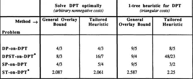
So for problems with proportional costs, by Theorem 1 the cost of the composite heuristic solution is at most 4/3 rds the optimal cost. For the TLND problem, PB = 1 and the minimum spanning tree (MST) heuristic (Takahashi and Matsuyama [1980]) solves the overlay (Steiner tree) subproblem with a worst-case ratio PO = 2. Therefore, Theorem 1 implies that the worst-case ratio of the composite heuristic for TLND problems with

10-proportional costs must not exceed 2. These worst-case bounds for the composite heuristic for HND and TLND problems are tight (Balakrishnan et al. [1992a]).

In Sections 4 and 5, we show that by exploiting special problem structure we can improve upon the worst-case bounds of Theorems 1 and 2 for several tier, two-connected network design models. For example, for one proportional cost model that we consider in Section 4.1, po =3/2 and PB = 1 and so Theorem 1 provides the bound coprop <

9/5 whereas the bound we obtain has an improved worst-case performance guarantee of 8/5. In another instance, we are able to reduce the bound from 4/3 to 5/4.

2.3 Heuristic analysis strategy

Theorems 1 and 2 and our worst-case analysis in Sections 4 and 5 use the following general approach. The analysis begins with the upper bound (2.5) on the cost of the composite heuristic. This bound depends on the costs of the BU and OC heuristic

solutions. For each specialized model that we consider, we attempt to improve the BU and OC heuristics and obtain sharper estimates of their costs. We also determine a lower bound on the optimal value Z* as follows. If we ignore the linking constraints (2.4) in

formulation [TTS], as we noted previously, the problem decomposes into the overlay subproblem with costs b and the base subproblem with costs a. Consequently, the sum of the optimal values for these two subproblems is a valid lower bound on Z*. We obtain another lower bound by ignoring the base constraints (2.3). Since all costs are

nonnegative, setting x = y is optimal for this relaxation, and so the optimal value of the relaxation is ZO(c). Combining these two lower bounds shows that

Z* > max {Z(b) + ZB(a),ZO(c)}. (2.8) Dividing the heuristic upper bound (2.5) by the lower bound (2.8) gives an upper bound on the heuristic worst-case performance ratio. For the proportional costs case, we express this ratio in terms of two parameters--the cost ratio r and the unknown ratio s =

ZO(a)/ZB(a) (we assume ZB(a) > 0). To obtain a data-independent performance characterization, we maximize the performance ratio with respect to s and r.

3. Solution Methods and Analysis for Underlying Single-tier Models

Sections 4 and 5 analyze two-tier versions of low connectivity network design models. These models have two new single-tier models-the dual path tree problem and the dual path Steiner tree problem--as their base and overlay subproblems. In this section, we study solution methods for these two single-level problems. This analysis will provide the

values of the worst-case parameters po and PB that we require for our subsequent two-level analysis.

Before beginning our analysis, let us introduce some terminology and briefly review relevant prior results. By triangularizing an undirected graph G = (N,E) with costs aij for all edges { ij

}

e E we mean constructing a complete graph G' = (N,E') with edge costs ai'j

for all i, j E N equal to the shortest path distance from node i to node j in G. We refer to G' as the triangularized graph and the costs ai'jas triangularized costs. When we consider

edge duplication, we will rely on the following property proved by Goemans and

Bertsimas [1993] for single-tier survivable network design (SND) problems: the optimal value of the SND problem defined over the triangularized graph G' (with edge duplication permitted in this graph as well) is the same as the optimal value over the original graph G. We will refer to this property as the duplication equivalence property. To construct a feasible SND solution over the original graph G from a feasible solution over G', we replace each edge {i,j

}

in the latter solution with the edges of the shortest i-to-j path in G (with replications if an edge in G appears in more than one such shortest path). We refer to the resulting solution to the original problem as the recovered solution.

Dual Path Steiner Tree (DPST) problem:

Given an undirected graph G=(N,E) with nonnegative edge costs aij, and a subset P S N of primary nodes containing two critical nodes 1 and 2, find the minimum cost subgraph that spans all the nodes of P via optional "Steiner" nodes from N\P, and that connects nodes 1 and 2 via two edge-disjoint paths.

In terms of the terminology we introduced for the general MTS model, the DPST problem has L = 1, and r = 1 for all node pairs i and j P except rl2= r 1= 2, and r = 0 if i or j

e P. The Dual Path Tree (DPT) problem is a special case of the DPST model with P = N, i.e., the solution must span all the nodes of graph G.

The DPST problem is NP-hard since it generalizes the Steiner network problem. As we will show later, if we assume triangular costs then the DPT problem is polynomially solvable. For DPT and DPST problems with arbitrary edge costs aij, Balakrishnan, Magnanti and Mirchandani [1994b] propose the following efficient dual path greedy

completion (DPGC) heuristic. Using a graph doubling argument, they show that the

DPGC method solves the DPST and DPT problems with a worst-case performance guarantee of 2. This bound holds for the problems with or without edge duplication.

12-Dual Path Greedy Completion (DPGC) heuristic:

Step 1: Find the minimum cost pair of edge-disjoint paths from node 1 to node 2. Let E1

and N1 be the subset of edges and nodes belonging to these paths.

Step 2: Contract the subgraph G1=(N1,E1) into a single node 0, triangularize the

resulting graph, and eliminate all the Steiner nodes not in N1 and their incident

edges, creating a graph G*. Find the minimum spanning tree of G*. Recover the original edges corresponding to the edges of this spanning tree and add one copy of each recovered edge to E1to obtain a feasible DPST solution.

The method derives its name from the operations of first finding the optimal "dual paths" (in Step 1) and then completing this solution in a greedy fashion (Step 2).

If we do not permit edge duplication, then as is well-known we can find the optimal dual paths in Step 1 by solving a minimum cost network flow problem defined on the following network. The network contains all the nodes and edges of G. Node 1 has a supply of 2 units, node 2 has a demand of 2 units, and all other nodes are transshipment nodes. The flow cost on each edge {i,j) is the original edge cost aij, and every edge has a capacity of 1 unit. The minimum cost flow solution routes 1 unit of flow on each of the two required edge-disjoint 1-to-2 paths. When we permit edge duplication, the optimal dual path solution consists of two copies of the shortest 1-to-2 path.

When the edge costs have special properties, can we develop alternative solution methods that have better worst-case performance than the DPGC method? For the DPT problem, we can indeed develop more effective methods. In particular, when the edge costs satisfy the triangle inequality, as we show in Section 3.1, the DPT problem is polynomially solvable using a matroid intersection algorithm. For a broader class of cost structures that we call g-direct costs, Section 3.2 describes and analyzes the worst-case performance of a simple 1-tree heuristic that is more effective than the DPGC method for a range of g values. The models considered in both Sections 3.1 and 3.2 prohibit edge duplication; Section 3.3 discusses algorithmic and worst-case implications for models that permit edge duplication.

3.1 Dual path trees for graphs with triangular costs

DPT problems with triangular costs are polynomially solvable. To establish this result, we use the following property.

Proposition 3:

If the edge costs satisfy the triangle inequality, then the DPT problem has an optimal solution containing exactly INI edges.

Proof:

The optimal solution to the DPT problem spans all the nodes in the graph and contains two edge-disjoint paths, say P1and P2, connecting the primary nodes 1 and 2. Because

the costs are nonnegative, we can choose both P1 and P2as simple paths (they do not

revisit nodes). If the paths P1 and P2intersect only at nodes 1 and 2, then the optimal

solution spans all nodes and contains exactly one cycle, and thus contains exactly INI edges.

Next suppose that the paths P1 and P2intersect at some intermediate node(s) other than

nodes 1 and 2. Let us orient these paths from node 1 to node 2; that is, node 1 is their first node and node 2 their last node. If paths P1and P2intersect at more than one intermediate

node, let a be the first intersection point (after node 1) on P1, and let b be the first

intersection point on P2. (Nodes a and b might be the same node). First, observe that

nodes b and a cannot simultaneously be (immediate) successors of each other on paths P1

and P2, since then both paths would contain the edge { a,b), contradicting the fact that P1

and P2are edge-disjoint. So, suppose that the node b is not the successor of node a on

path P1. Let i andj denote the predecessor and successor of node a on path P1. In path P1

replace the edges {i,a} and {aj} with the edge {i,j}; the triangle inequality implies that the cost of the resulting path P3does not exceed the cost of path P1.

Now note that if node a's predecessor is node i * 1, then since node a is the first intersection node on path PI, i O P2and so { i,j) P2. If i = 1, the definition of node b as

the first intersection node on path P2and the fact that b ; j implies that (ij) e P2. In either

case, the paths P2 and P3are edge disjoint. Moreover, by our previous observation these

two paths cost no more than the two paths P1 and P2. Therefore, we have found another

optimal solution to the DPT problem with one less node in common to the two paths. Repeatedly identifying nodes a and b allows us to short-circuit one of the two paths. Since each path contains a finite number of nodes, this constructive procedure terminates when the two paths intersect at only nodes 1 and 2.

14-Matroid Intersection algorithm:

We now show that the dual path tree is the intersection of two matroids. A 1-tree of a graph G is the union of a spanning tree and one edge not in the spanning tree. Clearly, a 1-tree contains exactly one cycle. A q-restricted 1-1-tree is a 1-1-tree with the property that the unique cycle formed by the additional edge contains a particular node q of the graph. We can interpret a dual path tree with exactly INI edges as the intersection of a 1-restricted

1-tree and a 2-restricted 1-tree. Subsets of q-restricted 1-trees form a matroid (see Exercise 13.39 in Ahuja, Magnanti, and Orlin [1993]). Since the weighted matroid intersection problem is solvable in polynomial time (Edmonds [1979]), Proposition 3 implies that we can optimally solve the DPT problem with triangular secondary costs in polynomial time. We have thus established the following result.

Theorem 4:

If the edge costs satisfy the triangle inequality, then a weighted matroid intersection algorithm solves the DPT problem optimally in polynomial time.

For DPST problems with triangular costs, suppose we use the corresponding optimal DPT solution over the primary nodes as a heuristic solution. Can we characterize the worst-case performance of this DPST heuristic method? Balakrishnan et al. [1994b] have shown that for any low connectivity Steiner problem with triangular costs, the heuristic solution obtained by optimally solving the corresponding low connectivity problem over the terminal nodes costs at most twice the original optimal value, and this bound is tight. This result implies that the matroid intersection-based heuristic for triangular cost DPST problems has a worst-case performance of 2, which is the same as the worst-case performance of the more general and simpler DPGC heuristic.

Although polynomial, the generic matroid intersection algorithm is complex and is typically difficult to implement (its specialization for the dual path tree problem might be much easier though). As an alternative, we might wish to use a simple heuristic method for solving the DPT problem even when the costs are triangular. In the Section 3.2, we

develop one such heuristic in the context of a broader class of graphs than those with triangular costs.

3.2 Dual path trees for g-direct graphs

Whenever the graph G contains the edge { 1,2 , this edge can potentially serve as one of the two edge-disjoint 1-to-2 paths. Therefore, if we do not permit edge duplication and

G has a feasible dual path tree, then if we start with edge { 1,2 }, the problem must have a feasible completion, i.e., the residual graph obtained by deleting edge { 1,2) must contain a 1-to-2 path. (When we permit edge duplication and G is connected, we can always

complete any given 1-to-2 path.) This observation motivates the following 1-tree heuristic. We state and analyze this O(IEI + INI logINI) heuristic in its general form, which is capable of solving both DPT and DPST problems.

1-Tree Heuristic:

Step 1: Remove the direct edge 1,2) from G and find an approximate or optimal solution STREE to the Steiner tree problem STP spanning all the primary nodes (with optional intermediate Steiner nodes) on the resulting residual graph G12.

Step 2: Add edge 1,2) to STREE to obtain the 1-tree heuristic solution to the DPST problem.

When applied to the DPT problem, Step 1 merely requires finding the minimum spanning tree of G12. In order to bound the worst-case performance of this heuristic, we

need to be able to bound (i) the cost of the Steiner tree it produces, and (ii) bound the cost of edge ({ 1,2) relative to the rest of the network. For (i), we let PST denote the worst-case ratio of the method we use to find the Steiner tree STREE. For (ii), we restrict our

attention to a special class of graphs that we call B-direct: these are graphs that: (a) have nonnegative edge costs, (b) contain edge { 1,2 , (c) contain a path connecting nodes 1 and 2 without edge { 1,2), and (d) satisfy the property that the cost a12of the edge (1,2) is no more than i (20) times the cost A₁₂of the shortest 1-to-2 path when we remove edge

{1,2). This assumption implies that any DPT and DPST solution that does not contain the edge ({ 1,2) costs at least 2A1 2> 2a12/g. Note that triangular graphs are t-direct graphs

with p = 1. In stating the following worst-case result for the 1-tree heuristic, we let ~ = max {,1 ).

Proposition 5:

Let s = min {(a2, A12)/ZDPST < 1/2 be the cost of the shortest path from node 1 to

node 2 relative to the optimal cost of the DPST problem. For p-direct graphs, the 1-tree heuristic generates a solution to the DPST problem with a worst-case bound of at most PST + min ({$/2, is). If any optimal DPST solution contains edge ({ 1,2, then the 1-tree solution has a worst-case bound of at most

-16-Proof:

We claim that the optimal value ZDPST of the DPST problem is no less than the optimal value ZSTP of the Steiner tree problem STP that we solve in Step 1 of the 1-tree heuristic.

Let Q* be an optimal DPST solution. Let Q' be any Steiner tree formed by dropping an edge from the cycle in Q* containing nodes 1 and 2, choosing edge ({ 1,2) if Q* contains this edge. Since Q' is a feasible solution to the Steiner tree problem STP, its cost Z(Q') is greater than or equal to ZSTP. Therefore, the cost Z(STREE) of the exact or approximate

Steiner tree STREE satisfies the following inequalities

ZDPST Z(Q') P ZSTREE> (3.1)

PST

If some optimal DPST solution OS contains edge 1,2), then this edge plus the Steiner tree solution on G12 obtained by removing this edge from OS solves the DSPT problem. Therefore, since PST 2 1 and a12 2 0,

ZDPST ZSTP + a12 Z(STREE) + a12 Z(STREE) + 12

PST PST PST

But, if Z1-treedenotes the cost of the 1-tree heuristic solution, then Zltre e- = Z(STREE) + a12 < PST ZDPST,

which is the last conclusion of the proposition.

If no optimal DPST solution contains edge 1,2), then since the graph is g-direct and the costs are nonnegative, ZDPST 2 2A122 2a1 2/1.. Combined with expression (3.1), this

inequality implies that the cost Z1-t ee of the 1-Steiner tree heuristic solution is bounded as follows:

Z1-t = Z(STREE) + a12 < PST ZDPST + ZDPST = (PST + 2) ZDPST- (3.2)

If edge { 1,2) isn't a shortest 1-to-2 path (i..e., g >1), then sZDPST = A12 > a12/g. In

this case, the previous inequality becomes Zl-bM _{= Z(STREE) + a}

12 < PST ZDPST + gs ZDPST = (PST + ps) ZDPST. (3.3)

If edge ({ 1,2) is the shortest 1-to-2 path (i.e. g < 1), then

Zt ree _{= Z(STREE) + a}

12 < PST ZDPST + S ZDPST = (PST + S) ZDPST- (3.4)

The inequalities (3.2), (3.3), and (3.4) imply that

When we apply the 1-tree heuristic to the DPT problem, PST = 1 and so we obtain the following corollary.

Corollary 6:

For DPT problems defined on g-direct graphs, the 1-tree heuristic generates a solution with a worst-case bound of at most 1 + min { 1/2, 's)} < 1 + /2.

The following example shows that the bound in Corollary 6 is tight. Consider a g-direct network containing 3 paths from node 1 to node 2: a g-direct path costing g, and two alternate unit-cost paths, each containing q "short" edges (every edge on these two paths has a cost of l/q). If 1/q < g, then the optimal solution is the two non-direct paths at a cost of 2; the 1-tree heuristic solution uses all but one of the short edges and costs 2 + pg - l/q. Therefore, the ratio of the 1-tree solution's cost to the optimal value is 1 + p/ 2 - 1/2q, which approaches 1+p/2 as q approaches infinity.

Note that for solving DPST problems, the 1-tree heuristic is not competitive (in terms of worst-case performance) with the DPGC method unless we solve the Steiner problem optimally, or we know that the optimal DPST solution contains edge { 1,2), or we use Berman and Ramaiyer's [1992] heuristic (with PST = 16/9) to solve the Steiner tree problem and t < 4/9. Also, if g > 2, then the DPGC method is superior even for DPT problems defined on pg-direct graphs. In subsequent sections we assume, for convenience,

that we always apply the DPGC method to approximately solve the DPST problem.

3.3 Dual path trees with edge duplication

When we permit edge duplication, we can solve the DPT problem with arbitrary costs in polynomial time using a modified matroid intersection algorithm. The following

proposition proves a special property of an optimal DPST solution with edge duplication in triangularized graphs, enabling us to extend the matroid intersection algorithm to the edge duplication case as well.

Proposition 7:

The DPST problem with edge duplication has an optimal solution that either chooses edge { 1,2) twice or contains only unduplicated edges.

-18-Proof:

By the duplication equivalence property, assume the costs are triangular. Consider an optimal solution that duplicates some edge i,j } * { 1,2). If edge i,j } does not belong to both the 1-to-2 paths in the dual path tree, we can delete one copy of this edge from the solution. Otherwise, we can short-circuit either node i or j * 1, 2 on one of the paths, obtaining a feasible solution with equal or lower costs and using fewer edges in the 1-to-2 paths. Repeating this procedure for all duplicated edges {i,j } { 1,2 provides the required optimal DPST solution.

For the DPT problem with edge duplication, consider a solution satisfying the

conditions of Proposition 7. If this solution contains edge { 1,2) twice, then the remaining edges must be spanning tree edges, and so the solution contains exactly n edges.

Otherwise, the solution must be optimal for the "unduplicated" version of the problem, i.e., for the triangularized DPT problem without edge duplication. Proposition 3 shows that this unduplicated problem has an optimal solution containing exactly n edges. So we have the following corollary to Proposition 7.

Corollary

8:

The DPT problem with edge duplication has an optimal solution containing exactly n edges.

We can exploit this property to optimally solve the DPT problem with general (nonnegative) costs and with edge duplication as follows:

Edge-duplicating Matroid Intersection algorithm:

Triangularize the given graph G and add one parallel copy of edge { 1,2 to form a new augmented graph G". Apply the matroid intersection algorithm (without edge

duplication) to this augmented graph. Recover the solution to the original graph G. As we noted before, solving the DPT problem optimally over the primary nodes provides a heuristic DPST solution that costs at most twice the optimal DPST value.

Consequently, for DPST problems with arbitrary costs but edge duplication, we can apply the Edge-duplicating Matroid Intersection algorithm to the corresponding DPT problem to

Notice that we could replace the use of the matroid intersection algorithm for solving the triangularized version of the problem in the augmented graph G" by any heuristic method that applies to triangular cost DPT problems with edge duplication. In particular, we could apply the 1-tree heuristic with the following adaptation: in Step 1 of the method, we delete only one copy of edge

{

1,2) before finding the optimal or approximate Steiner tree. Equivalently, in Step 1 we find the optimal or approximate Steiner tree for the

triangularized graph G', and then add edge { 1,2) (a parallel copy if this edge already exists in the Steiner tree) in Step 2. It is easy to adapt our prior analysis to show that this

Edge-duplicating I-tree heuristic has the same worst-case bounds as the original version of the

1-tree heuristic (see Proposition 5 and Corollary 6). In particular, for DPT problems with edge duplication, the edge-duplicating 1-tree heuristic produces a solution that costs at most

1.5 times the optimal value.

Goemans and Bertsimas [1993] proposed a "tree heuristic" to solve a large class of single-level, survivable network design problems with edge duplication. When specialized to the DPT or DPST problems, this heuristic is the same as the Edge-duplicating -tree heuristic (assuming that to solve the DPST problem this heuristic applies the MST heuristic to solve the Steiner subproblem in Step 1). Goemans and Bertsimas showed that the tree heuristic generates a solution that costs no more than twice the optimal value of the

survivable network design problem. Relative to this bound, Corollary 6 provides a tighter bound of 3/2 for DPT problems, but for DPST problems Proposition 5 implies a weaker bound of 5/2. Our DPGC heuristic achieves the bound of 2 for both DPT and DPST problems with general costs, with or without edge duplication.

This section has examined the DPT and DPST single-tier subproblems of the two-tier models that we study next. The general purpose DPGC algorithm finds a heuristic DPST or DPT solution within a factor of 2 of the optimal value. For DPT problems defined over triangular and g-direct graphs, the matroid intersection method and the -tree heuristic solve the problem optimally or within a factor of 1+p,/2. As we have shown, for situations that permit edge duplication, we can optimally solve DPT problems with arbitrary costs using matroid intersection.

4. Heuristic Analysis of Cycle+Tree Problems with Full Back-up

This section and Section 5 examine full and partial back-up versions of two-connected generalizations of the hierarchical network design and two-level network design problems.

20-In these two-tier models, the undirected graph G=(N,E) has a subset P of primary or high-level nodes that must be interconnected via primary paths (with optional intermediate secondary nodes). Furthermore, two critical nodes in P, nodes 1 and 2, require mutual two-connectivity, and the design must span all the remaining secondary nodes using secondary facilities. We refer to this class of models as Cycle+Tree models since the required network configuration consists of a tree plus edges of a cycle.

In the full back-up versions of these two-tier survivable network design problems, the two edge-disjoint paths connecting the critical nodes must both contain only primary facilities. Thus, the connectivity requirements of this model are: (i) at the primary service

level: r = 1 if i and j e P except rl12 = r21= 2; and (ii) at the secondary service level: r22

= r21 = 2 and r2 = 1 otherwise. For the general version of this problem, the overlay subproblem is the dual path Steiner tree (DPST) model and the base subproblem is a dual dath tree (DPT) problem; we therefore refer to this model as the DPST-on-DPT model. We also consider the DP-on-DPT special case containing only two primary nodes, both of which are critical. This model has the polynomially solvable dual path (DP) problem as its overlay subproblem.

Using Section 3's algorithms and worst-case results for DPT and DPST problems, we develop specialized worst-case bounds for the composite heuristic for the DPST-on-DPT and DP-on-DPT problems; these results improve upon the bounds we would obtain by applying general overlay results in Section 2.

4.1 The DPST-on-DPT problem

For the DPST-on-DPT problem, the BU heuristic that we described in Section 2 solves the DPT problem using primary edge costs, and installs primary facilities on all the edges of this solution. From our discussions in Section 3, we note that the worst-case ratio PB of the embedded procedure to solve the base (DPT) subproblem depends on the problem's cost structure (triangular, WI-direct, or general) and on the method that we apply (matroid intersection, 1-tree heuristic, or DPGC heuristic).

The OC heuristic solves the DPST problem using primary costs, and completes this solution by adding edges (containing secondary facilities) in order of increasing secondary costs to connect the remaining secondary nodes. As for the base subproblem, the worst-case ratio po of the embedded procedure to solve the overlay subproblem depends on the cost structure and the method that we apply. The total secondary cost of all the edges that

the OC heuristic adds to complete any overlay (DPST) solution does not exceed the cost of the minimum spanning tree of G using secondary costs, which does not exceed the optimal value ZB(a) of the base (DPT) subproblem. Therefore, the DPST-on-DPT problem

satisfies the feasible completion property with a completion cost multiplier X = 1. Since the OC heuristic's greedy completion step (adding edges in increasing order of secondary cost to span the nodes not in the DPST solution) incurs a completion cost of at most ZB(a), the OC heuristic solution costs at most ZO(c)+ZB(a). In contrast, the analysis of general overlay optimization problems in Section 2 assumes that we solve the completion subproblem using the same heuristic that we use to solve the base subproblem. So, the general completion procedure can add a completion cost of up to pBZB(a), giving the looser OC upper bound ZO()+PBZB(a) (see inequality (2.5)). Since the BU heuristic costs at most PBZB(c), the composite solution to the DPST-on-DPT problem costs no more than min

{

PBZB(c), ZO(c)+ZB(a)) }. This observation and the lower bound (2.8) imply the following bound on the composite heuristic's worst-case ratio for DPST-on-DPT problems:

zComp min PBZB(C), POZ(c)+ZB(a) } * - max ({Z(c), ZO(b)+ZB(a)}

For the proportional costs case, if s denotes the optimal secondary cost of the overlay subproblem relative to the optimal base subproblem value ZB(a), then inequality (4.1) reduces to

min {PBr, pOrs+ 1 }(4.2)

{(r-1)s+l (4

We must select values of s and r that maximize the right-hand side of inequality (4.2) subject to the constraints that O < s < 1 and r > 1. If we ignore the restrictions on s, the right-hand side of (4.2) achieves its maximum when

s* = Br- 1 (4.3)

por

Notice that since PB and r are both greater than or equal to 1, s* is nonnegative.

Furthermore, for both triangular and arbitrary costs, if we use our single-level heuristics from Section 3 or if we optimally solve the overlay and base subproblems, then 1< PB <

pO. Therefore, the value of s* given by equation (4.3) is always less than or equal to 1 whenever the value of r is at least 1.

-Substituting this value of s* in (4.2), we obtain PB P r2

(Oprop (1 - r[pB+l-po] + PBr2) (44)

Let us now consider two cases: Case 1:0 < PB+ 1_{-PO < 2.}

Differentiating the right-hand side of (4.4) with respect to r, we find that this expression achieves its maximum when

r* 2 (4.5)

(PB+ 1-PO)

Since 0 < PB+l-PO < 2, this value of r* satisfies the requirement r > 1. Substituting for r* in (4.4), we obtain

4 PBPO

Oprop <- (4.6a)

PB (2+2PO-PB) - (po-1)2 ₍

Case 2: PB+1-PO < ₀

In this case, the right-hand side of inequality (4.4) increases with r, and achieves its maximum value when r* = oo. Therefore,

Cprop < PO. (4.6b)

We do not consider the third case when PB+1-PO > 2 because, as we discuss next, this case does not apply when we use our single-level heuristics to solve the overlay and base subproblems.

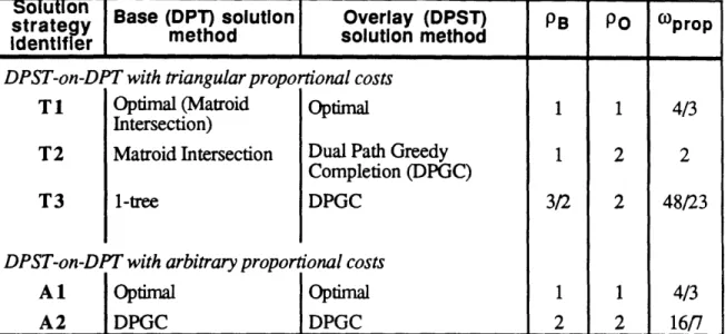
Let us now consider various possible combinations of overlay and base solution methods. We can either solve the DPT base subproblem optimally (using the matroid intersection algorithm if costs are triangular) or apply the 1-tree or DPGC heuristics for problems with triangular or arbitrary costs. For the DPST overlay subproblem, we consider the options of solving it optimally (using, say, branch-and-bound) or approximately using the DPGC heuristic. Table I lists the resulting combinations of overlay and base solution methods, the corresponding base and overlay heuristic worst-case ratios, and the composite heuristic's performance ratio for proportional cost problems. To keep the discussions simple, we do not consider DPST-on-DPT problems defined on general B-direct graphs, but instead limit our attention to the special case of triangular costs.

Table I: Proportional costs DPST-on-DPT solution options

For solution strategies T1 and Al, (PB+ 1-PO) = 1, and so the bound (4.6a) applies. Since PB = PO = 1 for both these strategies, the composite heuristic has a worst-case ratio of 4/3, which is the same bound as in Theorem 1. For strategy T2 as well, Theorem 1 gives the same worst-case bound of 2 as (4.6b). However, for strategies T3 and A2, Theorem l's bounds are 9/4 and 8/3 while inequality (4.6b) gives better bounds of 48/23

and 16/7. Note that the bounds in Theorem 1 apply to problems without edge duplication. If we permit edge duplication, then the DPT subproblem can be solved optifnally even when costs do not satisfy the triangle inequality. Therefore, we might be interested in solving such problems using strategy T2 or T3 instead of strategy A2.

Consider the unrelated costs case. Using the OC heuristic, we obtain,

unrel mapOZo(a)+ZB(a)

unrel < max {Z(c), Zo(b)+ZB(a)I

< PO+ 1. (4.7)

Notice that, unlike Theorem 2, the worst-case ratio for the unrelated costs case does not depend on the performance of the base heuristic.

Theorem 9:

For the DPST-on-DPT problem, the worst-case performance ratios coprop and ounrel corresponding to problems with proportional and unrelated costs are bounded from above as follows:

-24

-strateolution

Base (DPT) solution Overlay (DPST) PB PO oprop identifier

DPST-on-DPT with triangular proportional costs

T 1 Optimal (Matroid Optimal 1 1 4/3

Intersection)

T2 Matroid Intersection Dual Path Greedy 1 2 2

Completion (DPGC)

T3 1-tree DPGC 3/2 2 48/23

DPST-on-DPT with arbitrary proportional costs

Al1 Optimal Optimal 1 1 4/3

4 P PO

prop -1)2 if 0 < PB+ 1-PO < 2, (4.8a) PB (2+2Po-PB) - (Po- 1 )2

< Po if PB+1-PO < 0; and, (4.8b)

(ounrel < P + 1. (4.8c)

4.2 The DP-on-DPT problem

For the DP-on-DPT special case with only two primary (and critical) nodes, the overlay subproblem seeks the minimum cost pair of edge-disjoint paths connecting nodes 1 and 2. As we noted in Section 3, this dual path problem is a minimum cost network flow problem, and so PO = 1. The completion cost multiplier X is 1 since the overlay completion

procedure of adding edges (to the dual path) in increasing secondary cost order to span the remaining secondary nodes incurs a cost no more than the optimal value of the base

subproblem. The BU heuristic is the same for both the DP-on-DPT and DPST-on-DPT problems: we find an approximate or optimal DPT solution and install primary facilities on all the edges of this design. Therefore, the results of Theorem 9 apply. Substituting PO =

1 in expressions (4.8a) and (4.8c) gives

Corollary 10:

For the DP-on-DPT model, the worst-case performance ratios O)prop and Ounrel for problems with proportional costs and unrelated costs are bounded from above as follows:

4

00prop - - , and (4.9a)

4 _-PB

ounrel < 2. (4.9b)

For proportional cost problems, when we solve the DPT subproblem optimally (e.g., if costs are triangular or edge duplication is permitted, and we apply the matroid intersection algorithm), Corollary 10 gives the same worst-case bound of 4/3 as Theorem 1. However, when we use the dual path greedy completion (DPGC) heuristic with PB = 2 to

approximately solve the DPT base subproblem, Corollary 10 reduces the bound on prop from 16/7 (in Theorem 1) to 2. Similarly, when we apply the 1-tree heuristic (with PB =

3/2) to approximately solve the triangular cost DPT base problem, Corollary 10 gives a proportional costs worst-case ratio of 8/5 while Theorem 1 implies a ratio of 9/5.

4.2.1 DP-on-DPT worst-case examples

Since we will present DP-on-DPT worst-case examples for several cases, we first provide a brief overview of these examples. Figures 2 and 3 describe worst-case examples for the proportional cost DP-on-DPT problem. These examples achieve the bounds of 4/3 and 2 corresponding to situations when we either (i) solve the DPT subproblem optimally, or (ii) use the DPGC heuristic with a worst-case performance ratio of 2 to solve the DPT subproblem. For triangular, proportional cost problems, we have not been able to construct an example that achieves the bound of 8/5 when we use 1-tree heuristic as the embedded base subproblem solution method. Figure 4 describes an example with a heuristic performance ratio of 3/2.

Figures 5 and 6 describe worst-case examples for the unrelated costs DP-on-DPT problem. Although we considered only the OC heuristic in order to develop the worst-case bound of 2 (Theorem 9) for problems with unrelated costs, our examples demonstrate that the bound is tight even when we apply the BU heuristic and choose the better of the BU and OC heuristic solutions. Figure 5 assumes that we solve the DPT subproblem optimally, while Figure 6 assumes that we apply the DPGC heuristic to approximately solve the DPT subproblem.

Let us now discuss these examples in more detail. Figure 2 contains a worst-case example for the proportional cost DP-on-DPT problem to show that, when we solve the DPT subproblem optimally, the bound of 4/3 is tight. Figure 2(a) shows the network configuration and the secondary costs; the primary-to-secondary cost ratio r is 2 for all edges. Edges { l,a} and {2,b} each have secondary costs of l/q: q is a sufficiently large multiple of 4. Edges

{

a,2 and {b,1 } each have a cost of 1/4. The network contains two parallel paths, each containing q/4 nodes, connecting nodes a and 2; every edge on these paths has a secondary cost of 1/q. Each intermediate node on these two parallel paths is connected to the node vertically adjacent to it with an edge of cost l/q. A similar

configuration of parallel paths connects node b to node 1. The OC heuristic solution, shown in Figure 2(b), costs 2{1/2 + 2(1/q)} + (4q/4)(l/q) -= 2 + 4/q. The BU heuristic

solution (Figure 2(c)) costs 2{2(q/4 + 1)(l/q) + 2(q/4)(1/q) + 2(1/q)) = 2 + 8/q. Finally, the optimal solution (Figure 2(d)) costs 2{(q/4 + 1)(1/q) + 2(1/q)) + 2(q/4)(1/q) =

3/2 + 8/q. Therefore, the heuristic performance ratio for this example approaches 4/3 as q approaches infinity.

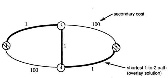
-Figure 3 describes a proportional cost worst-case example that achieves the bound of 2 when we solve the DPT subproblem using the DPGC heuristic. Figure 3(a) shows the network configuration and secondary costs; in this example, the cost ratio r is 1. The network has four alternate paths connecting the primary nodes 1 and 2: (i) a direct path of secondary cost 1, (ii) a two-edge path with edge costs 1/q and (l-1/q), and (iii) two q-edge paths with total secondary cost 1. The OC heuristic, shown in Figure 3(b), costs 4-2/q. The BU heuristic, shown in Figure 3(c), also costs 4-2/q. Figure 3(d) shows the optimal solution, which costs 2 + 1/q. Thus, the performance ratio of the composite heuristic approaches 2 as q approaches infinity.

Figure 4 presents a DP-on-DPT example with triangular, proportional costs. The given graph G is the triangularized version of the graph shown in the figure. Unlike the previous example, the cost ratio r is 2 instead of 1. The OC heuristic solution shown in Figure 4(b) costs 6-2/q, the BU heuristic solution (using the embedded 1-tree heuristic) shown in Figure 4(c) costs 6, while the optimal solution (Figure 4(d)) costs 4+1/q. As q approaches infinity, the performance ratio for this example approaches 3/2.

Figures 5 and 6 contain examples for the unrelated costs DP-on-DPTproblem. Assuming that we can solve the DPT subproblem optimally, our worst-case example has the same network configuration as Figure 2(a), but uses the cost parameters shown in Figure 5. Figures 2(b), 2(c), and 2(d) depict the structure of the OC heuristic solution, BU heuristic solution (assuming that we solve the DPT subproblem optimally), and optimal solution for this example. For large values of q, the performance ratio approaches the worst-case performance bound of 2.

We can similarly modify the costs of Figure 3(a) to show that our worst-case bound is tight even when we use the DPGC heuristic to solve the DPT subproblem. Figure 6 shows the cost parameters for this example. Figures 3(b), 3(c), and 3(d) depict the structure of the OC heuristic solution, BU heuristic solution, and optimal solution for this example. For large values of q, the performance ratio approaches the worst-case bound of 2.

In closing, we note that whenever we use the DPGC heuristic to solve the DPT base subproblem of the DP-on-DPT model, then the composite heuristic achieves the tight performance ratio bound of 2 for both proportional and unrelated costs. Thus, this model provides one example for which the worst-case performance ratio for the base subproblem equals the worst-case bound for the two-tier, two-connected overlay optimization problem.

5. Heuristic Analysis of Cycle+Tree Problems with Partial Back-up

The partial back-up Cycle+Tree model permits secondary facilities on one of the two edge-disjoint paths connecting the two critical nodes 1 and 2. This section studies the partial back-up counterparts--the SP-on-DPT and ST-on-DPT problems-of the

full-back-up DP-on-DPT and DPST-on-DPT problems that we considered in Section 4. In the SP-on-DPT model, the graph contains two primary nodes, both of which are critical. We must find the minimum cost spanning subgraph that contains a primary path connecting nodes 1 and 2, and an alternate edge-disjoint 1-to-2 path containing either primary or secondary facilities. Its overlay subproblem is the shortest path (SP) problem, and its base

subproblem is the dual path tree (DPT) problem. The more general ST-on-DPT problem contains more than two primary nodes. The design must contain (i) a primary subgraph spanning all the primary nodes, (ii) an alternate 1-to-2 path containing primary or facilities, and (iii) spanning tree edges connecting all the remaining secondary nodes. The

connectivity requirements for the ST-on-DPT model are: (i) at the primary service level: rj = 1 if i and j E P; and (ii) at the secondary serrvice level: r 2 = r221 = 2 and ri = 1 otherwise.

For this two-tier, partial back-up model, the overlay subproblem is the Steiner tree (ST) problem.

Although the distinction between full and partial back-up models appear to be relatively minor, the analysis for the partial back-up versions is quite different because, in general, the overlay subproblem might generate a solution that cannot be feasibly completed. However, as we show in Section 5.1, problems defined on g-direct graphs satisfy the feasible completion property. In this case, we obtain improvements on the general overlay results of Section 2 by modifying and obtaining sharper worst-case bounds on both the BU and OC heuristic procedures. Also, unlike Section 4 where we directly applied the worst-case results for the DPST-on-DPT problemto the DP-on-DPT problem, in this section we exploit the special features of the SP-on-DPT problem to obtain better bounds than the general on-DPT model. We study the SP-on-DPT problem in Section 5.1, and the

ST-on-DPT model in Section 5.2.

5.1 The SP-on-DPT problem

Let us first address the potential difficulties in overlay completion for SP-on-DPT problems with general costs. The SP-on-DPT problem's overlay subproblem is a shortest path problem (from node 1 to 2). The OC heuristic first finds the shortest 1-to-2 path using