HAL Id: hal-02066649
https://hal.inria.fr/hal-02066649v5
Preprint submitted on 2 Mar 2021
HAL is a multi-disciplinary open access
archive for the deposit and dissemination of
sci-entific research documents, whether they are
pub-lished or not. The documents may come from
teaching and research institutions in France or
abroad, or from public or private research centers.
L’archive ouverte pluridisciplinaire HAL, est
destinée au dépôt et à la diffusion de documents
scientifiques de niveau recherche, publiés ou non,
émanant des établissements d’enseignement et de
recherche français ou étrangers, des laboratoires
publics ou privés.
On the Optimization of Iterative Programming with
Distributed Data Collections
Sarah Chlyah, Nils Gesbert, Pierre Genevès, Nabil Layaïda
To cite this version:
Sarah Chlyah, Nils Gesbert, Pierre Genevès, Nabil Layaïda. On the Optimization of Iterative
Pro-gramming with Distributed Data Collections. 2021. �hal-02066649v5�
On
the Optimization of Iterative Programming with
Distributed
Data Collections
SARAH CHLYAH, Univ. Grenoble Alpes, CNRS, Inria, Grenoble INP, LIG, 38000 Grenoble, France NILS GESBERT, Univ. Grenoble Alpes, CNRS, Inria, Grenoble INP, LIG, 38000 Grenoble, France PIERRE GENEVÈS, Univ. Grenoble Alpes, CNRS, Inria, Grenoble INP, LIG, 38000 Grenoble, France NABIL LAYAÏDA, Univ. Grenoble Alpes, CNRS, Inria, Grenoble INP, LIG, 38000 Grenoble, France Big data programming frameworks are becoming increasingly important for the development of applications for which performance and scalability are critical. In those complex frameworks, optimizing code by hand is hard and time-consuming, making automated optimization particularly necessary. In order to automate optimization, a prerequisite is to find suitable abstractions to represent programs; for instance, algebras based on monads or monoids to represent distributed data collections. Currently, however, such algebras do not represent recursive programs in a way which allows for analyzing or rewriting them. In this paper, we extend a monoid algebra with a fixpoint operator for representing recursion as a first class citizen and show how it enables new optimizations. Experiments with the Spark platform illustrate performance gains brought by these systematic optimizations.
1 INTRODUCTION
Ideas from functional programming play a major role in the construction of big data analytics applications. For instance they directly inspired Google’s Map/Reduce [7]. Big data frameworks (such as Spark [25] and Flink [5]) further built on these ideas and became prevalent platforms for the development of large-scale data intensive applications. The core idea of these frameworks is to provide intuitive functional programming primitives for processing immutable distributed collections of data.
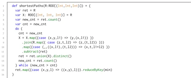
Writing efficient applications with these frameworks is nevertheless not trivial. Let us consider for instance the problem of finding the shortest paths in a large scale graph. We could write the Spark/Scala program in Fig 1 to solve it. The shortestPaths() function takes as input a graph R of weighted edges (src, dst, weight) and returns the shortest paths between each pair of nodes in the graph. The loop (in lines 6 to 14 of Fig 1) computes all the paths in the graph and their lengths; to get new paths, edges from the graph get appended to the paths found in the previous iteration using the join operation. Then reduceByKey operation is used to keep the shortest paths.
1 defshortestPaths(R:RDD[(Int,Int,Int)]) = {
2 var ret = R
3 var X: RDD[(Int, Int, Int)] = R
4 var new_cnt = ret.count()
5 var cnt = new_cnt
6 do {
7 cnt = new_cnt
8 X = X.map({case (x,y,l1) => (y,(x,l1)) })
9 .join(R.map({case (z,t,l2) => (z,(t,l2)) }))
10 .map({case (_,((x,l1),(t,l2))) => (x,t,l1+l2) })
11 .subtract(ret)
12 ret = ret.union(X).distinct()
13 new_cnt = ret.count()
14 } while (new_cnt > cnt)
15 ret.map({case (x,y,l) => ((x,y),l)}).reduceByKey(min)
16 }
Fig. 1. Shortest paths program.
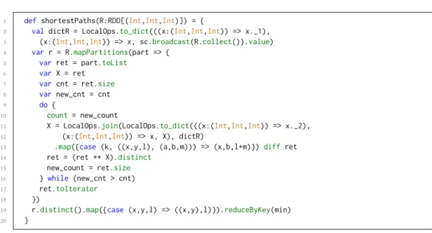
Spark performs the join and distinct operations by transferring the datasets (arguments of the operations) across the workers so as to ensure that records having the same key are in the same partition for join, and that no record is repeated across the cluster for distinct. Hence, for optimizing such programs, the programmer needs to take this data exchange into account as well as other factors like the amount of data processed by each worker and its memory capacity, the network overhead incurred by shuffles, etc. One optimization that can be done to reduce data exchange in this program is to assign each worker a part of the graph and make it compute the paths in the graph that start from its own part. This optimization leads to the following program (Fig 2.) which is not straightforward to write, less readable, and requires the programmer to give his own local version of dataset operators (such as join) that are going to be used to perform the local computations on each worker.
Another possible optimization is to put the reduceByKey operation inside the loop to keep only the shortest paths at each iteration because each subpath of a shortest path is necessarily a shortest path. More generally, finding such program rewritings can be hard. First, it requires guessing which program parts affect performance the most and could potentially be rewritten more efficiently. Second, assessing that the rewriting performs better can hardly be determined without experiments. During such experiments, the programmer might rewrite the program possibly several times, because he has limited clues of which combination of rewritings actually improves performance.
In this paper, we explore the foundations for the automatic transformation and optimization of Spark programs. Algebraic foundations in particular are an active research topic [2, 8]. The purpose of the algebraic formalism is to represent a program in terms of algebraic operators that can be analysed and transformed so as to produce a program that executes faster. Transformation-based optimizations are done through rewrite rules that transform an algebraic expression to an equivalent, yet more efficient, one. In the context of big data applications, considered algebras must be able to capture distributed programs on big data platforms and provide the appropriate primitives to allow for their optimization. One example of optimizations is to push computations as close as possible to where data reside.
When programming with big data frameworks, data is usually split into partitions and both data partitions and computations are distributed to several machines. These partitions are processed in
1 defshortestPaths(R:RDD[(Int,Int,Int)]) = {
2 val dictR = LocalOps.to_dict(((x:(Int,Int,Int)) => x._1),
3 (x:(Int,Int,Int)) => x, sc.broadcast(R.collect()).value)
4 var r = R.mapPartitions(part => {
5 var ret = part.toList
6 var X = ret
7 var cnt = ret.size
8 var new_cnt = cnt
9 do {
10 count = new_count
11 X = LocalOps.join(LocalOps.to_dict(((x:(Int,Int,Int)) => x._2),
12 (x:(Int,Int,Int)) => x, X), dictR)
13 .map({case (k, ((x,y,l), (a,b,m))) => (x,b,l+m)}) diff ret
14 ret = (ret ++ X).distinct
15 new_count = ret.size
16 } while (new_cnt > cnt)
17 ret.toIterator
18 })
19 r.distinct().map({case (x,y,l) => ((x,y),l)}).reduceByKey(min)
20 }
Fig. 2. Shortest paths program with less data exchange.
parallel and intermediate results coming from different machines are combined, so that a unique final result is obtained, regardless of how data was split initially. This imposes a few constraints on computations that combine intermediate results. Typically, functions used as aggregators must be associative. For this reason, we consider that the monoid algebra is a suitable algebraic foundation for taking this constraint into account at its core. It provides operations that are monoid homomorphisms, which means that they can be broken down to the application of an associative operator. This associativity implies that parts of the computation can actually be performed in parallel and combined to get the final result.
A significant class of big data programs are iterative or recursive in nature (PageRank, k-means, shortest-path, reachability, etc.). Iterations and recursions can be implemented with loops. Depend-ing on the nature of the computations performed inside a loop, the loop might be evaluated in a distributed manner or not. Furthermore, certain loops that can be distributed might be evaluated in several ways (global loop on the driver1, parallel loops on the workers, or a nested combination of the latter). The way loops are evaluated in a distributed setting often has a great impact on the overall program execution cost. Obviously, the task of identifying which loops of an entire program can be reorganized into more efficient distributed variants is challenging. This often constitutes a major obstacle for automatic program optimization. In the algebraic formalism, having a recursion operator makes it possible to express recursion while abstracting away from how it is executed. The execution plan is then decided after analysing the program.
The goal of this work is to introduce a gain in automation of distributed program transformation towards more efficient variants. We focus especially on recursive programs (that compute a fixpoint). For this purpose, we propose an algebra capable of capturing the basic operations of distributed computations that occur in big data frameworks, and that makes it possible to express rewriting rules that rearrange the basic operations so as to optimize the program. We build on the monoid
1In Big Data frameworks such as Spark, the driver is the process that creates tasks and sends them to be executed in parallel
algebra introduced in [8, 10] that we extended with an operator for expressing recursion. This monoid algebra is able to model a subset of a programming language L (for instance Scala), that expresses computations on distributed platforms (for instance Spark).
Contributions. Our contributions are the following:
(1) An extension of the monoid algebra with a fixpoint operator. This enables the expression of recursion in a more functional way than an imperative loop and makes it possible to define new rewriting rules;
(2) New optimization rules for terms using this fixpoint operator:
• We show that under reasonable conditions, this fixpoint can be considered as a monoid homomorphism, and can thus be evaluated by parallel loops with one final merge rather than by a global loop requiring network overhead after each iteration;
• We also present new rewriting rules with criteria to push filters through a recursive term, for filtering inside a fixpoint before a join, and for pushing aggregations into recursive terms;
• Finally, we present experimental evidence that these new rules generate significantly more efficient programs.
2 THEµ-MONOIDS ALGEBRA
In this section, we describe a core calculus, which we call µ-monoids, intended to model a subset of a programming language L (e.g. Scala2) that is used for computations on a big data framework
(through an API provided by the framework). µ-monoids aims at being as general as possible, while focusing on formalizing computations subject to optimization. Dataset manipulations are captured as algebraic operations, and specific operations on elements of those datasets are captured as functional expressions that are passed as arguments to some of the algebraic operations. In µ-monoids, we formalize some of those functional constructs, specifically the ones that we need to analyse in the algebraic expressions. For example, some optimization rules need to analyse the pattern and body of flatmap expressions in order to check whether the optimization can take place. Making explicit only the shapes that are interesting for the analysis enables to abstract from the specific programming language L that we optimize. This way, constructs of L other than those which we model explicitly are represented as constants c, as they are going to be left to L’s compiler to typecheck and evaluate. We only assume that every constant c has a type type(c) which is either a basic type or a function type, and that, when its type is t1→t2, it can be applied to any argument
of type t1to yield results of type t2.
We first describe the data model we consider, then in Sec. 2.2 we introduce the syntax of our core calculus. We then proceed to give a denotational semantics for our specific constructs in Sec. 2.3 and discuss evaluation of expressions in Sec. 2.5.
2.1 Data model: distributed collections of data
In big data frameworks, a data collection is divided into sub-collections stored into each machine. A collection can be in the form of a bag (a structure where the order is not important and where elements can be repeated), a list (a sequenced bag), or a set (a bag where elements do not repeat). In the context of this paper and for the sake of simplicity, we will focus on bags, although the operations we present can easily be defined for lists. Sets with no duplicates are impractical to
2Major Bigdata frameworks like Spark and Flink provide a Scala API and is implemented in Scala which makes Scala a
suitable language for our work. Scala also provides reflection which allows generic Scala constructs to be part of the algebra as we will explain later.
implement in a distributed context but we can assume that the language L provides a distinct operation which removes all duplicates from a bag.
In order to enable algebraic datatypes, we assume an infinite set of constructors C which can be applied to any number of values. We assume this set contains the special constructorsTrue,False
andTuplefor which we will define some syntactic sugar.
The syntax of considered data values is defined as follows:
v ::= c constant
| C(v1,v2, ...,vn) n-ary constructor | {v1} ⊎ {v2} ⊎... ⊎ {vn} bag
in which a bag is seen as the union of its singletons where ⊎ denotes the bag union operator. As mentioned previously (Sec. 2), a constant c can be any value from the language L (in particular any function) that is not explicitly defined in our syntax.
We define the following syntax for types:
tl ::= local type t ::= type
B basic type | tl
| C1[tl, ..., tl] || ··· || Cn[tl, ..., tl] sum type | Bagd[tl] distributed bag type
| Bagl[tl] local bag type | t → t function type
where B represents any arbitrary basic type (i.e., considered as a constant atomic type in our formalism).
We also define product types t1× ··· ×tnas syntactic sugar forTuple[t1, ..., tn].
In sum types, all constructors have to be different and their order is irrelevant.
For a given type t , we denote byBagl[t ] the type of a local bag and byBagd[t ] the type of a distributed bag of values of type t . Notice that we can have distributed bags of any data type t including local bags, which allows us to have nested collections. We allow data distribution only at the top level though (distributed bags cannot be nested).
Some operators over bags can be defined similarly, regardless of whether bags are local or distributed. For convenience, we thus denote the type of bags, either distributed or not as:Bag[t ] ::= Bagl[t ] |Bagd[t ]. For example, the bag union operator ⊎ :Bag[t ] ×Bag[t ] →Bag[t ] is defined for
both local and distributed bags. We consider that whenever any argument of ⊎ is a distributed bag then the result is a distributed bag as well; if, on the contrary, both arguments are local bags then the result may be either a local bag or a distributed bag. We usually do not need to distinguish the cases, but when it is relevant to do so (as in Sec. 2.5.2), we use a vertical bar | to indicate nonlocal union of local bags into a distributed one.
2.2 Theµ-monoids syntax
µ-monoids syntax contains mainly primitives for processing distributed data collections. It is built on the monoid algebra proposed by Fegaras [8] and extended with a fixpoint operator for expressing recursion. Expressions consist of functional expressions and algebraic operations (flatmap, group by key...) performed on collections. Functional expressions can appear as arguments of those algebraic operations. For exampleflmap(λ (a → {a + 1}), b) has two arguments: a λ-expression
λ(a → {a + 1}) (a function that returns a singleton of the incremented value of its argument), and a second argument b which is a variable (referencing some collection).
The syntax of expressions is formally defined as follows:
π ::= a | C(π1, π2, ..., πn) pattern: variable, constructor pattern e ::= c | a | {e} expression: constant, variable, singleton
| λ(π1→e1| ··· |πn→en) function with pattern matching | e e | C(e1, e2, ..., en) application, constructor expression | flmap(e, e) |reduce(e, e) |groupby(e) flatmap, reduce, group by key | reduceByKey(e, e) |cogroup(e, e) |join(e, e) reduce by key, cogroup, join by key
| µ (e, e ) fixpoint
To this, we add the following as syntactic sugar:
• (e1, ..., en) with no constructor is an abbreviation for:Tuple(e1, ..., en)
• ifethene1elsee2is an abbreviation for: λ(True→e1|False→e2) e
• Constants c can also represent functions (defined in the language L). We consider operators such as the bag union operator ⊎ as constant functions of two arguments and use the infix notation as syntactic sugar.
Example:
µ(C, λ (X →flmap(λ (x →flmap(λ (c →if containsx cthen{}else{x+ c}), C)), X)))
This expression computes the set of all possible words (with no repeated letters) that can be formed from a set of characters C. The expression in bold represents a function (we call it
appendToWords) that returns a new set of words from a given set of words X by appending to each
of the words in X each letter in C whenever possible.containsis a function defined in L, it checks
whether the first argument is contained in the second argument.
The fixpoint operator computes the following, where we denote Xi the result at the iteration i and consider C = {a,b,c} — the fixpoint is reached in 3 steps:
X0= C
X1=appendToWords(C ) ∪ C = {ab, ac, ba, bc, ca, cb, a, b, c }
X2=appendToWords(X1) ∪ X1= {abc, acb, bac, bca, cab, cba, ab, ac, ba, bc, ca, a, b, c }
X3=appendToWords(X2) ∪ X2= {abc, acb, bac, bca, cab, cba, ab, ac, ba, bc, ca, a, b, c }
Well-typed terms. In order to exclude meaningless terms, we can define typing rules for algebraic terms. These rules are quite standard; we give them for reference in Appendix A.
2.3 µ-monoids denotational semantics
2.3.1 Monoid homomorphisms. The semantics of the µ-monoids algebra extends the semantics of the monoid algebra [8]. We first recall basic definitions from the monoid algebra and then present the fixpoint operation that we introduce.
Briefly, a monoid is an algebraic structure(S, ⊕, e) where S is a set (called the carrier set of the monoid), ⊕ an associative binary operator between elements of S, and e is an identity element for ⊕. A monoid homomorphism h from(S, ⊕, e) to (S′, ⊗, e′) is a function h : S → S′such that
h(x ⊕ y) = h(x) ⊗ h(y) and h(e) = e′.
Given any type α , we can consider the set of lists (finite sequences) of elements of α ; if we equip this set with the concatenation operator ++ (list union), it yields a monoid(List[α ], ++, [ ])
(algebraically called the free monoid on α ), whose identity element is the empty list. Let UList: α →
List[α ] be the singleton construction function. This monoid has the following universal property: let(S, ⊗, e) be any monoid and f : α → S any function, then there exists exactly one monoid homomorphism, denoted Hf⊗, such that Hf⊗ :List[α ] → S and Hf⊗◦UList= f . This homomorphism
can be simply defined by:
Hf⊗([a1, ..., an])
def
= f (a1) ⊗ ··· ⊗ f (an)
For example, given the monoid(Int, +, 0) and the function one : x → 1, we have that Hone+ is the
monoid homomorphism which counts the elements of its input list.
Lists are a type of collections where the order of elements is important. Other types of collections are monoids as well and can be defined from the list monoid as follows. Let us consider a set of algebraic laws for a binary operator, for example commutativity (a ⊗ b= b ⊗ a) or the ‘graphic identity’ a ⊗ b ⊗ a= a ⊗ b. It is possible to define the quotient of the list monoid by a set of such laws. For example, the congruence induced by commutativity relates all lists which contain exactly the same elements in different orders; i. e. the quotient of the monoidList[α ] by commutativity is isomorphic to(Bag[α ], ⊎, {}), the bag monoid, where ⊎ is the bag union operator and {} the
empty bag. Such quotients of the free monoid have been termed collection monoids by Fegaras et al. Another notable example of collection monoid is the monoid of finite sets on α ,(Set[α ], ∪, ∅),
obtained by quotienting with both commutativity and the graphic identity3.
Collection monoids inherit the universal property of lists in the following way: let(T [α], ⊕, eT)
be a collection monoid noted (⊕) and(β, ⊗, e) a monoid noted (⊗), where α and β are arbitrary types. Suppose ⊗ obeys all the algebraic laws of ⊕, then for any function f : α → β, there exists a unique homomorphism4H⊗
f : T [α ] → β such that Hf⊗◦UT = f .
As a slight abuse of notation, we will sometimes refer to ‘the monoid ⊎’ for example to designate the monoid of bags on an unspecified type α .
As mentioned previously in Section 2.1, we will focus on bag monoids (local and distributed bags) as a start monoid for the homomorphic operations. Those operations share the same denotational semantics for local and distributed bags (they return the same values regardless of whether those values are distributed or not).
Summary. To summarise the earlier definitions in the case of bags, if(β, ⊗, e) is a commutative monoid and f : α → β is any function, the monoid homomorphism Hf⊗from the collection monoid (Bag[α ], ⊎, {}) to the monoid (β, ⊗, e) (denoted ⊎ → β) satisfies the following:
Hf⊗(X ⊎ Y ) = Hf⊗(X ) ⊗ Hf⊗(Y ) Hf⊗({x}) = f (x)
Hf⊗({}) = e
Here we can see that the associativity property of ⊎ and ⊗ is interesting in the context of distributed programming because it is possible to compute H⊗
f (X ) by dividing X into multiple parts, applying
the computation on each part independently, then gathering the results using the ⊗ operator without leading to erroneous results.
2.3.2 Restrictions on theµ-monoids operations. In order to be well defined, some operations need to fulfill certain criteria as shown below
• reduce(f , A) andreduceByKey(f , A): f is associative and commutative • µ(R, φ): φ is a monoid homomorphism ⊎ → ⊎
3As a less notable example, the graphic identity alone yields the monoidOrderedSet[α ].
4It may be worth mentioning that, thanks to this property, while a collection monoidT [α ] has the structure of a monoid, the
constructorT itself also defines a monad, whose unit function is UT(singleton construction) and whose monadic operations map and flatmap can be defined from the universal property.
flmap(f , A) = ] a ∈A
f(a) reduce(f , A) = rN, where A = {a1, a2, ..., aN}, rn = f (rn−1, an), r1= a1
groupby(A) = {(k, {v | (k,v) ∈ A}) | k ∈keys(A)} reduceByKey(f , A) = {(k,reduce(f , {v | (k,v) ∈ A})) | k ∈keys(A)}
cogroup(A, B) = {(k, ({v | (k,v) ∈ A}, {w | (k,w) ∈ B})) | k ∈keys(A) ∪keys(B)}
join(A, B) = {(k, (v,w)) | (k,v) ∈ A ∧ (k,w) ∈ B} µ(R, φ) = [ n ∈N
Φ(n)(R), where Φ: X 7→ X ∪ φ(X ) where: the comprehensions denote bag comprehensions; keys(A) =distinct({k | (k, a) ∈ A}); and ∪ is distinct
union of bags.
Fig. 3. Denotational semantics
The user needs to provide terms that satisfy these criteria since they cannot be verified statically. However, for the second criteria we can identify a subset of homomorphisms ⊎ → ⊎ that can be statically checked. It is the set of terms φ of the form λ(X → T (X )) where T (X ) is defined as follows5:
T(X ) ::= X
| flmap(f ,T (X )) X does not appear in f | join(T (X ), A) X does not appear in A | join(A,T (X )) X does not appear in A
Figure 3 gives the denotational semantics of the main algebraic operations. Note that this set of operations is not minimal: some operations can be defined in terms of others, for example reduceByKey can be obtained by combiningreduceandgroupby. However we prefer to include them all in the main syntax for clarity.
2.3.3 µ-monoids operators as monoid homomorphisms. We first give a small description of the monoid operations, then we define the fixpoint operator. In Figure 4, we explain how these operations (except the fixpoint) are monoid homomorphisms which can be defined as H⊗
f for
appropriate f and ⊗.
The flatmap operator. We consider a function f : α → Bag[β].flmap(f , X ) applies f on each
element in the bag X and returns a dataset that is the union of all results.
The reduce operator.reduce(⊕, X ) reduces the elements of the input dataset by combining them with the ⊕ operator. For example:reduce(+, {1, 4, 6}) = 11.
The groupby operator.groupby(A) takes a bag of elements in the form (k,v), where k is considered
the key and v the value, and returns a bag of elements in the form(k,V ) where V is the bag of all elements having the same key in the input dataset. Thus, each key appears exactly once in the result. For example,groupby({(1, 2), (1, 4), (2, 2), (2, 1), (1, 3)}) = {(1, {2, 4, 3}), (2, {2, 1})}.
The reduceByKey operator.reduceByKey(⊕, X ) takes as argument a bag of elements in the form (k,v) and combines all values v having the same key k into a single one using the ⊕ operator. For example:reduceByKey(+, {(1, 2), (1, 4), (2, 2), (2, 1), (1, 3)}) = {(1, 9), (2, 3)}}.
5This set corresponds to the composition of homomorphisms that are known to be ⊎ → ⊎ because the composition of
The cogroup operator.cogroup(A, B) takes two collections of elements of the form (k,v) and (k, w)
and returns a collection of elements of the form(k, (V ,W )) where V and W are the sets of v values and w values having the same key k.
The join operator.join(A, B) takes two collections of elements of the form(k,v) and (k, w), and returns a collection of elements of the form(k, (v, w)), one for each pair (v, w) of values having the same key k. If a key appears n times in one input dataset and m times in the other, it appears nm times in the result.
The Fixpoint operator. Let R be a bag and φ a lambda expression. µ(R, φ) is defined as the smallest fixpoint of the functionΨ : X → X ∪ ψ (X )6, where ψ(X ) = R ⊎ φ(X ). R is called the constant part of the fixpoint and φ the variable part7.
It can be shown (see Appendix B.1) that when φ is a monoid homomorphism ⊎ → ⊎, the fixpoint exists (Ψ has a fixpoint) and can be reached from the successive application of φ starting from R (as shown in Figure 3). We thus restrict our language to this particular kind of fixpoint.
Under this criteria, the µ operator is a monoid homomorphism Hf∪: ⊎ → ∪, where f(a) = µ({a}, φ):
µ(R1⊎R2, φ) = µ(R1, φ) ∪ µ(R2, φ)
2.4 Examples
We present in this section examples of recursive programs expressed in µ-monoids.
Transitive closure (TC).
µ (R, λ (X →flmap(λ ((b, (a, c )) → {(a, c ) }),join(flmap(λ ((a, b) → {(b, a) }), X ), R))))
where R is a dataset of tuples (source, destination) representing the edges of a graph. This expressions computes the entire transitive closure of the input graph R.
The sub-expressionjoin(flmap(λ ((a,b) → {(b, a)}), X ), R) joins a path from X with a path from R
when the target node of the first path corresponds to the start node of the second path. So, at each iteration, the paths in X obtained in the last iteration get appended with edges from R whenever possible. The computation ends when no new paths are found.
Shortest path (SP).
reduceByKey(min,
µ (R, λ (X →flmap(λ ((b, ((a, l1), (c, l2))) → {((a, c ), l1+ l2)) }),
join(flmap(λ (((a, b), l1) → {(b, (a, l1)) }), X ),flmap(λ ((b, c, l2) → {(b, (c, l2)) }), R)))))))
where R is a dataset of tuples (source, destination, weight) representing the weighted edges of a graph.
The expression computes the shortest path between each pair of nodes in the input graph R. New paths are computed by performing a transitive closure while summing the lengths of the joined paths. Finally, thereduceByKeyoperation keeps the shortest paths between each pair of nodes.
6In the context of bags whereψ :Bag[α ] →Bag[β], ∪ corresponds to a bag union with no duplicates. 7We haveψ ({}) = R because φ ({}) = {} since φ is a homomorphism ⊎ → ⊎.
flmap(f , .) = Hf⊎:(Bag[α ], ⊎, {}) → (Bag[β], ⊎, {}) ( with f : α →Bag[β]) reduce(⊕, .) = Hid⊕ :(Bag[α ], ⊎, {}) → (β, ⊕, e⊕)
groupby(.) = Hf↑:(Bag[α × β], ⊎, {}) → (Bag[α ×Bag[β]], ↑, {}) where f : α × β(k,v) 7→ {(k, {v})}→Bag[α ×Bag[β]]
and {(k,b1)} ↑ {(k′,b2)} = {(k,b1⊎b2)} if k= k′ {(k,b1), (k′,b2)} otherwise reduceByKey(⊕, .) = HU↑⊕
Bag:(Bag[α × β], ∪, {}) → (Bag[α × β], ↑⊕, {})
where {(k,b1)} ↑⊕{(k′,b2)} = {(k,b1⊕b2)} if k= k′ {(k,b1), (k′,b2)} otherwise
join(A, ·) = Hf⊎:((Bag[α × γ ], ⊎, {}) → (Bag[α ×(β × γ )], ⊎, {}) (with A :Bag[α × β]) where f : α × γ(k,v) 7→ {(k, (w,v)) | (k, w) ∈ A}→Bag[α ×(β × γ )]
Similarly forjoin(·, A). cogroup(., .) = Hf↕
1,f2:((Bag[α × β], ⊎, {}) × (Bag[α × γ ], ⊎, {})) →Bag[α ×(Bag[β]) ×Bag[γ ])]
where :
f1: α × β →Bag[α ×(Bag[β]) ×Bag[γ ])] (k,v) 7→ {(k, ({v}, {}))}
f2: α × γ →Bag[α ×(Bag[β] ×Bag[γ ])] (k,v) 7→ {(k, ({}, {v}))} {(k, (b1, c1))} ↕ {(k′, (b2, c2))} = {(k, (b1⊎b2, c1⊎c2))} if k= k′ {(k, (b1, c1)), (k′, (b2, c2))} otherwise Hf↕
1,f2is a binary homomorphism (homomorphism from the product monoid) defined in the following way:
Hf↕ 1,f2(X1⊎X2, Y1⊎Y2) = H ↕ f1,f2(X1, Y1) ↕ H ↕ f1,f2(X2, Y2) Hf↕ 1,f2({x}, {y}) = f1(x) ↕ f2(y)
Fig. 4. Characterisation of operators as homomorphisms of the formHf⊗
Flights.
µ (R, λ (X →
flmap(λ ((corr, (Flight(dtime1,atime1,dep1,dest1,dur1),Flight(dtime2,atime2,dep2,dest2,dur2))) → if atime1 <dtime2then{Flight(dtime1,atime2,dep1,dest2,dur1+dur2) }else{ }),
join(flmap(λ (Flight(dtime,atime,dep,corr,dur) → (dest,Flight(dtime,atime,dep,corr,dur))), X )), flmap(λ (Flight(dtime,atime,corr,dest,dur) → (dep,Flight(dtime,atime,corr,dest,dur))), R))))))
where R is a dataset of direct flights.Flight(dtime,atime,dep,dest,dur) is a flight object with a departure
timedtime, arrival timeatime, departure locationdep, destinationdest and durationdur. At each iteration, the fixpoint expression computes new flights by joining the flights obtained at the
previous iteration with the flights dataset, in such a way that two flights produce a new flight if the first flight arrives before the second flight departs, and the first flight destination airport is the second’s flight departure airport. The computation stops when no more new non-direct flights can be deduced.
Path planning.
flmap(λ (((s, d ), l ) →ifs = "Paris" and d = "Geneva"then{Path(s, d, l ) }else{ }), reduceByKey(bestRated,flmap(λ ((s, d, l ) → ((s, d ), l ))), F )))
F = µ (R, λ (X →flmap(λ ((k, ((s, l1), (d, l2))) → {(s, d, l1++l2) }),join( flmap(λ ((s, k, l ) → {(k, (s, l )) }), X ),
flmap(λ ((City(k, l1),City(d, l2)) → (k, (d, l2))), R)))))
where R is a set of routes between two cities. Each cityCity(n, l) has a name n and a set of landmarks
l and each landmarkLandmark(n, r ) has a rating r.bestRated(l1, l2) is a function that returns the best
set of landmarks based on its ratings.
The fixpoint F computes the set of landmarks that can be visited for each possible path between each two cities. The final term then computes the best path between Paris and Geneva.
Movie Recommendations.
µ (S, λ (X →flmap(λ (x →flmap(λ (User(u, bm) →ifx ∈ bmthenbmelse{ }), U )), X )))
where U is a set of users, each user User(u,bm) has a set of best movies bm.
The query computes a set of recommended movies by starting from a set of movies S and by adding the best movies of a user if one of his best movies is in the set of recommended movies until no new movie is added.
2.5 Evaluation of expressions
2.5.1 Local execution.
Pattern matching and function application. The result of matching a value against a pattern is either a set of pattern variable assignments or ⊥. It is defined as follows:
m(v, a) = {a 7→ v}
m(C(v1, ...,vn),C(π1, ..., πn)) = m(v1, π1) ∪ ··· ∪ m(vn, πn)
m(C(···),C′(···)) = ⊥ if C , C′
where we extend ∪ so that ⊥ ∪ S= ⊥.
A lambda expression f = λ (π1 →e1 | ··· |πn →en) contains a number of patterns together
with return expressions. When this lambda expression is applied on an argument v (f v), the argument is matched against the patterns in order, until the result of the match is not ⊥. Let i be the smallest index such that m(v, πi) = S , ⊥, the result of the application is obtained by substituting
the free pattern variables in ei according to the assignments in S.
Monoid homomorphisms. The definition of algebraic operations as monoid homomorphism suggests that they can be evaluated in the following way: Hf⊗({v1} ⊎ {v2} ⊎... ⊎ {vn}) { f (v1) ⊗
f(v2) ⊗ ... ⊗ f (vn). As monoid operators are associative, parts of an expression in the form
Fixpoint operator. The fixpoint operator can be evaluated as a loop. To evaluate µ (R, φ), first φ(R) is computed. If φ(R) is included in R, in the sense of set inclusion, then the computation terminates and the result is the distinct values of R (returning distinct values of R is especially needed if the computation terminates at the first iteration). If not, then the values from φ(R) are added to R (using ∪) and we loop by evaluating µ (R ∪ φ(R), φ). This is summarised by the following reduction rules:
Rstop φ(R) ⊂ R µ(R, φ) {distinct(R)
Rloop φ(R) 1 R µ(R, φ) { µ(R ∪ φ(R), φ)
Note: The fixpoint operation can be computed in a more efficient way by iteratively applying φ to only the new values generated in the previous iteration. This terminates when no new values are added. Applying φ to only the new values and not to the whole set is correct thanks to the homomorphism property of φ (we have φ(X ∪ φ(X )) = φ(X ∪ (φ(X ) \ X )) = φ(X ) ∪ φ((φ(X ) \ X ))). The algorithm is as follows:
1 res = R
2 new = R
3 while new , ∅:
4 new = φ(new)\res
5 res = res ∪ new
6 return res
2.5.2 Distributed execution.We consider in a distributed setting that distributed bags are parti-tionned. Distributed data is noted in the following way: R= R1|R2|...|Rp, meaning that R is split
into p partitions stored on p machines. We can write a new slightly different version of the rule described above for evaluating partitioned data:
• Hf⊎(R1|R2|...|Rp) { Hf⊎(R1)|Hf⊎(R2)|...|Hf⊎(Rp) (partitionning does not have to change)
• Hf⊗(R1|R2|...|Rp) { Hf⊗(R1) ⊗nlHf⊗(R2) ⊗nl...⊗nlHf⊗(Rp), where ⊗nlis the non-local version
of ⊗. Applying this non-local operation means that data transfers are required.
This means that in our algebra, all operators apart fromflatmap(which is a homomorphism Hf⊎) need to send data across the network (for executing the non-local version of their monoid operator). The execution of these non-local operators depends on the distributed platform. Spark for example performs shuffling to redistribute the data across partitions for the computation of certain its operations like cogroup and groupByKey.
3 OPTIMIZATIONS
In this section, we propose new optimization rules for terms with fixpoints, and describe when and how they apply. The purposes of the rules are (i) to identify which basic operations within an algebraic term can be rearranged and under which conditions, and (ii) to describe how new terms are produced or evaluated after transformation.
We first give the intuition behind each optimization rule before zooming on each of them to formally describe when they apply. The four new optimization rules are:
• PF is a rewrite rule of the form:
F(µ(R, φ)) −→ µ(F (R), φ)
it aims at pushing a filter F inside a fixpoint, whenever this is possible. A filter is a function which keeps only some elements of a dataset based on their values; we define it formally in Sec. 3.1.1.
• PJ is a rewrite rule of the form:
join(A, µ(R, φ)) −→join(A, µ(FA(R), φ))
it aims at inserting a filter FAinside a fixpoint before a join is performed. It is inspired by the
semi-join found in relational databases, and tailored for µ-monoids. • PA is a rewrite rule of the form:
f(µ(R, φ)) −→ f (µ(R, f ◦ φ))
it aims at pushing a function f (such as reduce) inside a fixpoint. It is inspired from the premappability condition in Datatalog [26].
• an optimization rule Pdistthat determines how a fixpoint term is evaluated in a distributed
manner by choosing among two possible execution plans.
3.1 Pushing filter inside a fixpoint (PF)
3.1.1 Filter depending on a single pattern variable.
Definition 3.1 (filter). We call filter a function of the form λ (D → flmap(λ (π → ifc(a)then{π }else{}), D)), where π is a pattern containing the variable a and c(a) is a Boolean condition depending on the value of a.
Such a function returns the dataset D filtered by retaining only the elements whose value for a (as determined by pattern-matching that element with π ) satisfies c(a). The elements are unmodified, so the result is a subcollection of D.
In the following, we consider a filter F with π and a defined as above, and we denote by πa
the function that matches an element against π and returns the value of a (πa = λ (π → a)). For
instance, πa((1, (5, 6))) = 5 for π = (x, (a,y)).
Let us consider a term A= F (D). In terms of denotational semantics, with the notations above, we have A= {d ∈ D | c(πa(d))}.
The PF rule. This rule consists in transforming an expression of the form F(µ(R, φ)) to an expres-sion of the form µ(F (R), φ), where F is a filter.
In the second form, the filter is pushed before the fixpoint operation. In other words, the constant part R is filtered first before applying the fixpoint on it. We now present sufficient conditions for the two terms to be equivalent.
PF condition. Let (C) be the following condition:
∀r ∈ R ∀s ∈ φ({r }) πa(r ) = πa(s)
We can show (see Appendix B.3) that if (C) is satisfied, then the filter can be pushed.
Intuitively, this condition means that the operation φ does not change the part of its input data that corresponds to a in the pattern π , which is the part used in the filter; so for each record in the fixpoint that does not pass the filter, the record in R that has originated it does not pass the filter and the other way round. That is why we can just filter R in the first place.
Verifying the condition (C) using type inference. We will start by explaining the intuition behind this before going into the details.
For the condition (C) to hold, we need to make sure that the part of the data extracted by πais
not modified by φ. For this, our solution is based on the following observation: if f is a polymorphic function whose argument contains exactly one value of the undetermined type α and whose result must also contain a value of type α , then the α value in the result is necessarily the one in the argument (f : α → α ⇒ ∀x f(x) = x).
This reasoning can also be used for a more complex input type C(α ) that contains a polymorphic type. For instance: C(α ) = A(B(α), D) is such a type given that A,B and D are type constuctors. So our goal is, given that φ takes as input a bag of elements of type C, to find an appropriate polymorphic type C(α ) that will be used for type checking φ. In practice, we translate the φ operation to a Scala function that takes a polymorphic input type and use the Scala type inference system [18] to get the output type8. C(α ) should be built in such a way that the position of α in
C(α ) is the same as the position of a in π. Such a type is possible to build because the type C matches the pattern π , otherwise the filtered term would not be type correct (see Appendix A). Finally, if the output type also contains the type α and has the same position as a in π then we can show that the condition (C) holds.
Building C(α ). Types are made from type constructors and basic types, and patterns are made from type constructors and pattern variables. So we can represent their structures using trees. In the following we sometimes refer to types by the trees representing them.
Definition 3.2 (path). We define the path to the node labelled n in the tree T denoted path(n,T ) by the ordered sequence Seq(ai) where aiis the next child arity of the ith visited node to reach n
from the root of the tree. A node in a tree can be identified by its path.
Let us consider the function replaceα(p,T ) that, given a path p and a type T returns a
poly-morphic type T(α ) that is obtained by replacing in T the node at path p and its children by a node labelled α . Let us now consider C(α ) = replaceα(path(a, π ),C), whereBag[C] is the input type of φ. Note that this path makes sense in C because C matches π (see Appendix A).
With C(α ) built this way, we have the following:
e : C and πa(e) : α ⇒ e : C(α ) (1) e : C(α ) ⇒ πa(e) : α (2) For example: Tuple a b c Tuple Tuple Int Int String Int Tuple α String Int π C C(α )
We show that if φ :Bag[C(α )] →Bag[C(α )] then the condition (C) is verified:
Let r ∈ R and let us take α = {πa(r )} which is the singleton type containing the value πa(r ).
Since πa(r ) : α, we have r : C(α ) according to (1).
We also have φ({r }) :Bag[C(α )] because {r } :Bag[C(α )] and φ :Bag[C(α )] →Bag[C(α )] which
means that ∀s ∈ φ({r }) s : C(α ). So πa(s) : α (according to (2)) so πa(s) = πa(r ) hence (C).
3.1.2 Filters depending on multiple variables. We showed that (C): ∀r ∈ R ∀s ∈ φ({r }) πa(r ) = πa(s) is sufficient for pushing the filter in a fixpoint when the filter condition
depends on a. We can easily show that when the filter depends on a set of pattern variables V , the sufficient condition becomes: ∀r ∈ R ∀s ∈ φ({r }) ∀v ∈ V πv(r ) = πv(s). So, if one of the
vari-ables in V does not satisfy the condition the filter would not be pushed. However, we can do better by trying to split the condition c to two conditions c1and c2, such that c = c1∧c2and c1depends only
on the subset of variables that satisfies the condition (this splitting technique is used in [10] to push filters in a cogroup or a groupby). If such a split is found, the filterflmap(λ(π →ifcthen{π }else{}),
R) can be rewritten asflmap(λ(π →ifc2then{π }else{}),flmap(λ (π →ifc1then{π }else{}), R)). The
inner filter can then be pushed.
3.2 Filtering inside a fixpoint before a join (PJ)
Let us consider the expression:join(A, B), where A is a constant and B= µ(R, φ). After the execution
of the fixpoint, the result is going to be joined with A, so only elements of this result sharing the same keys with A are going to be kept. So in order to optimize this term, we want to push a filter that keeps only the elements having a key in A. This way, elements not sharing keys with A are going to be removed before applying the fixpoint operation on them.
(1) we show that join(A, B) = join(A, FA(B)), where FA(B) = {(k,v) | (k,v) ∈ B, ∃w (k,w) ∈ A}.
(2) we show that FA(B) is a filter on B. This filter can be pushed when the criteria on pushing
filters is fulfilled. (3) we show as well that
∀R, FA(R) =flmap(λ ((k, (sv, sw)) →
ifsw , {}then flmap(λ (v → {(k,v)}), sv)else{}),cogroup(R, A))
Proofs of the above are in Appendix B.5.
3.3 Pushing aggregation into a fixpoint (PA)
The PA rule. consists in rewriting a term of the form f(µ(R, φ)) to a term of the form f (µ(R, f ◦φ)). PA conditions. Let us consider the following conditions:
• f is a homomorphism: ∪ → ⊕
• f is idempotent. Typically, this is the case if f is areduceor areduceByKey.
• f ◦ φ ◦ f = f ◦ φ.
When these conditions are met9, we can rewrite f(µ(R, φ)) to f (µ(R, f ◦ φ)), aggregating pro-gressively at each iteration instead of once after the whole computation (see proof in Appendix B.6). Applying this optimization on the expression of the SP example (Sec.2.4) means that only the shortest paths are kept at each iteration of the fixpoint so we avoid computing all possible paths before keeping only the shortest ones at the end.
3.4 Distribution of the fixpoint operations (Pdist)
As explained in 2.5.1, the fixpoint operation is be computed locally using a loop (defined by Rloop
and Rstop). To evaluate the fixpoint in a distributed setting, we could simply write a loop that distributes the computation of the operation that is performed at each iteration (λ(X → X ∪φ(X ))) among the workers. We call this execution plan P1and we define it by the reduction rules Rstop
and the following distributed version of Rloop:
φ(R1|R2|...) 1 R1|R2|...
µ(R1|R2|..., φ) { µ((R1∪φ(R1)) ∪nl (R2∪φ(R2)) ∪nl..., φ)10
We recall that R1|R2|... denotes a distributed bag split across different partitions Ri. ∪nl denotes
non local union without duplicates.
9As we will explain in 3.5.2, we require in practice an annotation from the programmer to know that these conditions hold. 10We have R ∪φ (R) = (R
1∪φ (R1)) ∪ (R2∪φ (R2)) ∪ ... (where R = R1∪R2∪...) because φ is a monoid homomorphism
P1 performs ∪nl at each iteration to remove duplicates from the iteration results across all
partitions. In the TC example (Sec. 2.4), this plan amounts to appending, at each iteration, all currently found paths from all partitions with the graph edges R.
Alternatively, if we use the fact that µ(R, φ) is a monoid homomorphism, then we can apply the following reduction rule to evaluate it:
µ(R1|R2|..., φ) { µ(R1∪φ(R1), φ) ∪nl µ(R2∪φ(R2), φ) ∪nl ...
Then each µ(Ri, φ) is going to be evaluated by Rloopand Rstop as they are fixpoints on local
bags. This execution plan, that we name P2, will avoid doing non local set unions between all
partitions at each iteration of the fixpoint. Instead, the fixpoint is executed locally on each partition on a part of the input, after which set union ∪nl is computed once to gather results. In our example,
this amounts to computing, on each partition i, all paths in the graph starting from nodes in Ri, the result is then the union of all obtained paths.
This reduction in data transfers can lead to a significant improvement of performance, since the size of data transfers over the network is a determining factor of the performance of distributed applications.
The optimization rule Pdistuses the plan P2instead of P1for evaluating fixpoints.
Avoiding ∪nlin P2. P2can be optimized further by repartitioning the data in the cluster in such
a way that every result of the fixpoint appears in one partition only. When that is the case, it is sufficient to perform a bag union rather than a set union that removes duplicates from across the cluster. If we know that there is a part in the input that does not get modified by φ, we can repartition the data on this part of the input (no two different partitions have the same value for this part), so the result of the fixpoint is also going to be repartitioned in the same way. We formalize this optimization in the following way:
Let π a pattern that matches the input of φ and a a pattern variable in π . We consider the following propositions:
(Ca) : ∀r ∈ R ∀s ∈ φ({r }) πa(r ) = πa(s)
(Pa) : ∀i , j ∀x ∈ Ri ∀y ∈ Rj πa(x) , πa(y)
We show (Appendix B.4) that if there exists a pattern variable a that verifies(Ca), then
Pa⇒ ∀i , j µ(Ri, φ) ∩ µ(Rj, φ) = ∅
Which means that µ(R1∪φ(R1), φ) ∪nl µ(R2∪φ(R2), φ) ∪nl ... = µ(R1∪φ(R1), φ) | µ(R2∪
φ(R2), φ) |...
The pattern variable a that verifies (Ca) can be found by using the technique explained in
Section 3.1.1. We explore every node n in C (the input type of φ) starting from the root of C and we build C(α ) =replaceα(path(n,C),C) until we find a node that verifies φ : C(α ) → C(α ).
If such a is found, we repartition the data according to(Pa) by using the API provided by the
big data platform on which the code is executed, given that a can be extracted from the input data using pattern matching.
3.5 Rule application criteria
Rule PF is a logical optimization rule in the sense that the term it produces is always more efficient than the initial term. Indeed, a filter reduces the size of intermediate data. The application of PF thus reduces data transfers. Operators are also executed faster on smaller data. The application of PF can thus only improve performance.
The rest of the rules however require specific criteria to ensure that their application actually enhances performance.
3.5.1 Criteria for PJ.The rule PJ introduces an additionalcogroupto compute the filter being
pushed in the fixpoint (as detailed in Sec. 3.2). To estimate the cost of evaluating a term, two important aspects are considered: the size of non-local data transfers it generates, and the local complexity of the term (i.e. the time needed for executing its local operations). PJ can improve local complexity. The reason is that the additionalcogroupis evaluated only once, whereas the
pushed filter makes R (the first argument of the fixpoint µ (R, φ)) smaller. Therefore, in general, each iteration of the fixpoint is executed faster as it deals with increasingly less data (each value removed from the initial bag would have generated more additional values with each iteration). The final join with the result of the fixpoint also executes faster because its size is reduced prior to the join. We can then consider that, in general, the additionalcogroupcost is compensated by the speedup of each iteration in the fixpoint as well as the final join. To analyse the impact of the rule on non-local data transfers, we estimate and compare the size of transfers incurred by the terms: join(A, µ(R, φ)) and join(A, µ(FA(R), φ)) (obtained after applying the rule). As mentioned
in Section 2.5.2, all our algebraic operators apart fromflatmaptrigger non-local transfers. We then consider the following, wheresizet(e) is the size of transfers incurred by the term e:
• We assume thatgroupby(A) incurs a transfer size that is linear to the size of A (all A needs to
be sent to be seen by other partitions). So,sizet(groupby(A)) ≈ o(size(A))
• Similarly,cogroup(A, B) andjoin(A, B) transfer A and B (thecogroupandjoinoperators are made
between all elements of A and B):
sizet(cogroup(A, B)) ≈ o(size(A) +size(B)) sizet(join(A, B)) ≈ o(size(A) +size(B))
• µ(R, φ) would have to send all its result in order to compute the set union operation. So we just refer tosize(µ(R, φ)) to indicate the size of the fixpoint result.
Let S1=sizet(join(A, µ(R, φ)))
and S2=sizet(join(A, µ(FA(R), φ)))
S1≈o(size(A) + 2 ×size(µ(R, φ))), here the result of the fixpoint is sent twice: the first time to
compute the fixpoint and the second time to compute the join between A and the fixpoint result. S2≈o(2 ×size(A) + 2 ×size(µ(FA(R), φ)) +size(R)), here FA(R) requires making acogroupbetween
A and R which incurs an additional transfer of their sizes. On the other hand, only a filtered fixpoint result is sent.
In order to determine if PJ improves data transfers we compare S1and S2, which amounts to
comparing the following quantities: 2 ×size(µ(R, φ)) and 2 ×size(µ(FA(R), φ)) +size(A) +size(R). In
other words, this estimates whether the data removed from the fixpoint result (by pushing the filter into it) makes up for the sizes of A and R that are transferred to compute the additionalcogroup.
3.5.2 Criteria for PA. The PA rule applies the function f on the fixpoint intermediate results. When f performs an aggregation (such as reduce or reduceByKey), the size of theses results is reduced. This means that the fixpoint operation deals with less data at each iteration (which also generally reduces the number of iterations). For example, if we are computing the shortest paths, applying the rule would mean that we are only going to deal with the shortest paths at each step instead of the entirety of possible paths. This can also lead to the termination of the program in case the graph has cycles (note that the programs are semanticaly equivalent but the evaluation of the first does not terminate). Additionally, when Pdistis applied, PA can only reduce the size of the
data transferred across the network because f is executed locally and reduces the sizes of the local fixpoints.
To be applicable, this optimization requires the idempotence of f and the constraint f ◦φ◦f = f ◦φ to be verified. The latter constraint means that the application of f first before the φ operation does not impact the result compared to when it is applied once at the end. For instance, if we are
computing the shortest paths between a and b, we look for all paths between a and c, append them to paths from c to b, then keep the shortest ones. Alternatively, we could start by keeping only the shortest paths between a and c then append them to paths between c and b without altering results. At present, we do not have a method for statically checking this constraint. So, in practice, we require an annotation from the programmer on the aggregation operations that verify the necessary constraints.
This rule is then applied whenever the constraints are verified.
3.5.3 Criteria for Pdistin the Spark setting.The application of the rule Pdistcan exploit
platform-specific criteria. For instance, for Spark [25], the choice between plans P1and P2is parameterized
based on two key aspects. First, for a term µ(R, φ), the collections referenced in φ have to be available locally in each worker so that it can compute the fixpoint locally. For instance, if φ= join(X, S) then S and X (at each iteration) are both referenced by φ. This is a limitation of plan P2: when those
datasets become too large to be handled by one worker, P1is favored. Second, in Spark, a factor
that determines the efficiency of P2is the number of partitions used by the program. Increasing the
number of partitions increases the parallelization and reduces the load on each worker because the local fixpoints start from smaller constant parts. For a term µ(R, φ), it is thus possible to regulate the load on the workers by splitting R into smaller Ri, resulting in smaller tasks on more partitions. The ideal number of partitions is the smallest one that makes all workers busy for the same time period, and for which the size of the task remains suitable for the capacity of each worker. Increasing the number of partitions further would only increase the overhead of scheduling. Thus, before choosing plan P2, the rule Pdistestimates an appropriate number of partitions, based on an estimated size of
the constant part, the size of intermediate data produced by the fixpoint and the workers memory capacity.
4 EXPERIMENTAL RESULTS
Methodology. We experiment the µ-monoids approach in the context of the Spark platform [25]. We evaluate Spark programs generated from optimized µ-monoids expressions, and compare their performance with the state-of-the-art implementations Emma[1] and DIQL [10], which are Domain Specific Languages (more detail about them in Section 5). The authors of Emma showed that their approach outperforms earlier works in [1]. DIQL is a DSL built on monoid algebra (of which the mu-monoids algebra is an extension). Comparing against DIQL shows the interest of having a first-class fixpoint operator in the monoid algebra.
The expressions considered in these experiments are the ones presented in the examples (Sec-tion 2.4). The programs generated by µ-monoids from these expressions were obtained by system-atically applying the rules PF, PJ, PA, Pdist(of Section 3). We evaluate these programs by comparing
their execution times against the following programs:
• DIQL: The examples have been expressed using DIQL [10] queries. In particular, the fixpoint operation is expressed in terms of the more genericrepeatoperator of the DIQL language. We
have written the queries in such a way that they compute the fixpoint more efficiently using the algorithm mentioned in 2.5.1. All DIQL queries used are given in Appendix ??.
• Emma: We used the example provided by Emma authors [16] to compute the TC queries, and we wrote modified versions to compute the SP and the path planning examples. • mu-monoid-no-PA mu-monoid without the application of PA to assess the impact of the
PA rule on the SP and the path planning examples.
• manual-spark: Hand written Spark program. It uses a loop in the driver to compute the fixpoint. So it is equivalent to the mu-monoid program without the Pdistoptimization. We
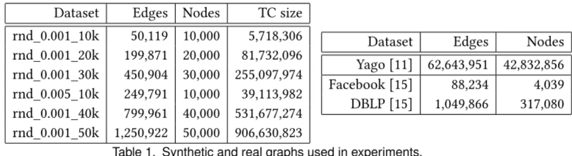
Dataset Edges Nodes TC size rnd_0.001_10k 50,119 10,000 5,718,306 rnd_0.001_20k 199,871 20,000 81,732,096 rnd_0.001_30k 450,904 30,000 255,097,974 rnd_0.005_10k 249,791 10,000 39,113,982 rnd_0.001_40k 799,961 40,000 531,677,274 rnd_0.001_50k 1,250,922 50,000 906,630,823
Dataset Edges Nodes Yago [11] 62,643,951 42,832,856 Facebook [15] 88,234 4,039 DBLP [15] 1,049,866 317,080
Table 1. Synthetic and real graphs used in experiments.
In addition to the examples of section 2.4, we evaluate two variants of TC and SP: TC filter and SP filter, where we compute the paths starting from a subset of 2000 nodes randomly chosen in the graph.
Datasets. We use two kinds of datasets:
• Real world graphs of different sizes, presented in Table 1, including a knowledge graph (the Yago [11] dataset11), a social network graph (Facebook), and a scientific collaborations network (DBLP) taken from [15].
• Synthetic graphs shown in Table 1, generated using the Erdos Renyi algorithm that, given an integer n and a probability p, generates a graph of n vertices in which two vertices are connected by an edge with a probability p. rnd_p_n denotes such a synthetic graph, whereas rnd_p_n_W denotes a rnd_p_n graph with edges weighted randomly (between 0 and 5). Other synthetic graphs are:
– flight_p_n: where edges are taken from rnd_p_n with random depart and arrival times and duration assigned to them.
– c_p_n: serialized object RDD files representing paths between cities. It is also generated from rnd_p_n, each city has been assigned up to 10 random landmarks.
– u_n: serialized object RDD files of n users, each assigned up to 15 random movies. Experimental setup. Experiments have been conducted on a Spark cluster composed of 5 machines (hence using 5 workers, one on each machine, and the driver on one of them)12.
For the Yago dataset, transitive closures are computed for the isLocatedIn edge label. The hand written spark program (manual-spark) has the optimizations PF and PA whenever possible, Pdistis
the only rule it does not have. We have also written the DIQL queries in such a way they apply PF. Such a pre-filtering was not possible for Emma because the programs perform a non linear fixpoint. Trying to write a linear version leads to an exception in the execution. We were not able to write an Emma program that computes movie recommendations. Iterating over a users own movies leads to an exception.
Results summary. Figure 5 presents the obtained results. We observe that the programs generated by mu-monoid systematically outperform the other program versions. The speedup is even more important for programs where PA is applied (SP, SP filter and path planning), especially when combined with Pdist.
11We use a cleaned version of the real world dataset Yago 2s [11], that we have preprocessed in order to remove duplicate RDF
[6] triples (of the form <source, label, target>) and keep only triples with existing and valid identifiers. After preprocessing, we obtain a table of Yago facts with 83 predicates and 62,643,951 rows (graph edges).
12Each machine has 40 GB of RAM, 2 Intel Xeon E5-2630 v4 CPUs (2.20 GHz, 20 cores each) and 66 TB of 7200 RPM hard
Fig. 5. Compar ison of prog ram running times (repor ted in seconds on the y-ax es). A bar reaching the maximal v alue on the y-axis indicates a timeout.
This experimental comparison shows the benefit of the plan that distributes the fixpoint. It also highlights the benefits of the approach that synthesises code: generating programs that are not natural for a programmer to write, like the distributed loop to compute the fixpoint.
5 RELATED WORKS
Bigdata frameworks such as Spark and Flink offer an API with operations (such as map and reduce) that can be seen as a highly embedded domain specific language (EDSL). As explained in [3], this API approach (as well as that of other EDSLs) offers a big advantage over approaches like relational query languages and Datalog as they allow to express (1) more general purpose computations on (2) more complex data in their native format (which can be arbitrarily nested). Also, functions such as map and reduce can have as argument any function f of the host language13(called second order functions map f and reduce f) thus exposing parallelism while allowing a seamless integration with the host language. However, as pointed out by [3], this approach suffers from the difficulty of automatically optimizing programs. To enable automatic optimizations, they propose an algebra based on monads and monad comprehensions and propose an EDSL called Emma. Emma targets JVM-based parallel dataflow engines (such as Spark and Flink). However, in order to support recursive programs (a large class of programs), one needs to use loops to mimick fixpoints but optimizations are not available for such constructs.
LINQ [17] and Ferry [13] are other comprehension based languages. However, unlike Emma, they do not analyse comprehensions to make optimizations. Moreover, as they target relational database management systems (RDBMS), the set of host language expressions that can be used in query clauses like selection and projection is restricted. A complete survey of those works and of other EDSLs can be found in [3]. The support of recursive query optimization in RDBMS has been recently substantially improved in [14]. However, [14] is restricted to the centralized setting, and to relational algebra. Datalog, another recursive query language has been studied in the distributed setting in [20]. These lines of works focus only on modeling data access (with no or poor support for user-defined functions for instance), not general computations such as in more complete programming languages.
The authors of [1] trace the effort of using monads back to Buneman who showed in [4] that the so-called monads can be used to generalize nested relational algebra to different types of collections and complex objects. The idea of using monoids and monoid homomorphisms for modeling computations with data collections can be even found earlier in the works of [21, 22]. It can also be found in the concepts of on list comprehensions [19, 23], monad comprehensions [24], ringad comprehensions [12].
The work found in [8] is pursuing a similar goal to that of Emma, which is to optimize EDSLs that express distributed computations. He proposed an algebra based on monoid homomorphisms therefore with parallelism at its core: an homomorphic operation H on a collection is defined as the application of H on each subpart of the collection, results are then gathered using an associative operator. Distributed collections are modelled using the union representation of bags, and collection elements can be of any type defined in the host language. The authors designed DIQL [10] (a DSL that translates to the monoid algebra). Using reflection of the host language (Scala in this work) and quotations, queries of this DSL can be compiled and type checked seamlessly with the rest of the host language code. In fact, Emma uses the same approach as well.
Fegaras proposed a monoid comprehension calculus first [9] which later evolved in the monoid algebra presented in [8]. The algebra of [8] has a repeat operator which suffers from the same limitations as Emma [3] : no optimization technique is provided.
In this work, we show that having a fixpoint as a first class operator in the algebra (which can be seen as a fold operation in the monad formalism) introduce even further optimization opportunities, integrates well with the other operators and offers a considerable gain in performance in practice.
6 CONCLUSION
We propose to extend the monoid algebra with a fixpoint operator that models recursion. The extended µ-monoids algebra is suitable for modeling recursive computations with distributed data collections such as the ones found in big data frameworks. The major interest of the “µ” fixpoint operator is that, under prerequisites that are often met in practice, it can be considered as a monoid homomorphism and thus can be evaluated by parallel loops with one final merge rather than by a global loop requiring network overhead after each iteration.
We also propose rewriting rules for optimizing fixpoint terms: we show when and how filters can be pushed into fixpoints. In particular, we find a sufficient condition on the repeatedly evaluated term (φ) regardless of its shape, and we present a method using polymorphic types and a type system such as Scala’s to check whether this condition holds. We also propose a rule to prefilter a fixpoint before a join. The third rule allows for pushing aggregation functions inside a fixpoint.
Experiments suggest that: (i) Spark programs generated by the systematic application of these optimizations can be radically different from – and less intuitive – than the input ones written by the programmer; (ii) generated programs can be significantly more efficient. This illustrates the interest of developing optimizing compilers for programming with big data frameworks.
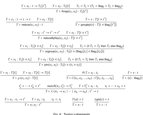
A WELL-TYPED TERMS
We define typing rules for algebraic terms, in order to exclude meaningless terms. In these rules, we use type environmentsΓ which bind variables to types. An environment contains at most one binding for a given variable. We combine them in two different ways:
• Γ ∪ Γ′is only defined ifΓ and Γ′have no variable in common, and is the union of all bindings inΓ and Γ′;
• Γ + Γ′is defined by taking all bindings inΓ′plus all bindings inΓ for variables not appearing inΓ′. In other words, if a variable appears in both, the binding inΓ′overrides the one inΓ. Definition A.1 (matching). We first define the environment obtained by matching a data type to a pattern by the following:
match(a, t ) → a : t ∀i match(πi, ti) → Γi
match(C(π1, ..., πn),C[t1, ..., tn]) → Γ1∪ ··· ∪Γn
If, according to these rules, there is noΓ such that match(π, t ) → Γ holds, we say that pattern π is incompatible with type t . Note that, with our conditions, a pattern containing several occurrences of the same variable is not compatible with any type and hence cannot appear in a well-typed term, as the typing rules will show.
Definition A.2 (operation+ and relation <: on sum types). The operation + on sum types is defined recursively as follows. Let t be a sum type and C a constructor not appearing in t , then:
t+ (t1′|| ··· ||tm′ ) = (t + t1′) + (t ′ 2|| ··· ||t ′ m) t+ C[t1, ..., tn]= t || C[t1, ..., tn] (t || C[t1, ..., tn]) + C[t1′, ..., tn′]= t || C[t1+ t1′, ..., tn+ tn′]
The type t + t′is not defined if t or t′is not a sum type, or if they have constructors in common with incompatible type parameters, i. e. type parameters which cannot themselves be combined with+.
Γ ⊢ e1: t → T1[t′] Γ ⊢ e2: T2[t ] T1= T2∨(T1=Bagl∧T2=Bagd) Γ ⊢flmap(e1, e2) : T2[t′] Γ ⊢ e1: t → t → t Γ ⊢ e2: T [t ] Γ ⊢reduce(e1, e2) : t Γ ⊢ e : T [t × t′ ] Γ ⊢groupby(e) : T [t ×Bagl[t′]] Γ ⊢ e1: t′→t′→t′ Γ ⊢ e2: T [t × t′]
Γ ⊢reduceByKey(e1, e2) : T [t × t′]
Γ ⊢ e1: T1[t × t1] Γ ⊢ e2: T2[t × t2] T3= (ifT1= T2 thenT1 else Bagd) Γ ⊢cogroup(e1, e2) : T3[t × (Bagl[t1] ×Bagl[t2])]
Γ ⊢ e1: T1[t × t1] Γ ⊢ e2: T2[t × t2] T3= (ifT1= T2 thenT1 else Bagd) Γ ⊢join(e1, e2) : T3[t × (t1×t2)] Γ ⊢ e1: T [t ] Γ ⊢ e2: T [t ] → T [t ] Γ ⊢ µ (e1, e2) : T [t] ∀iΓ ⊢ ei : ti Γ ⊢ C(e1, e2, ..., en) : C[t1, t2, ..., tn] Γ ⊢ e : t Γ ⊢ {e} :Bagl[t ] t1′+ ··· + tn′ = t′ match(πi, ti′) → Γi′ Γ + Γi′⊢ei : ti t1+ ··· + tn = t Γ ⊢ λ (π1→e1| ··· |πn→en) : t′→t Γ ⊢ e1: t1→t′ Γ ⊢ e2: t2 t2<: t1 Γ ⊢ e1e2: t′ Γ(a) = t Γ ⊢ a : t type(c) = t Γ ⊢ c : t
Fig. 6. Typing judgements.
Definition A.3 (Well-typed terms). A term e is well-typed in a given environmentΓ iff Γ ⊢ e : τ for some type t , as judged by the relation defined in Figure 6. In these rules, T represents one of
Bagl orBagd.
Note that these rules do not give a way to infer the parameter type of a λ expression in general; we assume some mechanism for that in the language L. An interesting particular case, however, is when a λ expression is used directly as the first parameter of aflmap(, ) orreduce(, ). We can write
the following compound deterministic rule in the case offlmap(, ), for example:
Γ ⊢ e2: T2[t ] match(π, t ) → Γ′ Γ + Γ′⊢e1: T1[t′] T1= T2∨(T1=Bagl∧T2=Bagd) Γ ⊢flmap(λ (π → e1), e2) : T2[t′]
B ADDITIONAL PROOFS
In the following, we suppose (fc): ∀A, B φ(A ⊎ B) = φ(A) ⊎ φ(B)
B.1 Proving the existence of the fixpoint
We have ψ = R ⊎ φ
We prove that the fixpoint of f : X → X ∪ ψ(X ) exists: We consider the following bag F = Un ∈Nφ(n)(R) We have φ(F ) = φ(Un ∈Nφ(n)(R)) = Un ∈Nφ(n+1)(R) (fc)