Chromatic dispersion compensation using a Virtually Imaged Phased Array (VIPA)

Chromatic Dispersion Compensation Using a

Virtually Imaged Phased Array (VIPA)

by Christopher Lin

Submitted to the Department of Electrical Engineering and Computer Science in partial fulfillment of the requirements of the degree of

Master of Engineering in Electrical Engineering at the

MASSACHUSETTS INSTITUTE OF TECHNOLOGY June 2000

© 2000 Massachusetts Institute of Technology All rights reserved.

Signature of A uthor... ...-- . ... .

--Department of Electricag-Ergniernng and Computer Science May 12, 2000

Certified by...- . .... ...---. ...-.---...

Hermann A. Haus Institute Professor of Electrical Engineering Thesis Supervisor

Accepted by... .... ...

Arthur C. .th Chairman, Department Committee on Graduate Student

MASSACHUSETTS INSTITUTE

OF TECHNOLOGY

ER

[7771771BARKE

JUL 11

2001

Virtually Imaged Phased Array (VIPA)

by

Christopher Lin

Submitted to the Department of Electrical Engineering and Computer Science on May 12, 2000 in partial fulfillment of the requirements for the degree of

Master of Engineering in Electrical Engineering

Abstract

Chromatic dispersion limits the performance of modem optical communications systems. Chro-matic dispersion causes pulse broadening over long transmission distances, which constrains the bit-rate.

A Virtually Imaged Phased Array (VIPA) in conjunction with a lens and mirror compensates for distortion induced by chromatic dispersion. The VIPA compensator processes all wavelength-division-multiplexed channels in a fiber in parallel. A VIPA is generated from multiple reflections within an etalon that is partially transmissive on one surface and perfectly reflective on the other (aside from an anti-reflection coated input/output window). The virtual images interfere to pro-duce angular dispersion, which is converted to chromatic dispersion by a lens and mirror.

This thesis uses numerical simulation to explore and evaluate the performance of different VIPA compensator configurations. Results demonstrate that the system mirror can be designed to cor-rect arbitrary chromatic dispersion, and that insertion loss is independent of dispersion bias, though mode-shaping through etalon transmissive coating design can permit wide bandwidth and low insertion loss systems.

Thesis Advisor: Hermann A. Haus Title: Institute Professor

Acknowledgements

I would like to thank Dr. Masataka Shirasaki for everything he has shared with me. He always assumed the best in me and always challenged me to solve problems armed with only my wits and a piece of chalk. Above all, he taught me how to use what I already know to answer my own ques-tions.

Being in Professor Hermann A. Haus's company was a pure pleasure. I will forever be amazed at his ability to comprehend anything nearly instantaneously. He always has questions to ask. He showed me that true understanding is the ability to ask questions. I thank him for teaching me how to ask my own questions and for the opportunity to work with him.

I thank Patrick Chou, Juliet T. Gopinath, and Jeremy D. Sher for taking the time to help me with my thesis presentation and text. I also thank Afsana N. Akhter, with whom I worked last year, for being a great co-worker and for paving the way for my own thesis.

I thank Dr. Simon Cao, Dr. Charlene Yang, and Jay Ma for fruitful discussions and insights. I also thank the members of the Optics and Devices Group for their wonderful weekly presentations.

Finally, I extend my heartfelt thanks to my family, friends, and teachers who have taught me so much and made my life so joyful.

List of Figures... 6 List of Tables...8 1.0 Introduction... 19 1.1 Current technology... 11 1.2 VIPA description...11 1.3 Design considerations... 14 2.0 Theoretical Dispersion... 19 3.0 M irror Design...22 3.1 Parabolic mirror... 22

3.2 Constant dispersion mirror...22

3.3 Arbitrary dispersion mirrors... 24

4.0 Num erical M odel... 27

4.1 Parameters... 27

4.2 Inside the etalon... 27

4.3 Lens and mirror... 31

5.0 Sim ulation Results ... 35

5.1 Constant transmissivity... 36

5.2 Linear transmissivity...41

5.3 M ulti-level transmissivity... 45

5.4 Constrained coating comparison... 52

6.0 Finer Points... 56

6.1 Predicting center wavelength... 56

6.2 Transmission spectrum clipping at

E

= 2.8 ... 58

6.3 Secondary-lobe cross-talk... 59

6.4 M ismatched constant dispersion mirror... 60

6.5 Thickness mismatch in 2-level transmissivity coating... 62

6.6 M ode width wavelength dependence... 64

7.0 Conclusions... 65

References...66

Appendix A: Experim ental Corroboration... 67

Appendix B: Application to Polarization Mode Dispersion... 69

Figure 1-1: Schem atic of VIPA com pensator... 10

Figure 1-2: Virtually imaged phased array generation... 12

Figure 1-3: Light paths for different wavelengths... 13

Fig u re 1-4 : In itia l w in d o w lo ss...16

Figure 2-1: Transm ission angle in etalon ($)... . 19

Fig u re 2 -2 : Lig h t p a th ... 2 0 Figure 2-3: Light paths of complementary virtual images... 21

Figure 3-1: Shape of two constant dispersion mirrors (K=45,70)... 23

Fig ure 3-2: Line a r d isp e rsio n m irro r... . 26

Figure 4-1: Reflections at etalon transmissive surface... 30

Figure 4-2: Lobes of VTOta in the focal plane... 31

Figure 4-3: Illustration of the power center of TMain-..--.---... ... ...-... 33

Figure 4-4: Focusing -lens a lig nm ent... 33

Figure 5-1: 2.0 % transmissivity, r = 3 cm parabolic mirror... 38

Figure 5-2: 2.0 % transmissivity, K = 70 constant dispersion mirror...38

Figure 5-3: 1.5 % tra nsmissivity, r = 3 cm parabolic mirror... 39

Figure 5-4: 2.5 % transmissivity, r = 3 cm parabolic mirror... 39

Figure 5-5: 2.0 % trans., r = 3 cm, trans. and refl. modes (E = 2.50)...40

Figure 5-6: 2.0 % trans., r = 3 cm, dispersion derivation (E = 2.50)...40

Figure 5-7: 40%/cm transmissivity, r = 3 cm parabolic mirror...42

Figure 5-8: 40%/cm transmissivity, K = 70 constant dispersion mirror... 42

Figure 5-9: Varied linear transmissivity, r = 3 cm parabolic mirror...43

Figure 5-10: Varied linear transmissivity, K = 70 and K = 45 constant dispersion mirror...43

Figure 5-11: 40%/cm trans., K = 70, trans. and refl. modes (E = 2.50)...44

Figure 5-14: Varied slope 2-level transmissivity, r =3 cm parabolic mirror...47

Figure 5-15: Varied slope 2-level transmissivity, K = 70 constant dispersion mirror...47

Figure 5-16: Varied slope 2-level transmissivity, K = 45 constant dispersion mirror...48

Figure 5-17: 20%/cm 2-level trans., K = 70, trans. and refl. modes (0 = 2.50)...48

Figure 5-18: Varied slope 3-level transmissivity, r = 3 cm parabolic mirror...50

Figure 5-19: Varied slope 3-level transmissivity, K = 70 constant dispersion mirror...50

Figure 5-20: Varied slope 3-level transmissivity, K = 45 constant dispersion mirror...51

Figure 5-21: 20%/cm 3-level trans., K = 70, trans. and refl. modes (0 = 2.50)...51

Figure 5-22: C onstrained coating com parison... 52

Figure 5-23: Tunable dispersion variation for parabolic mirror... 54

Figure 5-24: Tunable dispersion variation for constant dispersion mirror... 55

Figure 6-1: VIPA G aussian beam idealization... 56

Figure 6-2: Far-field envelope and m odulation... 57

Figure 6-3: Transmission spectrum clipping at E = 2.8 ... 58

Figure 6-4: Secondary-lobes for E = 2.50 and 2.80 ... 59

Figure 6-5: Secondary-lobe cross-talk... 59

Figure 6-6: Mismatched constant dispersion mirror...60

Figure 6-7: Simplified 2-level trans. and refl. modes with thickness-mismatch...62

Figure 6-8: Simplified and numerical effects of thickness-mismatch...63

Figure 6-9: Ray spacing dependence on wavelength... 64

Table 3-1: Coefficients of mirror shape, c(y)...25

Table 3-2: Linear dispersion mirror coefficients...26

Ta b le 4 -1: List o f p a ra m e te rs...2 7 Table 5-1: Constant transmissivity scenarios... 37

Ta ble 5-2: Linea r tra nsm issivity scenarios... 41

Table 5-3: 2-level transm issivity scenarios... 46

Table 5-4: Level values and junction locations for 2-level transmissivity... 46

Table 5-5: 3-level transmissivity scenarios... 49

Table 5-6: Level values and junction locations for 3-level transmissivity... 49

Table 5-7: Constrained coating comparison...53

Table 5-8: Tunable compensator (r = 3 cm)... 54

Table 5-9: Tunable compensator (K = 70)... 55

Table 6-1: Mismatched constant dispersion mirror... 61

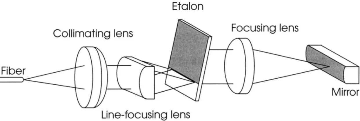
Collimating lens Focusing lens

Fiber

Mirror Line-focusing lens

Figure 1-1: Schematic of VIPA compensator

1.0 Introduction

Chromatic dispersion in optical fibers limits the bandwidth or transmission distance of

high performance communications systems. Chromatic dispersion arises from the physical reality

that different wavelengths travel at different group velocities through an optical fiber. Although

this effect is small, the resultant pulse broadening becomes substantial over long distances or at

high bit-rates. Pulses that will spread need to be spaced farther apart than pulses that will not

spread, to avoid pulse overlap and subsequent detection errors. Greater space between pulses

translates to lower bit-rate. A Virtually Imaged Phased Array (VIPA)' provides a low loss,

com-pact, and tunable solution to the problem of chromatic dispersion compensation [1,2]. The VIPA

compensator also simultaneously processes all wavelength-division-multiplexed channels in an

1.1 Current technology

The conventional method of compensating for chromatic dispersion is to use Dispersion Compensating Fiber (DCF) [3]. Standard optical fibers have positive dispersion, whereas DCF has negative dispersion. However, the length of DCF needed to compensate a given amount of chromatic dispersion is comparable to the length of the fiber generating the chromatic dispersion, on the order of 25 km of DCF per 100 km of standard single-mode fiber. This large length of DCF eliminates the possibility of a compact compensator. In addition, DCF is lossy and introduces its own distortion through a large nonlinear effect, due to its narrow core size. Finally, DCF is not tunable, which hampers the flexibility of systems incorporating such fibers. A VIPA based system can produce large, tunable chromatic dispersion with low loss and no nonlinear effects in a com-pact module.

Alternative technologies based on diffraction gratings or Bragg grating filters [4] have other limitations. Diffraction gratings with enough angular dispersion to be useful have polariza-tion dependent loss. Bragg grating filters provide chromatic dispersion only in discrete steps. They are also very long, on the order of tens of meters. A compensator built with a VIPA has no polarization dependent loss and provides continuous dispersion over wavelength.

1.2 VIPA description

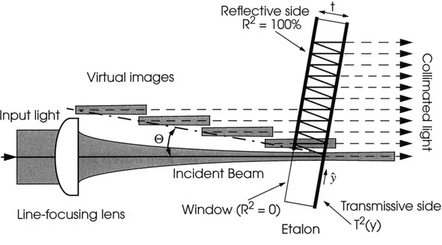
A VIPA is generated by an etalon, made of air or glass, with reflection coatings on both sides. The reflective side has a 100% reflection coating except for an input/output window which is anti-reflection coated. The transmissive side is only partially reflective with a coating that can have an arbitrary functional form (this research considers constant, linear amplitude (parabolic intensity), and multi-level transmissivity profiles).

R2= 100%

--- ₀

Virtual images =

Input light--...a asmsa - - - - -- - - - .

Incident Beam

Line-focusing lens Window (R2 = 0) Transmissive side

Etalon T2_(y)

Figure 1-2: Virtually imaged phased array generation

The input is a Gaussian beam from a single-mode optical fiber. This light is first allowed to

diverge and is then collimated using a spherical lens. It is then line focused, through a

semi-cylin-drical lens, into the VIPA plate. The etalon is tilted at an angle

E

so that the multiple reflections

within the etalon create an array of virtual images that interfere on the etalon's transmissive

sur-face (see FIGURE 1-2). Notably, these virtual images are in phase since they all originate from the same initial image. This fact is central to determining the wavelength dependent transmission

angle (D (presented in SECTION 2).

A lens and mirror complete the system. The lens transforms the etalon's angular

disper-sion into a lateral translation in the focusing lens's focal plane, where the mirror is placed. The

reflection from a flat mirror back through the lens and onto the etalon's transmissive surface is

flipped and shifted. The shift depends on the initial angular dispersion, which is dependent on

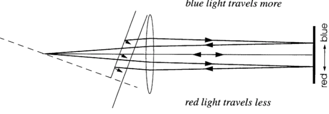
blue light travels more

red light travels less

Figure 1-3: Light paths for different wavelengths

deflected upwards and is reflected farther up the etalon. In order to exit the etalon through the win-dow and return to the optical fiber, it must bounce back and forth between the etalon's mirrors more times than red light; it therefore encounters a longer path length (see FIGURE 1-3).2 By

changing the shape of the mirror, this basic effect can be magnified. By changing the detailed pro-file of the mirror, the functional form or shape of the dispersion can be modified. Finally, by changing the distance between the etalon and lens (and keeping the lens-mirror spacing fixed), the dispersion can be tuned.

The etalon can be thought of as a mode transformer. It takes the mode of an optical fiber (a Gaussian beam) and transforms it into some transmission mode on its transmissive surface. The lens and mirror merely feed a modified version of this transmission mode back into the etalon. By reversing the operation of the etalon, the ideal mode that would produce a Gaussian beam at the optical fiber can be defined. With this definition, the integral of the overlap between the reflection

mode and the ideal mode yields the coupling loss of the modes as well as the group delay. The

2. The ray trace in FIGURE 1-3 only shows what happens to the virtual image source along the lens axis. As

will be shown in SECTION 2, the light path is independent of the initial virtual image. Therefore, following only one image completely describes the compensator's operation.

conjugate of the transmission mode. Since the dispersion comes from the shift of the reflection mode relative to the ideal mode, greater shift means more loss since the overlap integral is smaller if the two modes are spaced farther apart.

A VIPA can also be used to perform wavelength division multiplexing/de-multiplexing. References [5]-[7] describe this function and provide relevant insight into the chromatic disper-sion compensation application.

1.3 Design considerations

Seven variables determine the performance specifications of the VIPA chromatic disper-sion compensator. These are the input beam waist wo, the input angle (E in air and 0 in etalon),

the etalon's thickness t, the etalon's index of refraction n, the width of the transmission mode (related to the transmissivity profile of the etalon's transmissive surface T(y)), the focal length of

the lens

f,

_{and the shape of the mirror c(y). These variables determine the dispersion bias,}3 _the shape of the dispersion profile, the insertion loss, the bandwidth, and the free spectral range (FSR) of the VIPA compensator.

Of these five performance specifications, two involve no substantial trade-offs: dispersion shape and FSR. Shaping the dispersion profile by changing c(y) will not greatly affect the band-width as long as the dispersion bias is unchanged. The bandband-width may be improved or degraded depending on whether the dispersion at the band edges is decreased or increased respectively.

3. In general, the dispersion generated by the VIPA compensator will not be constant over wavelength. In

order to provide a useful reference for comparison between different VIPA compensator configurations, dispersion bias has been defined as the dispersion at the center wavelength of the center WDM channel. Furthermore, the center wavelength is defined as the wavelength in the center of the -1 dB band. This

Since the FSR is set by industry standard (100 GHz or 0.8 nm), the values of t and n must be cho-sen to ensure that the transmission angles of wavelengths differing by an integer multiple of the

FSR are identical (see SECTION 2).

The index of refraction is the overall performance limiting factor. The etalon thickness and index of refraction determine the FSR, but larger n greatly increases the potency of the compensa-tor. As will be seen in SECTION 2, the compensator's dispersive ability is proportional to the fourth power of the etalon's index of refraction.

Having discussed the dispersion shape and FSR, there are only three fundamental metrics left to consider: insertion loss, bandwidth, and dispersion bias. In fact, the only trade-off will be between bandwidth and dispersion. As will be shown, the insertion loss is independent of both. Herein lies perhaps the most important advantage of the VIPA compensator over DCF. The loss (in dB) of DCF increases linearly with dispersion. For large amounts of dispersion, the VIPA compensator will undoubtedly have less loss than DCF. The price for this freedom is bandwidth narrowing. DCF has no bandwidth limitations. The transmission spectrum of DCF over a single WDM channel is completely flat.

Characteristic waist wo

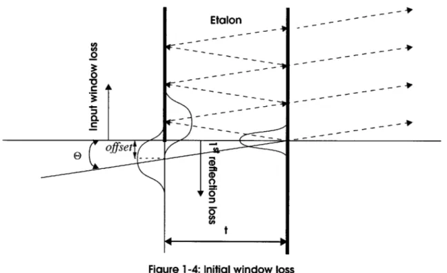
The input to the VIPA compensator is assumed to be the output of a single-mode optical fiber. The amplitude profile can be approximated by a Gaussian. To a first-order approximation, the input window loss is minimized when the beam is line-focused onto the transmissive surface of the etalon along the same line where the highly reflective coating is applied on the reflective surface (see FIGURE 1-4). Any other point of focus will increase the input window loss or first reflection loss by more than it reduces the other.

0

o et

Figure 1-4: Initial window loss

The waist that minimizes the initial window loss at the undeflected wavelength is the most narrow waist at the etalon's reflective surface (see EQUATION 1.1). The beam waist of the power profile is equal to this value divided by 12. Using trigonometry, the offset can be computed from the refractive index adjusted incident angle 0 in the etalon. This offset is the distance between the beam center and the reflective surface coating discontinuity. All of the power that falls above the coating is lost.

Minimal window loss characteristic waist computation

2 2;[ nrfI] [11 2 2 dw 2X, Z = 2w0- 2 2 = 0 d 0 0 0n CA (A

Estimated window loss4

offset = t - tanO

offset

- erf _.

Kpow e rWa ist)

windowLoss =2 [1.2]

Input angle

E

Smaller incident angles increase the dispersion bias but also increase the window and eta-lon losses, since more initial power is cut off and more power can escape during subsequent reflections. The bandwidth also decreases with decreasing angle of incidence since larger disper-sion means the reflected mode is displaced farther from the ideal mode and therefore does not couple as well.

Transmission profile T(y)

The transmission profile shapes the VIPA modes (transmission and reflection). Wider modes overlap better at the band edges (higher bandwidth), but sacrifice dispersion bias (see SEC-TION 2). The presence of non-centralized peaks in the mode profile enhances bandwidth, and sym-metric modes have lower insertion loss than asymsym-metric modes.

Focal length f and mirror shape c(y)

The focusing lens converts the VIPA's angular dispersion into chromatic dispersion by mapping the different etalon transmission angles to different positions in the focal plane where the mirror is located, and therefore to different traveling distances. Largerf or smaller radius of curva-ture results in higher dispersion but lower bandwidth, since the displacement between the reflec-tion mode and the ideal mode will increase more rapidly over wavelength with largerf or smaller radius of curvature.

In addition to providing a quantitative way of evaluating insertion loss, bandwidth, and dispersion, this thesis provides insight into engineering the shape of the VIPA mirror. The VIPA chromatic dispersion compensator tends to produce greater negative dispersion for longer wave-lengths. This trend may or may not have anything to do with the dispersion to be compensated. To be truly useful, there must be an easy way to design a mirror to produce a compensation profile that is matched to the particular application. In the tunable case, this mirror shape will have to be a compromise over the range of operation unless the mirror can also be tuned.

One final consideration is the deviation of compensation of the system for different chan-nels. The VIPA is optimized for the center channel in a WDM band. Other channels have slightly different wavelengths and therefore react differently to the various components of the VIPA com-pensator. Other channels also have different dispersion. The VIPA compensator corrects each channel in the same way. All channels are improved, but only the center channel is completely compensated.

2.0 Theoretical Dispersion

While the insertion loss of the VIPA compensator is hard to predict analytically, the dis-persion performance can be readily described using straightforward ray optics.

mnl/n

2t

Figure 2-1: Transmission angle in etalon ($)

As mentioned in SECTION 1.2, the virtual image sources of the VIPA are all in phase. This reduces the calculation of the wavelength dependent transmission angle to an antenna problem. The differential path length between two sources must be an integer multiple of the index adjusted wavelength in order to have constructive interference:

(D n$, cos$ = MX >n [2.1]

The FSR is also implicitly contained in EQUATION 2.1. When X is varied by an integer

mul-tiple of the FSR, D must remain constant. Therefore, (m - k)(Xm + k - FSR) where k is some

integer must stay fairly constant as k is varied over the integers. This constrains the value of nt, since nt determines m when (D, Xm, and the FSR are fixed.

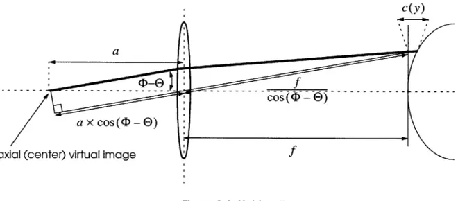
The light path from the virtual image along the lens axis to the mirror and back can be approximated by EQUATION 2.2, where a is the distance between the axial or center virtual image and the lens, and c(y) is the shape of the mirror (see FIGURE 2-2). FIGURE 2-2 is somewhat

mis-ab

cos(D -E) a x cos((D -E))

axial (center) virtual image f

Figure 2-2: Light path

leading because the angle (c-E) is too small to be accurately depicted. In the limit where (c-e) is very small:

lightPath = 2 a - cos( -E) +

)+

c(y)] [2.2]

L cos((D - E))

y =

f((D-E))

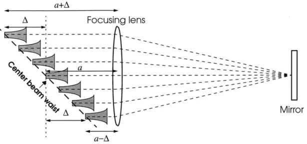
The system geometry demonstrates that this light path applies to all light of a specific wavelength from each of the virtual images. FIGURE 2-3 shows the undeflected case, but the result is general. The optical paths to the right of the lens are all equal because of the effect of the lens, and the optical paths to the left of the lens are equal because the sum of the distances between any complementary pair of images and the lens is always 2a.

The phase advance for each wavelength is:

phaseChange = lightPath

~ 2 ( 2

a+A

A Focusing lens

a-A

Figure 2-3: Light paths of complementary virtual images The derivative of y with respect to o yields the group delay:5

groupDel

G

-2X[( G=C( dy =G = -dw ay -X 2 dy 2ncdX

f

a)(D- E))+ h(y)dY d(D

d h(y) = d c(y)

dy 2

G =I (f - a)((D - E) +

fh(y)

}

[2.4]

Finally, the derivative of the group delay with respect to wavelength is the dispersion:

dispersion = D = dG

dA _cX(D3I 2n

[3(f

- a)F +f 24Jd h(y) _dyI - fh(y)]

This expression explains why wider transmission modes have lower dispersion. Wider modes are centered farther up the etalon. This increases the value of a which decreases the

magni-tude of the dispersion. Also, the dispersion is proportional to n4, which calls for high-n etalons.

5. The first term is ignored since it is roughly constant over the WDM channel and only the change in group delay is important (see APPENDIX B).

0

-A a NO !-

---irror

M [2.5] --- 7

The mirror placed in the focal plane of the focusing lens has a profound effect on the dis-persion produced by the VIPA compensator. Placing a convex mirror, for example a simple para-bolic mirror, in the focal plane will augment the overall dispersive effect. More complicated mirrors can shape the dispersion as a function of wavelength. For example, the natural tendency of the VIPA is for longer wavelengths to have greater dispersion. The correct mirror can cancel this tendency and provide constant dispersion over the range of operation.

3.1 Parabolic mirror

For a parabolic mirror, EQUATION 2.5 yields:

2

c(y) = Y 2r

D = - n(f-a)+f}

cX(D3 r

This dispersion can vary over a 0.6 nm band by nearly an order of magnitude.

3.2 Constant dispersion mirror

A more interesting case is uniform dispersion over the WDM channel. Since X changes very slowly over the band, the dispersion will be very uniform if the multiplicand in brackets in

EQUATION 2.5 is proportional to D3.

2d 3 2n4K0

(f - a)D + f 2 DI- h(y) - fh(y) = K= Do 2 4 K

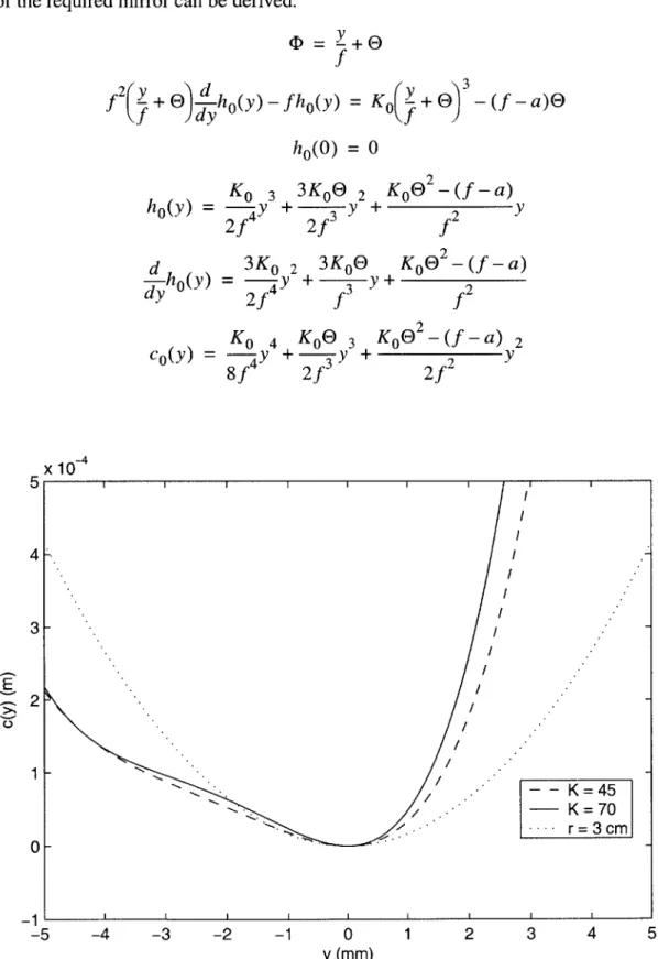
By assigning the initial condition h(O) = 0 and solving this differential equation in y, the shape of the required mirror can be derived:

D

f

E+

f

f 2r1+0

_'f)

_dy

'h 0(y)- fh(y) = -(f -a)9 ho(O) = 0

K0 3 3KOE 2 KO)2 - (f -a)

ho(y) 4y + Ty + 2 7

2f 2f f

2

d hO(Y) = 3K2 3KOE K₀ -(f-a)

d

2f

f

f

2 cO(y) = K 4 8f K0E 3 + 3y 2f -4 -3 -2 -1 0 y (mm) 2 K0 -(f -a) 2 2f 2 1 2 3 4 5

Figure 3-1: Shape of two constant dispersion mirrors (K=45, 70)

x 10 5 4 3

E

2 1 0 -I -. /. - --/ K=45 -- K =70 ..-. _{r = 3cm} -5 Ko( + E) i i i i i j I I

More complicated mirrors can produce arbitrary dispersion profiles. The process is indi-rect since the mirror shape is most easily described as a function of y which is proportional to

JX.

The basic method of computing these mirror shapes as a function of y begins with assuming a pro-portionality relationship, as in the previous section for the constant dispersion case. Here, a few of the lower-order cases are presented.

First-order mirror (f-a)D+f 2 h(y)-fh(y) = K y -> DI 2n Ky dy cx KI 4 5K ₁e 3 hI(y)= -y+ ₃ y+ 3f 6f K1 5 5K 1 4 y 4y + 3 y + 15f 24f KI E)2 227 2f 2 2 3 6f2 Second-order mirror 2d 3 2 (f -a)D+f 2 h(y)-fh(y) = K20 y dy 4 2 2n K2y cx h2(y) = K₂ 5 + c2(y) = K~ 6 4fy + 24f 7K₂E 4 K20 3 Sy + 2 ' 12f 3f 7K_{2E5 K2E 24} 3 y+ 2-60f 12f Third-order mirror 2

d3

3 (f -a) +f - h(y)-fh(y) = K3c y -dy K3 6 9K3E 5 K3E2 4 h3(y)= y + 3 y + 2 Y

5f

20f

4f

K3 7 3K3E 6 K3

9

2

5

c3(y) = gy + y + 2 35f 40f 20f 2n 4K3y3 = cX

Fourth-order mirror

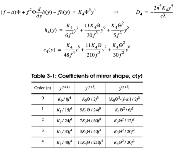
(f -a) +f 2D+h(y)- fh(y) = K43 y

-dy K4 7 lIK4 6 K462 5 h4(y)= -- y + 3 y+ 27" 6f 30f

5f

K₄ 8 lIK40 7 K42 6 48f 210f 30f 2n4K4y4 D4 =

-Table 3-1: Coefficients of mirror shape, c(y)

Order (n) y(n+4) y(n+3) y(n+2)

0 K₀ / 84 K₀E/ 2f [K0e2-(f-a)] / 2j2

1 K₁ / 15fi 5K₁ E/ 24f K1E2 / 6j

2 K2 / 244 7K2E/ 60f K2E2 / 12f

3 K3 / 35f 3K3E/ 40f K3E2 / 20#

4 K₄/ 48f 11K ₄E/ 210f K4E2 / 302

The most straightforward way to use these equations is to map the desired dispersion as a function of wavelength to the desired dispersion as a function of y. Then, a linear least squares

superposition of these mirrors would yield the desired profile.

(- 2 tx '2 22nt

y=f(Q-e)

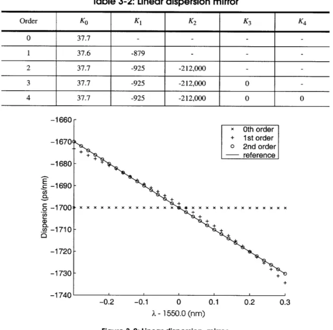
y=f n 2- -O=n 2-nt cos(Tn =

ps/nm at 1550.0 nm with a slope of -100 ps/nm2. TABLE 3-2 lists the K, coefficients for succes-sively higher orders of linear least squares approximations to the reference line. FIGURE 3-2 plots

the results. In this particular example, the 3rd and 4th order terms are not needed.6

Table 3-2: Linear dispersion mirror

Order K0 K1 K2 K3 K4 0 37.7 - -1 37.6 -879 -2 37.7 -925 -212,000 -3 37.7 -925 -212,000 0 4 37.7 -925 -212,000 0 0 -1660 r -1720 -1730 -1740 -0.2 -0.1 x0th order + 1st order o 2nd order + + - reference - + 0 0.1 0.2 0.3 X - 1550.0 (nm)

Figure 3-2: Linear dispersion mirror

6. The dispersion over a single WDM channel is essentially constant. The usefulness of arbitrary dispersion

mirrors turns out to be in so-called "dispersion slope compensators" (also built around a VIPA) which produce different dispersion for different WDM channels. The VIPA compensator discussed in this work

1670( 1680 E C-0 a) 0_ 1690 1700: 1710

4.0 Numerical Model

The VIPA compensator is a simple device. Its dispersion performance is accurately pre-dicted by ray optics. Only basic diffraction-limit optics theory is needed to fully describe the VIPA compensator's operation. Haus's text provides an excellent description of these theoretical tools [8]. For this thesis, this diffraction limit model was programmed using MATLABTM in order to sketch the compensator's transmission spectrum. The simulation also calculated the dispersion performance in order to confirm the ray optics results.

4.1 Parameters

Table 4.1: List of parameters

Parameter Symbol

index of etalon n

etalon thickness t

wavelength in free space X

beam waist wo

incident angle in air, in etalon E, 0

transmission angle in air, in etalon CD, $ focal length of focusing lens f distance between etalon and lens I

distance between center virtual image and lens a

transmission coating T(y)

shape of mirror c(y)

4.2 Inside the etalon

Since the VIPA is operating in the paraxial limit, the Fresnel diffraction integral describes the behavior of the input light within the device. Application of the Fresnel diffraction integral is

u(y, z) = exp(jkgassz)

f

u0(yo)exp zgss(Y -yo) dy

2 U(k,, z) = U0(k,)exp(jkgiassz)exp _{-j2kglass )}

Phase factor forforward propagation:

k 2

phaseFactor = P(z) = exp(jknz)exp Y-jz

Using the phase factor with z = -t on an ideal focused Gaussian beam, with linear phase

offset due to the tilt

E

of the VIPA compensator, the unobstructed input just before the reflective

surface of the etalon can be calculated. If the input light before incidence is normalized, with

nor-malization constant A, the window loss can be computed. The result of the integral must be

squared since power will be lost through this mechanism on the return path as well. Subsequently, the phase factor with z = +t and reflection factors (RL, left or reflective side, and RR, right or

trans-missive side) are repeatedly applied to obtain the complete field profile on the etalon's

transmis-sive surface, TTotal.

Window loss

00 2

windowLoss = 1 -

|

UInitialLeft 2dJ

7. All of the following formulae were implemented using their discrete equivalents. This introduced some

Iterative propagation calculation

U ~-1 F A xp (YY)2 P-)

UInitialLeft = (1 - RL)F F AexP 2 _}P(t)LPhase

0/

LPhase = exp(j(y-y 0 )kgasssin(O))

A =

4

exp (Y - jO) 2 dy UlR = BF~1 {F{ UInitialLeft}PWt) B = IF-1 {F{UInitialLeft}P(t)} 2 dy UIL = F- ({F{RRUlR}Pt)} U2R = F1 ({F{RLUL}P(t)}) N UTotal= EUnR

After enough8 iterations N, the UnR vectors are added to yield the total field profile UTotal

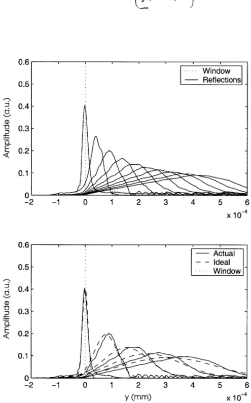
before transmission through the etalon's transmissive surface. This sum is multiplied by T(y), where T(y) is the transmissivity of the transmissive surface, to yield TTotal. Each reflection results

in power loss through the window as well as deviation from the virtual image ideal (see FIGURE

4-1). The total etalon loss is calculated by normalizing the input power after the initial window loss, using normalization constant B, and evaluating the final transmitted power. Again, this result must be squared to account for the return loss by the same mechanism.

8. "Enough" iterations to provide an accurate representation of UTotai in the constant transmissivity case is generally 400. This number depends on the overall transmissiveness of the transmissive coating. A more transmissive coating requires fewer iterations, as light is rapidly lost with each reflection. A less transmis-sive coating requires more.

e o 2

etalonLoss = I -

|IT

Totall 2dy

-1 0 1 2 3 4 5 6

x 10~4

-1 0 1 2 3 4 5 6

y (mm) x

10-Figure 4-1: Reflections at the etalon transmissive surface.

(a) First 10 reflections (2.0 % Transmissivity, E = 2.50). 0.6 0.5 ... Window Reflections -E 0.4-0.3 0.2-0.1 0' -2 0.6 0.5- 0.4- 0.3- 0.2-0.1 aI) E Actual Ideal .... _Window - --1 , 0' -2

4.3 Lens and mirror _0.35

The effect of the lens can be deter- red 10 blue

0.3-mined by first calculating the Fourier trans- Undeflected X form VTotal of TTotal. Given VTotal, VMain for

0.25-the undeflected wavelength is 0.25-the lobe with 2 0.2

the highest power.9 _{For the other wave- -)}

+1

0.15-lengths, VMain is the lobe appropriately

sit0.1 -uated with respect to the undeflected

wavelength's main lobe. VMain for longer 0.05. 1+2

L Ih 1+31+

wavelengths will be the first lobe to the left - 14

0

0 2 4 6

of the undeflected wavelength's main lobe ky (m-1) X 10 5

and VMain for shorter wavelengths will be Figure 4-2: Lobes of VTotaI in the focal plane

the first lobe to the right of the undeflected wavelength's main lobe (see FIGURE 4-2). These main lobes are referred to collectively as the 10 lobes; other lobes have different indices. 10 By first

nor-malizing VTotal, using the constant C, the residual power in VMain and therefore the lobe loss can

be found."1 The inverse Fourier transform of VMain yields TMain, normalized with constant D.

VMain needs to be recalculated from TMain, accounting for lens alignment and phase advance.

9. In general, the undeflected wavelength, defined as the wavelength propagating at CD = E,will not have the least lobe loss. Predicting which wavelength will have the greatest power in its main lobe is impossible without simulation. Because the array of images in the VIPA are not actually ideal Gaussian beams, the profile VTotal cannot be reliably predicted analytically (see SECTION 6.1).

10.10 refers to the lobe with the most power. 1i o denotes lobes at higher transmission angles and 1i < 0

denotes lobes at lower transmission angles. In FIGURE 4-2, no negative lobes exist.

11 .The transmission of the etalon at the mirror has multiple lobes. The light reflected back into the device by the mirror consists of only the main lobe. The rest of the power is lost and can be computed by normaliz-ing the total transmitted power and then subtractnormaliz-ing the power left in the main lobe. This power is actually lost "twice", so this loss factor must be squared.

VTotal = CF{TTotal} C =I 00 1

SF{

TTotal} 2_dky TMain _{= DF-1 {VMain}} D =1 D= 00

JF-

1 {Vain2_d Lobe loss 00 2 lobeLoss = 1 - VMain 2

The focusing lens is tilted at -E with respect to the etalon, so that it is parallel to the colli-mating and line-focusing lenses and perpendicular to the optical fiber. The focusing lens axis is

aligned with the power center of TMain of the undeflected wavelength (see FIGURES 4-3 and 4-4). 12

Now, VMain can be recalculated using the phase-adjusted and centered TMain. This time, a phase

progression factor for the distance traveled from the light center to the mirror is included.

Power center of TMain

700

center = such that f T(y)T(y,₀-y)dy is maximized. 2

12.The power center of TMain at the undeflected wavelength should be normally incident onto the center of the lens for minimal coupling loss at the undeflected wavelength. However, this is not necessarily the optimal alignment for a given application. Changing the tilt of the lens and the position of the lens axis with respect to the etalon will move the coupling loss spectrum. Changing the position of this spectrum

0.06 0.05 -a) 2 0.04 -0.03 0.02 0.01 0' -E 0 5 y (mm) 10

Figure 4-3: Illustration of the power center of

TMain-T Main and VMain including lens alignment

TMain Tuainexp(-jysin(0)kair)

V Main = F{TMain}PLensMirror

Mirror = exp -j2kair kT

E) Power center: Collimating lens Fiber Etalon Line-focusing lens

yI

Lens axis Focusing lens

Figure 4-4: Focusing-lens alignment

wer cen

15 Mirror t k - -FC e

PLens = eXp j lCos kair

Cos k;aji

The light reflected from the mirror will eventually couple into the output fiber. The loss through this transfer and the dispersion can be derived from the overlap integral between the reflected light RMain, normalized with constant E, and the ideal fiber mode (which is the conjugate

of TMain). In this section, the subscript Main distinguishes the main mode of the relevant profile.

The rest of this thesis does not require this convention; the subscript Mode shall always refer to the main mode.

Derivation of RMain

RMain = EF{VMainPLens}

E =

JF{VMainLens 2 y

Coupling loss and dispersion

overlap = Ideal*RMaindy Ideal = TMain couplingLoss = 1- loverlap|2 y = Phase(overlap) 12 groupDelay = 2dX d nd

5.0 Simulation Results

The simulations evaluated three different transmissivity profiles (constant, linear, and multi-level), two mirror designs (parabolic and constant dispersion), as well as three different input angles (2.20, 2.5', and 2.80). The program also explored the VIPA compensator's perfor-mance in the tunable case by varying 1, the distance between the etalon and the lens. In most cases, bandwidth increases and insertion loss, dispersion bias, and the normalized dispersion

stan-dard deviation cn all decrease as

E

increases.13 Also, the bandwidth is wider and the dispersion-bias smaller for less transmissive coatings, since they generate wider transmission modes (see SECTION 2). For all results,f= 5 cm, n = 1.8, t = 800 ptm and wo = 14.8 [tm (see SECTION 1.3).

The primary objective of the simulation is to generate transmission spectra for different VIPA compensator configurations. The secondary objective is to confirm the closed form ray optics dispersion formula (EQUATION 2.5). Agreement between these two techniques also provides confidence that the computed transmission spectra are correct.

The numerical dispersion calculation is subject to many computational artifacts. The sim-ulation uses discrete approximations of continuous variables and functions. This naturally intro-duces noise-like errors. The phase of small complex numbers is especially sensitive to these

fluctuations.14 Finally, derivatives tend to amplify the effects of random errors. The way around these complications is to perform some kind of averaging. The simulation implements this correc-tive action in the difference equation used to compute the group delay from the phase y.

13.Transmission spectrum clipping occurs at G = 2.80 because secondary lobes are not as well suppressed as

they are in smaller angles (see SECTION 6.2). This effect runs counter to the expected trend that bandwidth increase as E increases, but it only appears when the bandwidth is already large (around 0.4 nm). 14.This error mechanism is influential at the transmission band edges where the overlap integral between the

transmission and reflection modes is small. All of the major disagreement between the theory and simula-tion occurs in these high-loss regions (see following figures).

27rcdX 2tc( Xn+ _- ) 27ccAX

By making AX large, much of the numerical noise can be filtered out, and excellent corre-spondence between the theory and simulation can be accomplished. Unfortunately, a large A) means that Ay is also large. The danger is that y will change by more than 27t over AX, which will cause a large discrepancy between the theory and simulation, since the software is unable to dis-tinguish changes in y greater than 27t from the equivalent change that is less than 27E. This error can be detected by inspection. When substantial errors occurred in the transmission passband, they were corrected; otherwise, they were ignored.

5.1 Constant transmissivity

Of all the possible transmissivity profiles, constant transmissivity is the easiest to manu-facture. The main problem with constant transmissivity is high insertion loss. For the constant coating, the transmission modes are decreasing exponentials. Their asymmetry limits the mode coupling to about 50%, or -3 dB. Combined with the other losses built into the system (window, etalon, and lobe losses that are independent of coating), the maximal theoretical system perfor-mance is roughly -4.5 dB. However, since the transmission modes have non-centralized peaks, the bandwidth of constant transmissivity configurations is wide.

TABLE 5-1 summarizes the results of twelve different system configurations with constant

transmissivity. These results confirm the expected trends described in SECTION 2 with the

excep-tion of unexpected bandwidth reducexcep-tion at 9 = 2.8' (see SECTION 6.2). Moreover, the constant

Table 5-1: Constant transmissivity scenarios

Ea Coatingb Mirrorc Dispersion Biasd a (ps/nm)e an f Insertion Loss9 Bandwidthh

2.20 2.0% r= 3 cm -1,725 ps/nm 358 0.2078 -4.91 dB 0.36 nm 2.50 2.0% r= 3 cm -1,419 ps/nm 232 0.1637 -4.61 dB 0.38 nm 2.80 2.0% r= 3 cm -1,289 ps/nm 182 0.1412 -4.50 dB 0.36 nm 2.20 2.0% K= 70 -3,161 ps/nm 0.1235 3.907 E-5 -4.96 dB 0.26 nm 2.50 2.0% K= 70 -3,161 ps/nm 0.1235 3.907 E-5 -4.71 dB 0.27 nm 2.80 2.0% K= 70 -3,161 ps/nm 0.1235 3.907 E-5 -4.62 dB 0.26 nm 2.20 1.5 % r = 3 cm -1,342 ps/nm 266 0.1983 -4.79 dB 0.40 nm 2.50 1.5 % r = 3 cm -1,165 ps/nm 191 0.1637 -4.55 dB 0.42 nm 2.80 1.5 % r= 3 cm -1,061 ps/nm 150 0.1412 -4.45 dB 0.37 nm 2.20 2.5 % r = 3 cm -2,037 ps/nm 445 0.2184 -4.96 dB 0.29 nm 2.50 2.5 % r = 3 cm -1,690 ps/nm 293 0.1735 -4.69 dB 0.33 nm 2.80 2.5 % r = 3 cm -1,424 ps/nm 201 0.1412 -4.56 dB 0.34 nm a. Incident angle.

b. Power transmissivity of transmissive coating.

c. When r is specified, the mirror is parabolic and r is the radius of curvature. When K is specified, the mirror is a constant dispersion mirror and K is the scaling constant (see SECTION 3.2).

d. Dispersion at the center wavelength defined as the wavelength in the center of the -1 dB band

(dif-ferent from the undeflected wavelength).

e. a is the standard deviation of the dispersion where Xk = XO + 0.01k in nanometers. Note that this computation uses theoretical values.

10

I(D(Xk) - D(Xo))

_ k=-10

21

f. a1n is the normalized standard deviation of the dispersion. See above for further explanation

10

D(Xo

2 _

k=-n ₂₁

g. Insertion loss at the peak wavelength which is not necessarily equal to the center wavelength.

-0.2 -0.1 0 0.1 0.2 0.3 (b) ___ _ --2.2 -1 2.5 -- - ~2.81. -0.2 -0.1 0 0.1 0.2 0.3 (C) Window - Etalon - Lobe Coupling, -0.2 -0.1 0 0.1 0.2 0.3 X - Undeflected X (nm) Figure 5-1: 2.0 % transmissivity, r = 3 cm parabolic mirror (e = 2.20, 2.50, 2.80).

(a) Theoretical (lines) and numerical

(sym-bols) dispersion (ps/nm). (b) Transmission spectra and -1 dB band limits (dB). (c) Loss decomposition for E = 2.50 (dB). 0 -2000 -4000 -6000 -8000 0 -2 -4 -6 -8 -10 0 -2 -4 -6 -8 -10 0. -2000 -4000 -6000 x 2.2 - * 2.5 -+ 2.8 -0.2 -0.1 0 0.1 0.2 0.3 X - Undeflected X (nm) Figure 5-2: 2.0 % transmissivity, K = 70 constant dispersion mirror

(E = 2.20, 2.50, 2.80).

(a) Theoretical (lines) and numerical (sym-bols) dispersion (ps/nm). (b) Transmission spectra and -1 dB band limits (dB). (c) Loss

decomposition for E = 2.50 (dB). x 2.2 o 2.5 -+ 2.8 -0.2 -0.1 0 0.1 0.2 0. (b) : - - 2.2 - -- 2.5 -- - 2.8 -0.2 -0.1 0 0.1 0.2 0. (C) -- -Window -- Etalon - Lobe -- Coupling -8000 0 -2 -4 -6 -8 -10 0 -2 -4 -6 -8 -10 3 3 0

(a)

-0.2 -0.1 0 0.1 0.2 0.3 (b) 2.2 2.5 2.8 -0.2 0 0.2 (C)

--Window Etalon - Lobe -- Coupling -0.2 0 0.2 X - Undeflected X (nm) Figure 5-3: 1.5 % transmissivity, r = 3 cm parabolic mirror (e = 2.20, 2.50, 2.80).

(a) Theoretical (lines) and numerical (sym-bols) dispersion (ps/nm). (b) Transmission spectra and -1 dB band limits (dB). (c) Loss

decomposition for E = 2.50 (dB). 0 -2000 -4000 -6000 -8000 0 -2 _4 -10 0 -2 -4 -6 -8 -10

(a)

-0.2 -0.1 0 (b) 0.1 0.2 0.3 --2.2 -2.5 2.8 . . . . .. . . . -0.2 -0.1 0 0.1 0.2 0. (C) Window -- Etalon -- Lobe -- Coupling 0 -2 -4 -6 -8 -10 0 -2 -4 -6 -8 -10 3 0.2 0.3 Figure 5-4: 2.5 % transmissivity, r = 3 cm parabolic mirror (0 = 2.20, 2.50, 2.80).

(a) Theoretical (lines) and numerical (sym-bols) dispersion (ps/nm). (b) Transmission spectra and -1 dB band limits (dB). (c) Loss

decomposition for E = 2.50 (dB). 0 -2000 -4000 -6000 -8000--0.2 -0.1 0 0.1 x - Undeflected X (nm)

-- -x2.2 x - 0 2.5 + 2.8 \ -x x 2.2 + 2.8-0 -6

-8-0.04 -0.02 - 0--5 0.06 0.04-0.02 -0 5 (b) 100 80 60 40 20 0: -20 500 0 10 15 5 0 5 10 1 (C) 0 5 y (mm) 10 -500 -1000 -1500 0 -2000 -4000 -6000 15 Figure 5-5: 2.0 % transmissivity, r= 3 cm parabolic mirror, transmission and reflection modes

at E = 2.50 (a.u.).

(a) Xud -0.3 nm. (b) Xud. (c) Xud + 0.3.

5

-V

-0.2 0 0.2

(b)

-0.2 0 0.2 (c) -0.2 0 X - Undeflected X (nm) 0.2 Figure 5-6: 2.0 % transmissivity, r = 3 cm parabolic mirror, dispersion derivation (E = 2.50)

(a) Phase of TMode and RMode overlap (y in radians). (b) Group delay (G = dy/do) in ps). (c) Dispersion (D = dG/dX in ps/nm). 0.06 - Tmode - Rmode 0 0.06 0.04 -0.02 0' -5 Theoretica 0 o Numerical

5.2 Linear transmissivity

The only currently observable difference between the linear and constant transmissivity coatings is that the linear coatings have lower insertion loss with nearly 0% coupling loss. This permits a theoretical limit of -2 dB overall insertion loss. Unfortunately, a linear transmissivity coating is difficult to manufacture. Further comparison is performed in SECTION 5.4.

Table 5-2: Linear transmissivity scenarios

e

Coatinga Mirror Dispersion Bias Y (ps/nm) Gn Insertion Loss Bandwidth 2.20 40 %/cm r = 3 cm -879 ps/nm 214 0.2433 -2.40 dB 0.22 nm 2.50 40 %/cm r= 3 cm -866 ps/nm 163 0.1885 -2.12 dB 0.25 nm 2.80 40 %/cm r= 3 cm -815 ps/nm 123 0.1508 -1.99 dB 0.27 nm 2.20 40 %/cm K= 70 -3,161 ps/nm 0.1235 3.907 E-5 -2.46 dB 0.13 nm 2.50 40 %/cm K=70 -3,161 ps/nm 0.1235 3.907 E-5 -2.20 dB 0.13 nm 2.80 40 %/cm K= 70 -3,161 ps/nm 0.1235 3.907 E-5 -2.06 dB 0.14 nm 2.50 20 %/cm r = 3 cm +144 ps/nm 25 0.1735 -2.01 dB 0.36 nm 2.50 40 %/cm r = 3 cm -866 ps/nm 163 0.1885 -2.12 dB 0.25 nm 2.50 60 %/cm r= 3 cm -1,358 ps/nm 268 0.1970 -2.17 dB 0.18 nm 2.50 80 %/cm r= 3 cm -1,657 ps/nm 334 0.2016 -2.18 dB 0.15 nm 2.50 10 %/cm K= 70 -3,161 ps/nm 0.1235 3.907 E-5 -2.32 dB 0.21 nm 2.50 20 %/cm K=70 -3,161 ps/nm 0.1235 3.907 E-5 -2.16 dB 0.17 nm 2.50 40 %/cm K= 70 -3,161 ps/nm 0.1235 3.907 E-5 -2.21 dB 0.13 nm 2.50 60 %/cm K=70 -3,161 ps/nm 0.1235 3.907 E-5 -2.20 dB 0.11 nm 2.50 80 %/cm K=70 -3,161 ps/nm 0.1235 3.907 E-5 -2.20 dB 0.10nm 2.5' 10 %/cm K = 45 -2,032 ps/nm 0.0794 3.907 E-5 -2.29 dB 0.24 nm 2.50 20 %/cm K = 45 -2,032 ps/nm 0.0794 3.907 E-5 -2.15 dB 0.21 nm 2.50 40 %/cm K = 45 -2,032 ps/nm 0.0794 3.907 E-5 -2.17 dB 0.17 nm 2.50 60 %/cm K= 45 -2,032 ps/nm 0.0794 3.907 E-5 -2.18 dB 0.15 nm 2.50 80 %/cm K= 45 -2,032 ps/nm 0.0794 3.907 E-5 -2.19 dB 0.13 nm a. Amplitude transmissivity.

x 2.2 \ o 2.5 + 2.8 -0.2 -0.1 0 0.1 0.2 0.3

(b)

--2.2 - 2.5 -- - - -2.8 -0.2 -0.1 0 0.1 0.2 0.3 0.2 0.3

(C)

Window - Etalon Lobe Coupling, -0.2 -0.1 0 0.1 X - Undeflected X (nm) Figure 5-7: 40%/cm transmissivity, r = 3 cm parabolic mirror (E = 2.20, 2.50, 2.80).

(a) Theoretical (lines) and numerical (sym-bols) dispersion (ps/nm). (b) Transmission spectra and -1 dB band limits (dB). (c) Loss

decomposition for E = 2.50 (dB). 0 -2000 -2000 -4000 -6000 0 -2 -4 -6 -8 -10 -4000 -6000 -8000 0 -2 -4 -6 -8 -10 -0.2 -0.1 0 0.1 X - Undeflected X (nm) 0.2 0.3 Figure 5-8: 40%/cm transmissivity, K = 70 constant dispersion mirror

(E = 2.20, 2.5*, 2.80).

(a) Theoretical (lines) and numerical

(sym-bols) dispersion (ps/nm). (b) Transmission spectra and -1 dB band limits (dB). (c) Loss

decomposition for E = 2.50 (dB). 0 x 2.2 0 2.5 + 2.8 -0.2 -0.1 0 0.1 0.2 0.C

(b)

- - 2.2 --- 2.5 - 2.8 /W /--0.2 -0.1 0 0.1 0.2 0.% (C) / NI Window --. Etalon -- -- Lobe -- Coupling -8000 0 -2 -4 -6 -8 -10 0 -2 -4 -6 -8 -10 >

(a)

0 -2000 -4000 -6000 -8000 0 -2 -4 -6 -8 -10 0 -2 -4 -6 -8 -10 -0.2 -0.1 0 0.1 0.2 0. _______ (b) _ _ _ _ -- - - 40%/cm -60%/cm .... 80%/cm -0.2 -0.1 0 0.1 0.2 0. (C) Window - Etalon - - Lobe - - Couplin\ -0.2 -0.1 0 0.1 0.2 X - Undeflected X (nm) 0 3 x 40%/cm o 60%/cm + 80%/cm 3 0.3

Figure 5-9: Varied linear transmissivity, r = 3 cm parabolic mirror (slope = 40, 60, 80 %/cm, e = 2.50). (a) Theoretical (lines) and numerical

(sym-bols) dispersion (ps/nm). (b) Transmission spectra and -1 dB band limits (dB). (c) Loss decomposition for slope = 60 %/cm (dB).

(a)

K =45 -2000 -4000 -6000 -8000 0 -2 -4 -6 -8 -10 -42 -4 -6 -8 -10 -0.2 -0.1 0 0.1 X - Undeflected X (nm) 0.2 3 K=70 x 10%/cm o 20%/cm + 40%/cm -0.2 -0.1 0 0.1 0.2 0. (b) -- 0%/CM 20%/cm .... - 40%/cm -0.2 -0.1 0 0 .1 0.2 0. (C) 1 - 0%/CM-20%/cm /- . 40%/cm 0.3

Figure 5-10: Varied linear transmissivity, K = 70 & 45 constant dispersion mirrors

(slope = 10, 20, 40 %/cm, e = 2.50). (a) Theoretical (lines) and numerical

(sym-bols) dispersion (ps/nm). (b) Trans. spectra and -1 dB limits (K = 70) (dB). (c) Trans. spectra and -1 dB limits (K = 45) (dB).

-/

-0.2 0 0.2 (b) 0.06 - 0.04- 0.02- 0--5 0.06 0.04 -0.02 --0.2 0 X - Undeflected X (nm) 0.2 Figure 5-11: 40%/cm transmissivity, K = 70 constant dispersion mirror,

transmission and reflection modes at E = 2.50 (a.u.).

(a) Xud - 0.3 nm. (b) Xud. (c) Xud + 0.3.

Figure 5-12: 40%/cm transmissivity, K = 70 constant dispersion mirror,

dispersion derivation (E = 2.50).

(a) Phase of TMain and RMain overlap (y in radians). (b) Group delay (G = dy/dw in ps). (c) Dispersion (D = dG/dX in ps/nm). - Tmode ... Rmode -0.2 0 0.2 (C) Theoretica o Numerical -250 200 150 100 50 0 -50 5 (b) 10 15 0 0 L -5 0.06 100nn 500 0 -500 -1000 0 -2000 5 10 (C) 15 0.04 -0.02 - o--5 0 5 y (mm) 10 15 . . . 4000 6000

-5.3 Multi-level transmissivity

The multi-level transmissivity is an approximation of the linear transmissivity case that is easier to manufacture. However, the levels do not approximate the linear amplitude transmis-sivity of the linear case templates; they approxi-mate the parabolic power transmissivity. Intuitively, this is because the performance of the compensator is measured with respect to power, and therefore the power response should be approximated. For the following 2-level cases, the junction is located at roughly 1/2 of the linear

(a) E 0 0.04 0.03 0.02 0.01 0 0.1 0.05 5 0 5 10 1X (b) x 10-3 U--5 0 5 10 1 y (m) _x

10-Figure 5-13: 2-level transmissivity determination

(a) Linear template

TMode-(b) 2-level profile with window at y = 0. template undeflected wavelength transmission mode width, and the power transmissivity levels

are the arithmetic means of the parabolic endpoints of each region (see FIGURE 5-13).16 The same method is repeated for the 3-level cases, except that the linear template undeflected wavelength transmission mode width is divided into thirds. The main distinction of the multi-level cases is that the insertion loss hovers around -3.0 dB. For the 3-level cases, the transmission spectra can be designed to have a dip in the middle. This would increase the effective bandwidth of the VIPA compensator cascaded with a device that has a more typical transmission spectrum with a peak in the center.

16.This level determination algorithm only provides an initial guess for good designs. By exploring the junc-tion-level combinations in the neighborhood of this guess, low insertion loss and wide bandwidth

config-urations can be found.

I

e

Template Mirror Dispersion Bias a (ps/nm) Cn Insertion Loss Bandwidth 2.5' 40 %/cm r = 3 cm -1,213 ps/nm 207 0.1701 -2.97 dB 0.32 nm 2.50 60 %/cm r = 3 cm -1,573 ps/nm 284 0.1806 -3.12 dB 0.27 nm 2.50 80 %/cm r = 3 cm -1,773 ps/nm 327 0.1845 -3.10 dB 0.22 nm 2.50 10 %/cm K= 70 -3,161 ps/nm 0.1235 3.907 E-5 -2.97 dB 0.30 nm 2.50 20 %/cm K= 70 -3,161 ps/nm 0.1235 3.907 E-5 -3.00 dB 0.26 nm 2.50 40 %/cm K= 70 -3,161 ps/nm 0.1235 3.907 E-5 -3.01 dB 0.18 nm 2.50 10 %/cm K=45 -2,032 ps/nm 0.0794 3.907 E-5 -2.95 dB 0.36 nm 2.50 20 %/cm K =45 -2,032 ps/nm 0.0794 3.907 E-5 -2.97 dB 0.33 nm 2.50 40 %/cm K=45 -2,032 ps/nm 0.0794 3.907 E-5 -3.00 dB 0.25 nm

Table 5-4: Level values and junction location for 2-level transmissivity

T02 J, Ti 2 0.98 % 0.35 cm 4.90 % 1.12% 0.25 cm 5.63% 1.28% 0.20 cm 6.40% 0.32% 0.80 cm 1.60% 0.60 % 0.55 cm 3.02 % 0.98 % 0.35 cm 4.90 % 0.32% 0.80 cm 1.60% 0.60 % 0.55 cm 3.02 % 0.98 % 0.35 cm 4.90 %