C.---rrrx" _·_^· · re,- f· ·'`" .i Ii rn ;w j! ·-r 9fI·Lt r I C r
-f
,..; U"i' Lj h-CODING AND DE-CODING FOR TIME-DISCRETE
AMPLITUDE-CONTINUOUS
MEMORYLESS
CHANNELS
JACOB ZIV
Co
TECHNICAL REPORT 399
JANUARY 31, 1963
MASSACHUSETTS INSTITUTE OF TECHNOLOGY
RESEARCH LABORATORY OF ELECTRONICS
CAMBRIDGE, MASSACHUSETTS
P'T
The Research Laboratory of Electronics is an interdepartmental laboratory in which faculty members and graduate students from numerous academic departments conduct research.
The research reported in this document was made possible in part by support extended the Massachusetts Institute of Technology, Re-search Laboratory of Electronics, jointly by the U.S. Army, the U.S. Navy (Office of Naval Research), and the U.S. Air Force (Office of Scientific Research) under Contract DA36-039-sc-78108, Department of the Army Task 3-99-25-001-08; and in part by Con-tract DA-SIG-36-039-61-G14.
Reproduction in whole or in part is permitted for any purpose of the United States Government.
MASSACHUSETTS INSTITUTE OF TECHNOLOGY RESEARCH LABORATORY OF ELECTRONICS
Technical Report 399 January 31,
CODING AND DECODING FOR TIME-DISCRETE AMPLITUDE-CONTINUOUS MEMORYLESS CHANNELS
Jacob Ziv
Submitted to the Department of Electrical Engineering, M. I. T., January 8, 1962, in partial fulfillment of the requirements for the degree of Doctor of Science.
(Manuscript received January 16, 1962)
Abstract
In this report we consider some aspects of the general problem of encoding and decoding for time-discrete, amplitude-continuous memoryless channels. The results can be summarized under three main headings.
1. Signal Space Structure: A scheme for constructing a discrete signal space, for which sequential encoding-decoding methods are possible for the general continuous
memoryless channel, is described. We consider random code selection from a finite ensemble. The engineering advantage is that each code word is sequentially generated from a small number of basic waveforms. The effects of these signal-space constraints on the average probability of error, for different signal-power constraints, are also discussed.
2. Decoding Schemes: The application of sequential decoding to the continuous asymmetric channel is discussed. A new decoding scheme for convolutional codes, called successive decoding, is introduced. This new decoding scheme yields a bound on the average number of decoding computations for asymmetric channels that is tighter than has yet been obtained for sequential decoding. The corresponding probabilities of error of the two decoding schemes are also discussed.
3. Quantization at the Receiver: We consider the quantization at the receiver, and its effects on probability of error and receiver complexity.
1963
4
TABLE OF CONTENTS
Glossary v
I. INTRODUCTION 1
II. SIGNAL-SPACE STRUCTURE 5
2.1 The Basic Signal-Space Structure 5
2.2 The Effect of the Signal-Space Structure on the Average
Probability of Error - Case 1 5
2.3 Semioptimum Input Spaces for the White Gaussian Channel
- Case I 16
2.4 The Effect of the Signal-Space Structure on the Average
Probability of Error - Case II 24
2.5 Convolutional Encoding 29
2.6 Optimization of and d 31
III. DECODING SCHEMES FOR CONVOLUTIONAL CODES 34
3.1 Introduction 34
3.2 Sequential Decoding (after Wozencraft and Reiffen) 34 3.3 Determination of a Lower Bound to R of the
Wozencraft-Reiffen Decoding Scheme comp 35
3.4 Upper Bound to the Probability of Error for the Sequential
Decoding Scheme 40
3.5 New Successive Decoding Scheme for Memoryless Channels 43 3.6 The Average Number of Computations per Information Digit
for the Successive Decoding Scheme 46
3.7 The Average Probability of Error of the Successive Decoding
Scheme 49
IV. QUANTIZATION AT THE RECEIVER 51
4.1 Introduction 51
4.2 Quantization Scheme of Case I (Fig. 9) 53 4.3 Quantization Scheme of Case II (Fig. 9) 63 4.4 Quantization Scheme of Case III (Fig. 9) 72
4.5 Conclusions 73
4.6 Evaluation of Eq d(0) for the Gaussian Channel with a Binary
Input Space (=2) 75
V. CONCLUDING REMARKS 78
Appendix A Bounds on the Average Probability of Error - Summary 79
A.1 Definitions 79
A.2 Random Encoding for Memoryless Channels 79 A.3 Upper Bounds on P1 and P2 by Means of Chernoff Bounds 81 A.4 Optimum Upper Bounds for the Average Probability of Error 90
iii
CONTENTS
Appendix B Evaluation of Ed(O) in Section 2. 3, for Cases in which
either A2d << 1 or A2 >> 1 91
Appendix C Moment-Generating Functions of Quantized Gaussian
Variables (after Widrow) 95
-Acknowledgment 98
References 99
iv
GLOSSARY
Symbol Definition
a Number of input symbols per information digit
A
a
Voltage signal-to-noise ratio maxA max =. max a Maximum signal-to-noise ratio
b Number of branches emerging from each branching point in the convolutional tree code
C Channel capacity
f(v)
D(u, v) = n The "distance" between u and v
p(vlu)
f(y)
d(x, y) in -- - The "distance" between x and y p(ylx)
d Dimensionality (number of samples) of each input symbol E(R) Optimum exponent of the upper bound to the probability of
error (achieved through random coding)
E d(R) Exponent of the upper bound to the probability of error when the continuous input space is replaced by the discrete input set XI
f(y) A probabilitylike function (Appendix A) g(s), g(r, t) Moment-generating functions (Appendix A)
i Number of source information digits per constraint length (code word)
I Number of input symbols (vectors) in the discrete input space
Xl
m Number of d-dimensional input symbols per constraint length (code word)
n Number of samples (dimensions) per constraint length (code word)
N Average number of computations
P Signal power
R Rate of information per sample
Rcrit Critical rate above which E(R) is equal to the exponent of the lower bound to the probability of error
v
- - -_ ____I _ ·_ _
GLOSSARY
Symbol Definition
R comp Computational cutoff rate (Section III)
U The set of all possible words of length n samples
u Transmitted code word
u' A member of U other than the transmitted message u V The set of all possible output sequences
v The output sequence (a member of V)
X The set of all possible d-dimensional input symbols
x A transmitted symbol
x' A member of X other than x
X The discrete input set that consists of d-dimensional vec-tors (symbols)
Y The set of all possible output symbols
!d
I.-4 /The set of all possible input samples
A sample of the transmitted waveform u
i,' A sample of u'
H The set of all possible output samples
1l A sample of the received sequence v
2 The power of a Gaussian noise
vi
I. INTRODUCTION
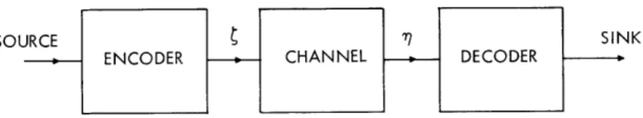
We intend to study some aspects of the problem of communication by means of a memoryless channel. A block diagram of a general communication system for such a channel is shown in Fig. 1. The source consists of M equiprobable words of length T seconds each. The channel is of the following type: Once each T/n seconds a real number is chosen at the transmitting point. This number is transmitted to the receiving
.th
point but is perturbed by noise, so that the 1 real number i is received as ri. Both
e and r are members of continuous sets and therefore the channel is time-discrete but amplitude- continuo us.
SOL IK
Fig. 1. Communication system for memoryless channels.
The channel is also memoryless in the sense that its statistics are given by a proba-bility density P(r1, 2' . i. ) so that
P(ril 2' ' i) = P ii (1)
where
P(rili )= P(rn1); i' = = i' (2)
and rli is independent of rj for i * j.
A code word, or signal, of length n for such a channel is a sequence of n real numbers (1, . . n). This may be thought of geometrically as a point in n-dimensional Euclidean space. The type of channel that we are studying is, of course, closely related to a bandlimited channel (W cycles per seconds wide). For such a bandlimited channel we have n = 2WT.
The encoder maps the M messages into a set of M code words (signals). The decoding system for such a code is a partitioning of the n-dimensional output space into M subsets corresponding to the messages from 1 to M.
For a given coding and decoding system there is a definite probability of error for receiving a message. This is given by
M
1 p (3)
e M =1 ei
where P is the probability, if message i is sent, that it will be decoded as a e.
message lother than i.
1
The rate of information per sample is given by
R = In M. (4)
n
We are interested in coding systems that, for a given rate R, minimize the probability of error, P
e
In 1959, C. E. Shannon studied coding and decoding systems for a time-discrete but amplitude-continuous channel with additive Gaussian noise, subject to the constraint that all code words were required to have exactly the same power. Upper and lower bounds were found for the probability of error when optimal codes and optimal decoding systems were used. The lower bound followed from sphere-packing arguments, and the upper bound was derived by using random coding arguments.
In random coding for such a Gaussian channel one considers the ensemble of codes obtained by placing M points randomly on a surface of a sphere of radius A; (where nP is the power of each one of M signals, and n = 2WT, with T the time length of each
signal, and W the bandwidth of the channel). More precisely, each point is placed independently of all other points with a probability measure proportional to surface area, or equivalently to solid angle. Shannon's upper and lower bounds for the probability of
error are very close together for signaling rates from some Rcrit up to channel capacity C.
R. M. Fano has recently studied the general discrete memoryless channel. The signals are not constrained to have exactly the same power. If random coding is used, the upper and lower bounds for the probability of error are very close together for all
rates R above some Rcrit.
The detection scheme that was used in both of these studies is an optimal one, that is, one that minimizes the probability of error for a given code. Such a scheme requires that the decoder compute an a posteriori probability measure, or a quantity equivalent to it, for each of, say, the M allowable code words.
In Fano's and Shannon's cases it can be shown that a lower bound on the probability of error has the form
P K e (R), (5a)
e
where K is a constant independent of n. Similarly, when optimum random coding is used, the probability of error is upper-bounded by
P >Ke -E(R)n E(R) = E (R) for R > R (5b)
P e
In general, construction of a random code involves the selection of messages with some probability density P(u) from the set U of all possible messages. When P(u) is such that E(R) is maximized for the given rate R, the random code is called optimum.
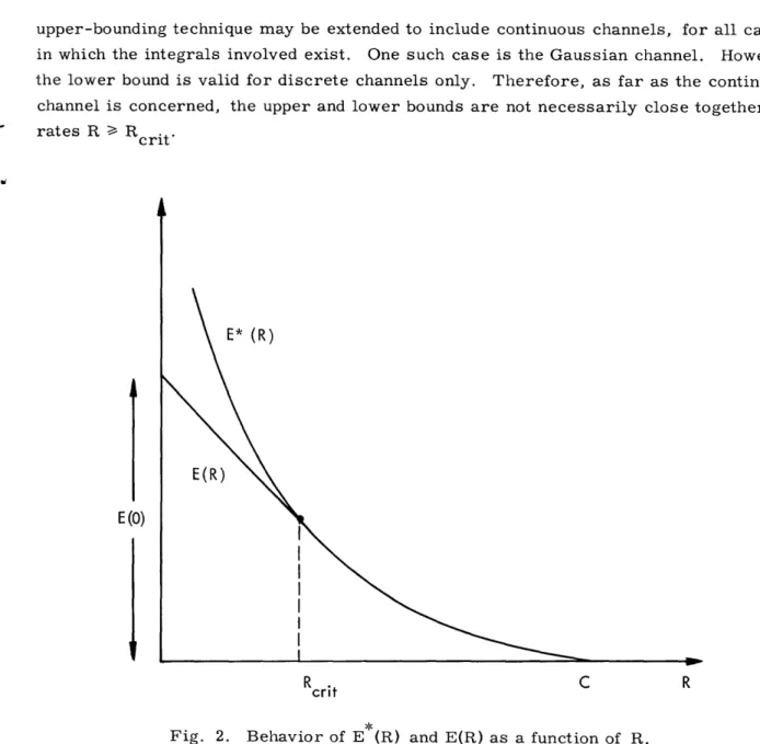
The behavior of E (R) and E(R) as a function of R is illustrated in Fig. 2. Fano's
2
upper-bounding technique may be extended to include continuous channels, for all cases in which the integrals involved exist. One such case is the Gaussian channel. However, the lower bound is valid for discrete channels only. Therefore, as far as the continuous channel is concerned, the upper and lower bounds are not necessarily close together for rates R > Rit
E (0)
E* (R)
Rcrit C R
crit
Fig. 2. Behavior of E*(R) and E(R) as a function of R.
The characteristics of many continuous physical channels, when quantized, are very close to the original ones if the quantization is fine enough. Thus, for such channels, we have E (R) = E(R) for R a Rcrit.
We see from Fig. 2 that the specification of an extremely small probability of error for a given rate R implies, in general, a significantly large value for the number of words M and for the number of decoding computations.
J. L. Kelly3 has derived a class of codes for continuous channels. These are block codes in which the (exponentially large) set of code words can be computed from a much smaller set of generators by a procedure analogous to group coding for discrete channels. Unfortunately, there seems to be no simple detection procedure for these codes. The receiver must generate each of the possible transmitted combinations and must then
3 _ ____II - -I I I I I I
compare them with the received signal.
The sequential coding scheme of J. M. Wozencraft, extended by B. Reiffen,5 is a code that is well suited to the purpose of reducing the number of coding and decoding computations. They have shown that, for a suitable sequential decoding scheme, the average number of decoding computations for channels that are symmetric at their out-put is bounded by an algebraic function of n for all rates below some R comp. (A channel with transition probability matrix P(yl x)is symmetric at its output if the set of proba-bilities P(Ylxl), P(yl x2), . . . is the same for all output symbols y.) Thus, the average
number of decoding computations is not an exponential function of n as is the case when an optimal detection scheme is used.
In this research, we consider the following aspects of the general problem of encoding and decoding for time-discrete memoryless channels: (a) Signal-space structure, (b) sequential decoding schemes, and (c) the effect of quantization at the receiver. Our results for each aspect are summarized below.
(a) Signal-space structure: A scheme for constructing a discrete signal space, in such a way as to make the application of sequential encoding-decoding possible for the general continuous memoryless channel, is described in Section II. In particular, whereas Shannon's workl considered code selection from an infinite ensemble, in this investigation the ensemble is a finite one. The engineering advantage is that each code word can be sequentially generated from a small set of basic waveforms. The effects of these signal-spare constraints on the average probability of error, for different signal power constraints, are also discussed in Section II.
(b) Sequential decoding schemes: In Section III we discuss the application of the sequential decoding scheme of Wozencraft and Reiffen to the continuous asymmetric channel. A lower bound on Rcomp for such a channel is derived. The Wozencraft-Reiffen scheme provides a bound on the average number of computations which is needed to discard all of the messages of the incorrect subset. No bound on the total number of decoding computations for asymmetric channels has heretofore been derived.
A new systematic decoding scheme for sequentially generated random codes is intro-duced in Section III. This decoding scheme, when averaged over the ensemble of code words, yields an average total number of computations that is upper-bounded by a
quantity proportional to n2, for all rates below some cutoff rate RComp
The corresponding probabilities of error of the two decoding schemes are also dis-cussed in Section III.
(c) Quantization at the receiver: The purpose of introducing quantization at the receiver is to curtail the utilization of analogue devices. Because of the large number of computing operations that are carried out at the receiver, and the large flow of infor-mation to and from the memory, analogue devices may turn out to be more complicated and expensive than digital devices. In Section IV, the process of quantization at the receiver and its effect on the probability of error and the receiver complexity are discussed.
II. SIGNAL-SPACE STRUCTURE
We shall introduce a structured signal space, and investigate the effect of the par-ticular structure on the probability of error.
2. 1 THE BASIC SIGNAL-SPACE STRUCTURE
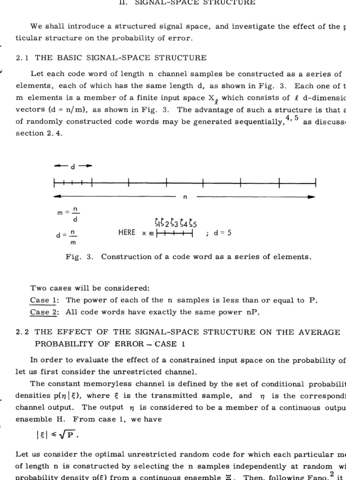
Let each code word of length n channel samples be constructed as a series of m elements, each of which has the same length d, as shown in Fig. 3. Each one of the m elements is a member of a finite input space X~ which consists of d-dimensional vectors (d = n/m), as shown in Fig. 3. The advantage of such a structure is that a set of randomly constructed code words may be generated sequentially,4' 5 as discussed in section 2. 4. - d
II
I
I
I
I
I
n nm
d d 2 3 ~4 5 d= n HEREx
=I--
I I-
; d= 5 mFig. 3. Construction of a code word as a series of elements.
Two cases will be considered:
Case 1: The power of each of the n samples is less than or equal to P. Case 2: All code words have exactly the same power nP.
2.2 THE EFFECT OF THE SIGNAL-SPACE STRUCTURE ON THE AVERAGE PROBABILITY OF ERROR - CASE 1
In order to evaluate the effect of a constrained input space on the probability of error, let us first consider the unrestricted channel.
The constant memoryless channel is defined by the set of conditional probability densities p(rl1 ), where ~ is the transmitted sample, and rl is the corresponding channel output. The output rl is considered to be a member of a continuous output ensemble H. From case l, we have
1
e1
V P.
(6a)
Let us consider the optimal unrestricted random code for which each particular message of length n is constructed by selecting the n samples independently at random with probability density p(S) from a continuous ensemble . Then, following Fano, it can
5
-be shown (Appendix A. 4) that the average probability of error over the ensemble of codes is bounded by
2e nE(R) R critrit < C P
e
L
e-nE(R)= e-n[E(0)-R] R R crit(6b)
where R = 1/n In M is the rate per sample, and E(R) is the optimum exponent in the sense that it is equal, for large n and for R a Rcrit' to the exponent of the lower bound to the average probability of error (Fig. 2). For any given rate R, p(g) is chosen so as to maximize E(R) [i. e., to minimize Pe].
Let us now constrain each code word to be of the form shown in Fig. 3, with the exception that we let the set X be replaced by a continuous ensemble with an infinite, rather than finite, number of members. We shall show that in this case, the exponent Ed(R) of the upper bound to the average probability of error for such an input space can be made equal to the optimum exponent E(R).
THEOREM 1: Let us introduce a random code that is constructed in the following way: Each code word of length n consists of m elements, where each element x is an d-dimensional vector
(7) selected independently at random with probability density p(x) from the d-dimensional input ensemble X. Let the output event y that corresponds to x be
(8) Here, y is a member of a d-dimensional output ensemble Y. The channel is defined by the set of conditional probabilities
d
P(YIX) =ATT P(il i) i=1 Also, let d p(x) = TT P(i) , i=l (9) (10)
where p({i) - p(~), for all i, is the one-dimensional probability density that yields the optimum exponent E(R). The average probability of error is then bounded by
>_ 2 exp[-nEd(R)] ; Rcrit -< R < C
e
exp[ -nE(R)] = exp[ -n[E d(0)-R] ]; R Rrit
(11)
where
6 X = 51, 2' -- " d
Ed(R) = E(R); Ed(0) E(0).
PROOF 1: The condition given by Eq. 10 is statistically equivalent to an independent, random selection of each one of the d samples of each element x. This corresponds to the construction of each code word by selecting each of the n samples independently at random with probability density p(~) from the continuous space I, and therefore by Eqs. 10 and 6, yields the optimum exponent E(R). Q. E. D. The random code given by (9) is therefore an optimal random code, and yields the opti-mal exponent E(R).
We now proceed to evaluate the effect of replacing the continuous input space x by the discrete d-dimensional input space x, which consists of vectors. Consider a random code, for which the m elements of each word are picked at random with proba-bility 1/1 from the set X of waveforms (vectors)
X = {Xk;k=l . ... . (13)
The length or dimensionality of each xk is d. Now let the set X be generated in the following fashion: Each vector xk is picked at random with probability density p(xk )
from the continuous ensemble X of all d-dimensional vectors matching the power con-straint of Statement 2-1. The probability density p(xk) is given by
p(xk) - p(x); k = 1, . (14)
where p(x) is given by Eq. 10. Thus, we let p(xk) be identical with the probability density that was used for the generation of the optimal unrestricted random code. We
can then state the following theorem.
THEOREM: Let the general memoryless channel be represented by the set of proba-bility densities p(ylx). Given a set X, let Ee, d(R) be the exponent of the average probability of error over the ensemble of random codes constructed as above. Let
E, d(R) be the expected value of E d(R) averaged over all possible sets Xa. Now define a tilted probability density for the product space XY
eSD(x Y)p(x) p(yIx) p(x) p(y x) 1-f(y)s
Q(x, y) = = (15)
f fX eSD(x Y)p(x) p(yI x) dxdy fy f p(x) p(y x)1-Sf(y)s dxdy
where [sp(x) p(y x)l-s dx 1 fly) = Q(y) p0 y s s -fy p(x) p(y I x) dy 7 __ __ 1_1_ (1 2)
p(x) p(y x)1 - s fx p(x) P(Y x)l-s dx 1 Part 1. E (R) > E(R) - In , d d exp[F1(R)] + - 1 (16) s and F1(R) are related parametrically to the rate R as shown below.
fY
[fX
p(x)
p(yx) 1 dx]dxdy
Q(y)2S-1 dy
1
R
fx f
Q(x,y)ln
Q(xl y)
p(x) dxdy >- Rcritx pYx
Rcrit= [R]s 2= Also, when R -< Rcrit
F 1(R) = F 1(Rcrit) = dE(O) = - ln p(x) p(y, x)1/2 dx dy; s= 12
2
Part 2. E, d(R) E( + ln d
exp[F2(R)] +
where F2(R) is related parametrically to the rate R by
0 F2(R) = ln
fX fY
p(x) y I 2(1-s) Q(y)2s-1 dxdy
f
[
P(x)P(ylx)l-s] Q(y)2s-1 dxdyR= 1 d xf Q(x y) 1 Q(x, y) ln p(x) dxdy - d ln exp[F2(R)d] + - 1 1 eE(0)d + _ 1 >A R -- In 11 eE(0)d + -Also, when R R crit -ndI
F 2(R)= F 2 (R ) = E(0) = - dln 2 2 crit d
fy [
p(x) p(y x)l/2 8 Then 0 < F 1(R) = n ; 0 s 2 (17) (18) (19) ; s 22 (20a) (20b) 12 dx dy. (21)Q(x I Y = QQ(xy) =
Q YY-
2
2 p(X) p(y X) 2 -s) Q(y) 2s-1 .. sPROOF: Given the set X, each of the successive elements of a code word is gener-ated by first picking the index k at random with probability 1/Q and then taking xk to be the element. Under these circumstances, by direct analogy with Appendix A, Eqs. A-46, A-41, and A-26 with the index k replacing the variable x, the average probability of error is bounded by
p(elX) exp[-nE(1)d(R)] + exp[-nE (R) (22)
where
E (1(R)= -R d d(tr) - rm (23)
E(2,d(R) = -d[Y ,d(S)-sDo] (24a)
TQ,d(t,r) = ln g ,d(t,r) (24b)
g d(t,r) = y kl p(k)p(k')p(yjk) exp[(r-t)D(ky)+tD(k', y)]dy; r 0; t O0
= 1 p(y1 i) exp[(r-t)D(xiy)+tD(x.y)] dy; with r 0; t 0, (24c)
fY i,1 - I
f(y)
D(ky) = D(xk,y) = n (25a)
P(YI xk)
Here, f(y) is a positive function of y satisfying fy f(y) dy = 1, and D is an arbitrary constant.
, d() = ln g d(S) (25b)
g,d() = jf k p(k) p(ylk) esD(ky) dy; 0 s
12 -p(yIxk) exp[sD(xky)] dy; 0 s (25c) As in Eq. A-47, let D be such that
EM'(R) = E 2 (R) (26)
Inserting Eqs. 23 and 24a into Eq. 26 yields
-R -d [, d(t,r) - r m-= -[ ,d(s) -s (27) -d ',d m Thus d m dQd(S) d id(tr) -R ] 1 (28) 9
_
I_
I__I_ _
I
Inserting Eq. 28 into Eqs. 23 and 24a yields E d(R) = E(1)d(R) = EQ )d(R)
s r r[ d(S) d d(r,t)
s -r d + s (29)
with 0 s, r 0; t 0. Inserting Eq. 29 into Eq. 22 yields p(elXI) 2 exp[-nE, d(R))] ,
where E d(R) is given by Eq. 29.,
We now proceed to evaluate a bound on the expected value of E , d(R) when averaged over all possible sets X. The average value of E , d(R), by Eq. 29, is
QEd(R) )s - r d, (s)+ s ,d( r, t)+sR]
with 0 < s, r _< 0, t _< 0. Inequality (30) is not an equality, parameters s, r, and t should be chosen so as to maximize input set X, rather than to be the same for all sets. From rithmic function, we have
(30) since, in general, the E
E d(R) of each individual the convexity of the
loga--ln x > -n x. (31)
Inserting Eq. 31 into Eqs. 24b and 25b yields
-TJ, d( s ) = -ln g, d(S) > -ln gQ, d(S) -y,t d( r t) > -n gp , d(r, t) .,
(32)
(33) Now, since r < 0, s > 0, we have
(34) r <0; s < 0
s -r s -r
Inserting (32), (33), and (34) into (30) yields
E (R) >-r s-rd 1 In g , d(S) s-rd - n g , d( ' s -r (35) From Eqs. 25c and 14, we have
g, d
8Y,
( ) =x
P(xk
k ) d( ) dxk=l
k 1fy fx
p(x) p(y I x) esD(xy) dxdy where the index k has been dropped, since p(xk) = p(x). Thusge d(S) =
f
f
p(x)p(ylx) eD(xy) dxdy. From Eq. 24c, we have10
q1
(36)
g r) = P( X d(t, ir)dxidxj (37) 1 b Here, by construction, = p(xi )p (x j ) ; i = p(x i) 6 (xi- j); p(xi xj) and, by Eq. 14, p(x) - p(x), (38) i=j for all i.
Thus, from (24c), (37), (38), and (39), we have g, d(r, t) = g, d(r, t) + g, d(r, t) , i j i=j where gQ, d(r, t) i*j 2 i.x 1 = P(xi)P(XJ)y P(YIXi) 1 j i~j
Q2 i=1 j Y X X p(x) p(x')
P(y
I x) exp[(r-t)D(x, y)+tD(x', y)] dxdx'dywith r 0; t 0, and
g, d(t, r)
i= j =2 i=1 Y X.1
P(Xi)
P(YI
xi) exp[rD(xi, y)] dxdy=2_1 il
fy
fX p(x)p(ylx) exp[rD(x,y)] dxdy; 2 i=1 Y Xr O
Inserting (25a) into (41) and (42) yields
y X ' Px p(x') P tp( x)l-r+t pyx')- tf(y)r dxdx'dyy g, d(r, t) = 2
i j
with r 0; t O;
:2 y fx
p(x) p(y Ix)l-r f(y)r dxdy with r 0.In general, f(y) of Eq. 25a should be chosen so as to maximize E , d(R) for each individual input set XF. However, we let f(y) be the same for all sets X and equal to the f(y) that maximizes the exponent Ed(R) for the unrestricted continuous set X. Thus
11 (39) (40) (41) (42) g, d(r, t) i=j (43) (44) _ _ __ __lil__
j
inserting Eqs. A-52 and A-53 into Eqs. 43 and 36 yields g d(r,t) = - exp[d(r, t)] Q 1 g d(r, t) = -exp[ d(r)] = gd(r) -i=j Thus, by Eq. 40, g,, d(r, t) = gd(r, t) + gd(r) Also, by Eqs. A-52 and 36,
g, d( s ) = gg, d( s )
Inserting Eqs. 47 and 48 into Eq. 35 yields
E 1d (R) > s - r r 1 In gd(s) d s s - r d ln[ R s - gd (rt) d s R r 1In s gd(r)/gd(r t) s-r d in gd(s) s 1r In gd(r t) 1 In[Ins Thus -rd s-rd -Thus (47) (48) + - 1 sS R. E d(R) s - r d sr s-rd d(S) d -rd d(r,t) srdln , t)] + -(49) Now, the exponent Ed(R) that corresponds to the unconstrained d-dimensional con-tinuous space X is given by Eq. A-49:
Ed(R) Eliminating = D y lds - S -m Eliminating Do yields
Ed(R) =r 1 s d 1 (r t) r R.
d( - r d d s - r d s-rr (50)
Furthermore, Ed(R) is maximized, as shown in Eqs. A-50, A-51, A-54, A-55 and A-56, by letting
p(x) (y x)1- dx f(y) =
f
[f
p(x) p(yj x)
1dxl
dy
r = 2s - 1; t = s -1 For R Rcrit s is such that
(51a) (51b) 12 gd(r, t) (45) (46) ---R + d d (r(7t) m
R [(s-l)H7d,()- d(s)]; 0 < s 22'
2 ' (51c)
where
Rcrit= [R]s=1/2.
If we let the parameters r, s, and t of (49) be equal to those of (50), we have
E d(R) >- Ed(R) 1, d d s s - r d In exp[yd(r)-d(r, t)] +
The insertion of Eq. 51b yields
s 1 ( R ) ] +exp[F1+ E, d(R) > Ed(R) 1 s d . -1] where
F1(R) = d(2s-1) - 7d(2s-l;s-1).
Inserting Eqs. A-52 and A-53 into Eq. 54 yields
F1 (R) = In
ffx
p(x) p(y x) 2-2s[ f(y)]2s-1 dxdy-In
fy fx
f p(x)p(x')p(ylx)lisYX X p(ylx)l-s f(y)2s-1 dxdx'dy.
fx P(X)p(ylx)2(1-s)f(y)2 l-1 dxdy F1(R) = In
p(x)p(yx)l-s dx] K
(55) f(y)2s-1 dxdy
where s and F1(R) are related parametrically to the rate R by Eq. A-60c, for all rates above Rcrit = [R]s=1/2
As for rates below R crit we let
1 1
s= ; 2' t= -; 2' r = 0. (56)
Inserting Eq. 56 into Eqs. 54 and 55, with the help of Eqs. A-69 and A-71, yields
[F(R)]s=1/2 = -ln fy [fx p(x)p(yjx) /2d = dEd(O) (57) where Ed(O) = [Ed(R)]R=O 13 -11
i
(52) (53) (54) Thus P . " II~~~~~~~~~~~~~~~-~ ~~ ~ ~~~~~~~~~~~~~I~~~
- , IR exp 1(R) s=12]+ - 1 E d(R) >, E(R) In = E(R) -ln (exp[dEd(0)] + - 1) d
for R < Rcrit From Eqs. 14 and 12 we also have Ed(R) E(R) for all rates, by con-struction. The proof of the first part of the theorem has therefore been completed (a simplified proof for the region R < Rcrit is given elsewhere ). Q. E. D.
In order to prove the second part, let us rewrite (49) as
E d(R) ) d( s _
[R
+ 1ln Qs - ( r d s -rd 't )t s s [R] r 1here s 1 [R], where R' = R + ln d exp[yd(r)- yd(r, t)+ - 1 Q (58) exp[yd(r)- yd(r, t)] + - 1 (59) Comparing (59) with (50) yieldsE, d(R) > Ed(R') =EdR + 1In exp[F2(R)] + - 1 By Eqs. 51a, 55, A-57, A-58, A-59, A-60c, and A-60b, cally to the rate R by
F2(R) = in
R' = R + In d
f
fx P(x)p(yx) 2(1-s)Q(y)2s -1 dxdyfy [
p(x)p(ylx) dxj Q(y) 2s-1 dxdyexp[F2(R)] + - 1 Q(x1y)
-
d fxf
Q(x,y) ln p(x) ; (60) F2(R) is related parametri-(61) 2 0 < S 2 2 (62) for all R' > R' = [R']s= crit s=1/2 Inequality (63) can be rewrittenexp[F2(R) ]+ - 1 1 R >- Rcrit -In = n dE(O) + _ 1 = Rcrit d 14 t (63) (64) -·
1 In As for rates below R -In
crit d
edE(O) + - 1
e , we let
1 1
s = t = -2 r= O.
Inserting (65) into (60) and (61) yields
E d(R) > E
~,
d dd + d In eIcrit+_
R R(65)
(66) From Eqs. 14 and 12, by construction, Ed(R) E(R) for all rates. Thus, the proof of the second part of the theorem has been completed.
Q.
E. D. Discussion: We proceed now to discuss the bounds that were derived in the theorem above. We shall consider particularly the region 0 -< R -< Rcrit' which, as we shall see in Section III, is of special interest. From Eqs. 16 and 18,E (R) > E(R) - 1 n[edE(+ 1]
, d d I for R < Rit.crit '
From Eq. 6, we have
for R -- Ritcrit ' Inserting (68) into (66) yields
[dE() +
-E, d(R) > E(0) - R -d n -Now, whenever dE(O) << 1, we have
1 ldE(O)+ E d(R) E(O) - R T In E(O) - R - In 1+ ) d 1 -E(O) - R - E(0) E a, d d(R) E(O) I -,el1 -R, Thus for R -< Rcrit. for R -< Rcrit.
for R - Rcrit' and dE(O) << 1.
Comparing (71) with (68), we see that El, d(0) can be made practically equal to E(R) by using quite a small number , of input symbols, whenever E(O)d << 1. In cases in which
-max
d
0 and dp(r 0 so that p(rj I) can be replaced by the first two terms I elmax d~ d=0dp(r 1
I
)of the Taylor series expansion, p( 1) |p(=M I0) + d= , it can be shown (by insertion into Eqs. A-74a-d) that the optimum input space consists of two oppositely directed vectors, mamax x and - mamax'x' for all rates 0 < R < C, and that
15 E(R) = E(O) - R (67) (68) (69) (70) (71)
_____ ._
I
0.1 1 2
[=
E(0) =C = 4max do
P(,71 o)
where C is the channel capacity. Inequality (69) may be bounded by
E(O)d
Qd d + f crit
= E(O) - R - d-ln [eE(O)d + 1] (72)
Thus, whenever dE(O) >> 1, we have from (72)
El d(R)E(. EE d(R) 1 dn In [e E(O)d - In [ - In - R (73) when In << E(O) d and E ,d(R) E() R - n [ E ( ) d - l n +1] 1 -[In e-E(O)d]R (74) E(0) (74) when In >> E(O) d
Comparing Eqs. 73 with 74 yields
E(R) > E, d(R) - E(R); R - Rrit dE(O) >> 1 (75) or
E, d(R) E(R) (76)
if
-In Q > E(O) dE(O) >> 1. (77)
d
In the following section we shall discuss the construction of a semioptimum finite input set X for the Gaussian channel. [A semioptimum input space is one that yields
an exponent E, d(R) which is practically equal to E(R).] We shall show that the number of input vectors needed is approximately the same as that indicated by Eqs. 75 and 71. This demonstrates the effectiveness of the bounds derived in this section.
2.3 SEMIOPTIMUM INPUT SPACES FOR THE WHITE GAUSSIAN CHANNEL -CASE 1
The white Gaussian channel is defined by the transition probability density
16
p(r |) = _ exp ( (78)
vf r 2 2 in which, by inequality (6a),
l1
-l< I Imax \-P (79)Let us define the voltage signal-to-noise ratio A, as
A=-. (80)
Inserting (79) into (80) yields
A A Amax (81)
max a ar
We shall first discuss the case in which
dAmax << 1 (82)
max
and proceed with the proof of the following theorem.
THEOREM: Consider a white Gaussian channel whose statistics are given by Eq. 78. Let the input signal power be constrained by (79) and by (82). Let the input space con-sist of two d-dimensional oppositely directed vectors. Then the exponent of the upper bound to the probability of error, E2 d(R) is asymptotically equal to the optimum exponent E(R).
PROOF: From Eq. 7 we have x = 1' 2 . . .I d'
The input set X2 consists of two oppositely directed vectors. Let those two vectors be
xl = ' f .... d (83)
1 2 d'
1 1 1
where 1 = 2= 21 = d max' andand
2= 2 2 (84)
2 2 2
where t1 = ~2= *-- 1 2 = d - maxmax' From Eqs. 8 and 9 we have
Y = r1 72 .2' rid and d p(yxI ) = rT P((i i) -i=l 17 ___
I
_
__
Inserting Eqs. 78, 83, and 84 into Eq. 9 yields d p(yIx1) = I i=l d P(Yl X2) = i=l 1 exp( (2 )d/2 Td 1 (2 T)d/2 Td i ( i-max)2 20r2 (7 i + max) 2 exp 2 2- /
From Eqs. 29 and 30 we have p(e X2) 2 exp[-nE2, d(R)] where (R) r 1 s r 1 2, d s - r d 2, d s - r d 2, Let r = 2t + 1; s=l+t; 0 <s - 12 2 and let d f(y) = p(y[ O) = 1 i=i (27r)d/2 d
(
2\ exp ri 20 and 1 p(x1) = P(X2) = 2Inserting Eqs. 88, 89, and 90 into Eqs. 24b, 25, and 87 yields E (R) = 1 - 2s 1 s 1 (2-1, s-) s R
2, 1 -s d2,d 1 2, - - 1-ss
l p(y xi)l1-s p(yI O)S dy
1-s l-s 2s-1
Y2, d( 2s-l,s-1) = n i4 p(yx ) p(yxj Inserting Eqs. 85 and 89 into Eqs. 92 and 93 yields
1 , d(S) = In -
1f
F
rl 1 -i J_ 1exp 712 tr = ln2
2 exp -exp(
(1 -s)(- max)max) + (1-s)(r+ max)2 + 2 2 2 max(1- s) sd 2o-2 2 2Ž d4 ]} rl - d rl 2 -ds(1-s)<1 -- max 2o -' - 2 18 (85a) (85b) I (86) t) -s s S- r R. (87) (88) (89) (90) 2 Y2, d( s ) = n1
y (91) (92) (93)I
d
dr17 (94) ----\
5'2, d(2s-1, s-1) 1zr/ 1 / 2(1-s)(r1- )2 + (2s-1) rl2 = In f exp - 2max2
/
4 77 a- I~r2-7r 2cr 1 ,\( r ' exp - 2(1-s)(+ max) 2 + (2s-1) max 2 2 2¢r/
d d Y] d] (1-s)( -max ) 2 - ( 1-s +)(7 + max) - ( 2 s -1 ) rl 2 2 2(r2 2 1SF
+2 f2 = In {2 exp 4 maxd[2(1-s)-4(1-s)2] ) 222 d} d ]} 2(1-s)2 dl + 2 exp max 22 j i 2Now, since by (82) dA2max
2 max a<< 1, we have 2 a' 2 (95) 2 d(2S-1, s-1) in 1 2 - max d[2(1-s)-r(I-s) 21 2 2 2 maxd 2(1-s) 2 2 = n 1 max 2ds(l-s) 2m 2
2
max 2ds(l-s)= 2 (s) 2 Inserting 2, 91 yields Inserting Eqs. 94 and 96 into Eq. 91 yieldsE2, d(R)= +[ L-ss(-s)-s 2 max s R 2ff2 1 - s 2 2 1-s A2 max S
1
=s 2 1 s R; 0 s < Maximizing E2 d(R) with respect to s yields1 1 A2
for R crit 8 max
2 crt8 max
s = 1 for R Rrit crit = 8 Amaxmax
19 (96) (97) _____ _
_II
?2 I exp i 7 a(
Thus
E ( R ) 1 A2 -R -R; R 1A2A
(98a)
2, 4 d max 8 max
E2, d(R) - 2 A +R; 8 max 2 max (98b)
Comparing Eqs. 98 with the results given by Shannon yields
E(R) -- E2 d(R) - E(R) (99)
Shannon's results1
are derived for the power constraint of Case 2, and are valid also in cases where the average power is constrained to be equal to P. The set of signals satisfying Case 1 is included in the set of signals satisfying the average power constraint above. Thus, Shannon's exponent of the upper bound to the probability of error is larger than or equal to the optimum exponent E(R) which corresponds to the constraint of Case 1. Thus, from (99),
E2 d(R) E(R) (100)
for A2 d << 1 . Q.E.D.
We shall now discuss cases in which the condition of (82) is no longer valid. The first step will be the evaluation of E , d(0) for the white Gaussian channel. From Eqs. A-69 and A-71 we have
E~ d(0) = d n L E P(x)P(x')
fy
p(ylx) /2 p(y x')1/2 dy. (101)Inserting Eqs. 9 and 78 into (101) yields
E (0) = n p(x) p(x')
r
,
ex[ - d (102)where x t1 f2) d and x ' d 2', 1 .. , 5 Thus 2 1 EEd(0) =- In (x)p(x)
f
1 exp [ d d ln v' v' L Yp(x)p(x) exp L 2 (103) _XI_11_ XX' 8 cLet D be the geometrical distance between the two vectors x and x', given by
2 = [x-x' = - -d )p (104)
Then, inserting (104) into (103) yields
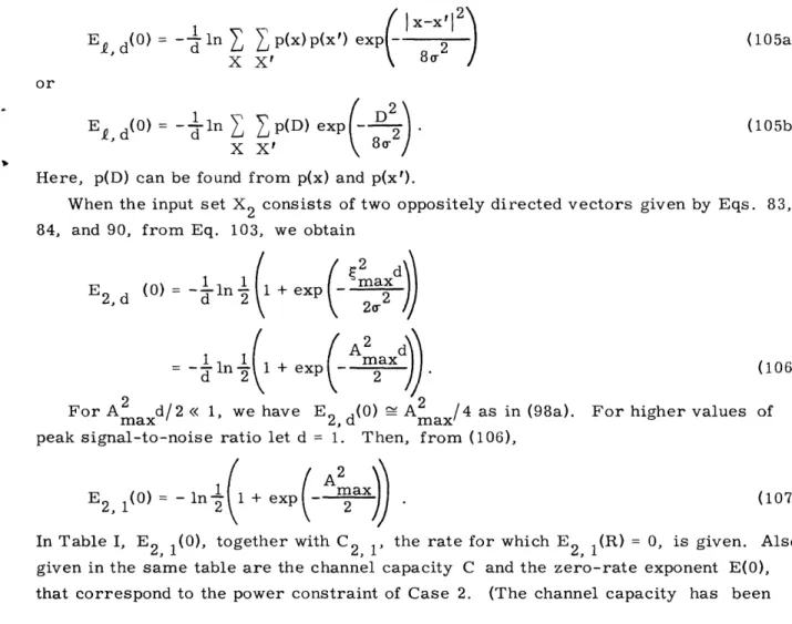
(105a) E, d(0) = - In p(x)p(x') exp- c 2
Q. d X X'
(
2)(105b)
Here, p(D) can be found from p(x) and p(x').
When the input set X2 consists of two oppositely directed vectors given by Eqs. 83, 84, and 90, from Eq. 103, we obtain
(2 d
+ exp 21
2cr2
= -1 in 1 + exp(A max d
For Aaxd/2 << 1, we have E d(0) Aax/4 as in (98a). For higher values peak signal-to-noise ratio let d = 1. Then, from (106),
(106) of
E2, 1(0) =in 2 ( + exp Aax
In Table I, E2 1(0), together with C2, 1 the rate for which E2, 1(R) = 0, is given. Also given in the same table are the channel capacity C and the zero-rate exponent E(0), that correspond to the power constraint of Case 2. (The channel capacity has been
Table 1. Tabulation of E2 1(0) and C2 1
2, 1 a 2, 1 vs Amax 21 or E2,d (0) = -dn (107) Ab 1B~ 1(0) 2(O) C
C
C 2 1CK
max
22, 10)
2 (0)C
1(O) 2, 1 1 0.216 0.22 0.99 0.343 0.346 0.99 2 0.571 0.63 0.905 0.62 0.804 0.77 3 0.683 0.95 0.72 0.69 1.151 0.60 4 0.69 1.20 0.57 0.69 1.4 0.43 --- I---" "---computed by F. J. Bloom et al.,9 and E(O) is given by Fano2 and is also computed in Appendix B.) The channel capacity C and the zero-rate exponent E(O) for Case 1 are
upper bounded by the C and E(O) that correspond to the power constraint of Case 2. From Table I we see that the replacing of the continuous input set by the discrete input
set X2, consisting of two oppositely directed vectors, has a negligible effect on the exponent of the probability of error because Amax2 1.
X1
- MAX
x6
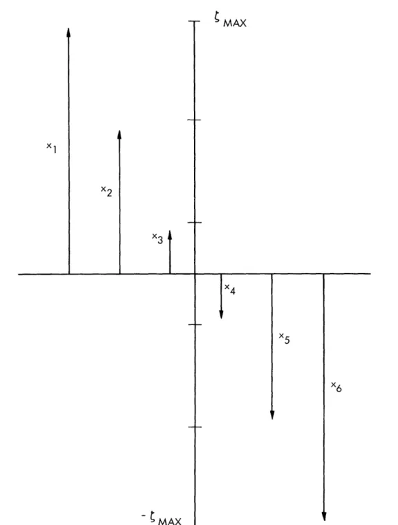
Fig. 4. Semioptimum input space for the Gaussian channel.
22
Let us consider, next, the case in which the input set X$ consists of one-dimensional vectors as shown in Fig. 4.
vectors is
2 max D min = - 1 Let
p(x) 1 = I ;
The distance between each two adjacent
(108)
i= 1,.... . (109)
Inserting (108) and (109) into (105) yields
E2 1(0) -ln [+ 2 ( Q-k)
k=1
m(kDin exp - 8r 2
8 a-Thus, since 4k < k2; k > 2, we have
E2 1() >- -ln + 2(-1) exp -in
I
2 + 2(f-1) exp(-
n
41
Now define K as A - 1 =max K '+[
min + k - 2 Q 4kD . 2(f-2) ~ exp - 2 i k=1 82 8r 2 D.inmn - 2(Q-2) 8rU2 ) 2 exp min + 28 2
exp( 4kD n/ 8a2) exp( 4Dm2/8o2) 1 1 exp 4D min. /8 ) 1i} 0 K.Inserting (112) and (81) into (108) yields D = 2arK.
min
Inserting (113) into (111) then yields
E2, 1(0) > In (1+KAmax) - n {1 + 2 exp -- 2 ) +22
If we choose l so that K 1, we have E2, 1(0) = n (+Amax ) - In 2, 52.
From Eqs. 114b and 112, for A max >> 1, we have
23 (110)
I
(111) (112) (113) (114a) (114b) --- I^" ,~ -_ - - R_E2, 1(0) In Amax (115a)
In In Amax = E2, 1(0). (115b)
On the other hand, it can be shown (Appendix B) that
E(0) In Amax; Amax >> 1 . (116)
Thus, by (116) and (115), we have
E2, (R) E(R); R < Rcrit Amax >> 1 (117a)
For
In = E(0); d = 1. (117b)
Comparing Eqs. 71 and 75-77 with Eqs. 100 and 117, respectively, gives the result that the lower bound on EQ d(R) previously derived is indeed a useful one.
2.4 THE EFFECT OF THE SIGNAL-SPACE STRUCTURE ON THE AVERAGE PROBABILITY OF ERROR- CASE 2
For a power constraint such as that of Case 2, we consider the ensemble of codes obtained by placing M points on the surface of a sphere of radius n-P.
The requirement of Case 2 can be met by making each of the m elements in our signal space have the same power dP (see Fig. 3). (The power of each word is mdP= nP and therefore Case 2 is satisfied.) This additional constraint produces an additional reduction in the value of E, d(R) as compared with E(R). Even if we let the d-dimensional input space Xf be an infinite set ( = o), the corresponding exponent Ed(R), in general, will be
Ed(R) - E(R). (118)
The discussion in this section will be limited to the white Gaussian channel and to rates below Rcrit Thus
Ed(R)= Ed(0) -R; R -< Rcrit. (119)
Let
Ed(0) = E(0) - kd(A2) E(0), (1 20a)
where
A2 P
A - P (120b)
Then, from (119) and (120), we have
Ed(R) = E(0) - kd(A 2) E(0) - R; d d R -< Rcrit. crit~~~~~~~~~~~~~~~~(11 (121)
24
We shall now proceed to evaluate kd(A2) as a function of A2 for different values of d.
The input space X is, by construction, a dimensional sphere of radius dP.
I-/11
set of points on the surface of a
d- N-/
I
\0
/
I
I
NFig. 5. Cap cut out by a cone on the unit sphere.
Let each point of the set X be placed at random and independently of all others with probability measure proportional to surface area or, equivalently, to solid angle. The probability Pr(O0-<o01) that an angle between two vectors of the space X is less than or equal to o01 is therefore proportional to the solid angle of a cone in d-dimensions with half-angle 01. This is obtained by summing the contributions that are due to ring-shaped elements of area (spherical surfaces in d-l dimensions of radius sin 0 and incremental width dO as shown in Fig. 5). Thus the solid angle of the cone, as given by Shannon,1 is
) 7r(d-)/ 2 1
0 (sin 8) do. (122)
Here we have used the formula for the surface sd(r) of a sphere of radius r in d-dimensions, sd(r) = d/2 rd-1 / r(d/2+1). From (122), we have 25 - --c-- -1"11 - - II- . .-e1 ( 1 )
=
Pr(O-<0 1) Q2(7) 0(- (-)/ 1
r d )
d1 ( d+2) 01 ( 0 1(
+ )
0 11 7r
JO
d d/ 2Ir(
)
(sin 0) dO sin ) do.The probability density p(O) is therefore given by
d(Od 0-< 0 1) 1 (2)
p(o) = do
I VTr
(sin 0)d - 2 (124)
Now, by (104), the geometrical distance between two vectors with an angle between them (see Fig. 5) is
D = 4(dP sin2-) .
Inserting (125) and (124) into (105b) yields
(125)
7r
Ed(O) = -1n
(
2dP.2
p(O) exp -- sin2 do
2o2 2
1 {n 1 () dln ' F d_ ) f
exp -dP sin2
22 (sin 0)d-2 d0
ting (120b) into (126) for d 2 yields
1 Ed(O) = - in f expI 1 Tr 0~.·
r()
V r %d-l)V-2-)
dA
2 2 exp dA)f
7T 0sin2 (sin o)d-2 de
xdA2
exp 4 cos 0 sin Od- 2 dO
Equation 127 is valid for all d > 2. As for d = 1, it is clear that in order to satisfy the power constraint of Case 2 the input space X must consist of two oppositely directed
26 Is (123) Insert or (126) Ed(O) Ed(0) = - -ln (127a) (127b)
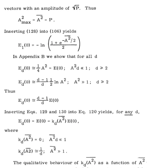
vectors with an amplitude of Th.
2 2=P.
A = A = . max
Inserting (128) into (106) yields
E1(0) = - in + eA2
In Appendix B we show that for all d 1 2 Ed(0) - A = E(0); Ed(0 ) _d d - 11n A2 ; - d 2 A2d<< 1; d 2 A2 >> 1; d 2 Thus Ed(0) d - 1E(0)
Inserting Eqs. 129 and 130 into Eq. 120 yields, for any d, Ed(0) = E(O) - kd(A2)E(0),
where
_ 2
kd(A2) = 0; A2d << 1 kd(A2) ; A2 >> 1.
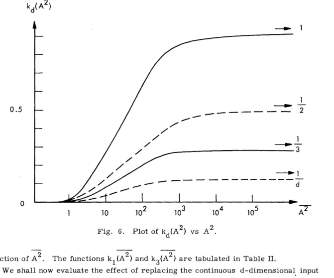
The qualitative behaviour of kd(A2) as a function of A2 with d as a parameter is illustrated in Fig. 6. From (127a) it is clear that Ed(0) is a monotonic increasing
Table 2. Tabulation of k1(A2) and k3(A2) vs A2.
27 (128) (129) (130a) (130b) (130c) (131) A2 k (A2 ) k3(A 2 ) 1 0.01 4 0.095 0.046 9 0.28 0.095
16
0.43
0.135
100
0.7
0.2
104
0.9
0.28
-
l
- -Thusk (A2)
0.5
n
1 10 103 10 10 5
Fig. 6. Plot of kd(A2) vs A2 .
function of A2. The functions kl(A2 ) and k3(A2) are tabulated in Table II.
We shall now evaluate the effect of replacing the continuous d-dimensional input space X by a discrete d-dimensional input space X,, which consists of vectors.
Let each of the m elements be picked at random with probability 1/Q from the set X of vectors (waveforms), X - {xk:k=l, .. }.,
Let the set X be generated in the following fashion: Each vector xk is picked at random with probability p(xk) from the ensemble X of all d-dimensional vectors matching the power constraint of Case 2. The probability p(xk) is given by
p(xk) (x)x=x; k = 1 ...
where p(xk) is the same probability distribution that is used to generate Ed(0). The following theorem can then be stated.
THEOREM 2: Let E, d(0) be the zero-rate exponent of the average probability of error for random codes constructed as those above. Let E , d(0) be the expected value of EQ, d(0) averaged over all possible sets X . Then
1 e x p [ d E d ( 0 ) ] + - 1
ES, d(0 Ed(O) d + - . (132)
The proof is identical with that of Theorem 1. Inserting (131) into (132) yields
1 exp[dEd( 0 )] + - 1 )
E d(0) > E(0) - kd(A 2)E(0) - exd + - (133)
Thus there is a combined loss that is due to two independent constraints:
1. Constraining the power of each of the input vectors to be equal to dP; the resulting loss is equal to k (A2) E(0).
2. Constraining the input space to consist of vectors only; the resulting loss is 1 exp[dEd(0)I + - 1
equal to Iln e
We now evaluate the effect of these constraints at high (and low) values of A . From
(132) we have
1 (exp dEd(0)]+ A E d(O) Ed() Ed(0) de n - +
= Ed(0) - in exp(dEd(0)-ln)+l ) . (134)
Thus, for E(0) - In A2 >> 1, we have
() d n << Ed(0) _ d - n 2 (135a)
E- d(°0 Ed(0); d In Q >> Ed(o) d 1 n A2 (135b) On the other hand we always have E d(0) -< Ed(O), and inserting it into (135b) yields
E d(0) - Ed(0) = d - 1 1 n A2 (136)
fi, d d d 2
for d n >> Ed(0).
Whenever A2d << 1, an input space X2 that consists of two oppositely directed vectors with an amplitude of
VdP
yields the optimum exponent E(R) for all rates 0 < R < C, as shown in section 2. 3.2.5 CONVOLUTIONAL ENCODING
We have established a discrete signal space generated from a d-dimensional input space which consists of input symbols. We have shown that a proper selection of and d yields an exponent E , d(R) which is arbitrarily close to the optimum exponent E(R).
We proceed to describe an encoding scheme for mapping output sequences from an independent letter source into sequences of channel input symbols that are all members of the input set X . We do this encoding in a sequential manner so that sequential or other systematic decoding may be attempted at the receiver. By sequential encoding we mean that the channel symbol to be transmitted at any time is uniquely determined
29
by the sequence of the output letters from the message source up to that time. Decoding schemes for sequential codes will be discussed in Section III.
Let us consider a randomly selected code with a constraint length n, for which the size of M(w), the set of allowable messages at the length w input symbols, is an expo-nential function of the variable w.
M(w) AeWRd; 1 < w < m, (137)
1
where A is some small constant 1.
A code structure that is consistent with Eq. 137 is a tree, as shown in Fig. 7. There is one branch point for each information digit. Each information digit consists of "a" channel input symbols. All the input symbols are randomly selected from a d-dimensional input space X~ which consists of vectors. From each branch point there diverge b branches. The constraint length is n samples and thus equal to m input symbols or i information digits where i = m/a.
The upper bound on the probability of error that was used in the previous sections and which is discussed in Appendix A, is based on random block codes, not on tree codes, to which we wish to apply them. The important feature of random block codes, as far as the average probability of error is concerned, is the fact that the M code words are statistically independent of each other, and that there is a choice of input symbol a priori probabilities which maximize the exponent in the upper bound expression.
In the case of a tree structure we shall seek in decoding to make a decision only about the first information digit. This digit divides the entire tree set M into two sub-sets: M' is the subset of all messages which start with the same digit as that of the transmitted message, and M"' is the subset of messages other than those of M'. It is clear that the messages in the set M' cannot be made to be statistically independent. However, each member of the incorrect subset M"' can be made to be statistically independent of the transmitted sequence which is a member of M'.
Reiffen5 has described a way of generating such randomly selected tree codes when the messages of the incorrect subset M" are statistically independent of the messages in the correct subset M'.
Thus, the probability of incorrect detection of the first information digit in a tree code is bounded by the same expressions as the probability of incorrect detection of a message encoded by a random block code.
Furthermore, these trees can be made infinite so that the above-mentioned sta-tistical characteristics are common to all information digits, which are supposed to be emitted from the information source in a continuous stream and at a constant rate. These codes can be generated by a shift register,5 and the encoding complexity per information digit is proportional to m, where m = n/d is the number of channel input symbols per constraint length.
Clearly, the encoding complexity is also a monotonically increasing function of (the number of symbols in the input space X). Thus, let Me be an encoding complexity
measure, defined as
M= m = n- (138)
e d
The decoding complexity for the two decoding schemes that will be discussed in Section III is shown to be proportional to me, 1 a - 2, for all rates below some computational cutoff rate R
comp
Clearly, the decoding complexity must be a monotonically increasing function of . Thus, let Md be the decoding complexity measure defined as
d
MdYE Cm2= n - (139)
We shall discuss the problem of minimizing Me and Md with respect to and d,
for a given rate R, a given constraint length n, and a suitably defined loss in the value of the exponent of the probability of error.
2.6 OPTIMIZATION OF AND d
This discussion will be limited to rates below R rit, and to cases for which the power constraint of Case 1 is valid. Let L be a loss factor, defined as
E(0) - El d(0)
L = ' (140)
E(0)
Now, for rates below Rcrit' from Eq. A-70, we have E , d(R)= E , d(0) -R; R -< Rcrit.
Thus
E, d(R) E(0)(1-L) - R; R Rcrit (141)
Therefore specifying an acceptable E , d(R) for any rate R Rcrit, is equivalent to the specification of a proper loss factor L.
We proceed to discuss the minimization of Me and Md with respect to Q and d, for a given acceptable loss factor L, and a given constraint length n.
For dE(O) << 1, from Eq. 71, we have
E( d> a( 1 - ; dE(0)<< 1, R Rcrit. (142)
Inserting (140) into (142) yields
Tu ; E(0)d << 1; R Rcrit
Thus, by Eqs. 138 and 139, we have
31
M L n E(O)d << 1 (143a) e Ld'
2
Md n 2; E(O)d<< 1 (143b)
Ld
The lower bounds to Me and Md decrease when d increases.
Thus, d should be chosen as large as possible and the value of d that minimizes Me and Md is therefore outside the region of d for which E(O)d << 1. The choice of Q should be such as to yield the desired loss factor L. Also, by Eq. 72,
E d(0) > E(0) ln ( E(O)d + R R Rcrit (144)
This bound is effective whenever Q >> 1. This corresponds to the region E(O)d >> 1. (In order to get a reasonably small L, should be much larger than unity if E(O)d >> 1.) Inserting (144) into (140) yields
L = d1 n E()d + 1). dE(O) Thus eE(O)d = e (145) eLE(O)d
Inserting (145) into (138) and (139) yields E(O)d Me <n eE(O)d (146a) eLE()d 2 E(O)d Md <n2 e (146b) d d2 LE(O)d e -l
From (146a), the bound to Me has an extremum point at
E(O)d - 1 eE()d (147)
E(0)d(l-L) - 1
if a solution exists. Thus, for E(O)d >> 1, 1 eLE(O)d
1-L or
dE(0) = L ln l-L'1
Now, for reasonably small variables of the loss factor L, we have
dE(O) 1. (148)
32
This point is outside the region of d for which dE(O) >> 1. From (146b), the bound to Md has an extremum point at
E(O)d - 2 LE(O)d E(O)d(l-L) - 2
if a solution exists. Thus, for E(O)d >> 1,
1 LE(O)d
1 -L or
dE(O) In 1 L
For reasonably small variables of the loss factor L, therefore, we have dE(O) 1. This point is outside the region of d for which dE(O) >> 1.
We may conclude that the lower bounds to Me and Md are monotonically decreasing
functions of d in the region dE(O) << 1, and are monotonically increasing functions of d in the region dE(O) >> 1.
Both Me and Md are therefore minimized if
E(O)d 1; E(0) 1, R < Rcrit (150a)
And since d > 1, if
d = 1; E(0) 1, R -< Rcrit crithe desired loss factor L. (150b) The number is chosen to yield the desired loss factor L.
33
__ _
III. DECODING SCHEMES FOR CONVOLUTIONAL CODES
3. 1 INTRODUCTION
Sequential decoding implies that we decode one information digit at a time. The symbol si is to be decoded immediately after si-1 Thus the receiver has the decoded set (... ., s1 so) when it is about to decode s . We assume that these symbols have been decoded without an error. This assumption, although crucial to the decoding pro-cedure, is not as restrictive as it may appear.
We shall restrict our attention to those st that are consistent with the previously decoded symbols.
3.2 SEQUENTIAL DECODING (AFTER WOZENCRAFT AND REIFFEN)
Let u be the sequence that consists of the first w input symbols of the transmitted sequence that diverges from the last information digit to be detected. Let u be a
w
member of the incorrect set M". Therefore u' starts with an information digit otherw than that of the sequence uw. Let vw be the sequence that consists of the w output symbols that correspond to the transmitted segment uw. Let
p(vw)
D (u,v) = In (151)
P(Vw luw)
We call this the distance between u and v, where
w
p(vw) =T7 P(Yi)
w
P(vwluw) = [7 P(yi xi)
Let us define a constant Dj given by
W
P D(UV) < e J (152a)
where k. is some arbitrary positive constant that we call "probability criterion" and is J
a member of an ordered set
K = {k:k.=k. + k. =E(R)n , (152b)
max where A O0 is a constant.
Let us now consider the sequential decoding scheme in accordance with the following rules:
1. The decoding computer starts out to generate sequentially the entire tree set M (section 2. 5). As the computer proceeds, it discards any sequence
u'
oflnt1 1 w length w symbols (1 w m) for which the distance D(u',v) > D . (D is for
the smallest "probability criterion" kl).
2. As soon as the computer discovers any sequence M that is retained through length m, it prints out the corresponding first information digit.
3. If the complete set M is discarded, the computer adopts the next larger cri-terion k2, and its corresponding distance D; ' (1 - w m).
4. The computer continues this procedure until some sequence in M is retained through length m. It then prints the corresponding first information digit.
When these rules are adopted, the decoder never uses a criterion K. unless the J
correct subset M' (and hence the correct sequence uw ) is discarded for kj_1 The
probability that uw is discarded depends on the channel noise only. By averaging both
over all noise sequences and over the ensemble of all tree codes, we can bound the required average number of computations, N, to eliminate the incorrect subset M". 3.3 DETERMINATION OF A LOWER BOUND TO RCOMP OF THE
WOZENCRAFT-REIFFEN5, 6 DECODING SCHEME
Let N(w) be the number of computations required to extend the search from w to w + 1. Using bars to denote averages, we have
N=
N(w).
w
N(w) may be upper-bounded in the following way: The number of incorrect messages of length w, M(w), is given by Eq. 143.
dRw M(w) Ale
The probability that an incorrect message is retained through length w + 1 when the criterion k. is used is given by
J
wPr[W·, v)-·Di·
ij. (153)
The criterion k. is used whenever all sequences are discarded at some length Xw J
(l/w - X m/w) with the criterion kj_1.
Thus the probability Pr(j) of such an event is upper-bounded by the probability that the correct sequence u is discarded at some length Xw. Therefore
p(j) -< L Pr(D w(u. v)-Dj-) (154)
Thus, by Eqs. 143, 153, and 154,
N(w) < A1edwR E Pr(Dw(u',v) Dwj) Pr(j). (155)
j
Inserting (154) into (155) yields
35
N(w) A edwR , Pr(Dw(u', v) Di; dw(u, v) D1 ) (156)
j, X Inserting (156) into (152) yields
N < A ledR Pr[Dw(u',v) < Dj D (u, v) >- D . (157) wX, j
We would like to obtain an upper bound on Pr[Dw(u' v)D;D J W' Xw w(u, v) D J-1Xw ] of the form
Pr[D(u,v) DJ; Dw ( u,v) D ]< Be-R dw (158)
where B is a constant that is independent of w and X, and R is any positive number which is such that (158) is true. Inserting (158) into (157) yields
N L L Ke(R-R )wd (159)
w, j, X
where k= BA1. 1 *
The minimum value of R , over all w, X, and j is called "R comp." Thus
R = min {R*} . (160)
comp
Inserting (160) into (159) yields
N~
3
K exp[-(Rcomp-R)wd]w, j, X
For R < Romp, the summation on w is a geometric series that may be upper-bounded by a quantity independent of the constraint length m. The summation on X contains m identical terms. The summation on j will contain a number of terms proportional to m. This follows because the largest criterion, k , has been made
max
equal to E(R)n = E(R)md. Thus for rates R < Romp, N may be upper-bounded by a
2 6comp
quantity proportional to m . Reiffen obtained an upper bound R < E(0).
comp
It has been shown5 that R = E(0) whenever the channel is symmetrical. comp
We proceed to evaluate a lower bound on Rcomp. From Eq. 151, we have
Xw Xw P(y.)
DX(U, V) = L d(x,y) In (161a)
i~ = =1 1 P(YilXi)
36