HAL Id: hal-00437868
https://hal.archives-ouvertes.fr/hal-00437868
Submitted on 2 Dec 2009
HAL is a multi-disciplinary open access
archive for the deposit and dissemination of
sci-entific research documents, whether they are
pub-lished or not. The documents may come from
teaching and research institutions in France or
abroad, or from public or private research centers.
L’archive ouverte pluridisciplinaire HAL, est
destinée au dépôt et à la diffusion de documents
scientifiques de niveau recherche, publiés ou non,
émanant des établissements d’enseignement et de
recherche français ou étrangers, des laboratoires
publics ou privés.
and Features
Yoan Miche, Patrick Bas, Christian Jutten, Amaury Lendasse, Olli Simula
To cite this version:
Yoan Miche, Patrick Bas, Christian Jutten, Amaury Lendasse, Olli Simula. Reliable Steganalysis
Using a Minimum Set of Samples and Features. EURASIP Journal on Information Security,
Hin-dawi/SpringerOpen, 2009, 2009, pp.ID 901381. �hal-00437868�
Reliable Steganalysis Using a Minimum Set of
Samples and Features
Yoan Miche , Patrick Bas , Amaury Lendasse , Christian Jutten and Olli Simula
Abstract—This paper proposes to determine a sufficient
num-ber of images for reliable classification, and to use feature selection to select most relevant features for achieving reliable steganalysis. First dimensionality issues in the context of classi-fication are outlined and the impact of the different parameters of a steganalysis scheme (the number of samples, the number of features, the steganography method and the embedding rate) is studied. On one hand, it is shown that using Bootstrap simulations, the standard deviation of the classifications results can be very important if too small training sets are used; moreover a minimum of 5000 images is needed in order to perform reliable steganalysis. On the other hand, we show how the feature selection process using the OP-ELM classifier enables both to reduce the dimensionality of the data and to highlight weaknesses and advantages of the six most popular steganographic algorithms.
I. INTRODUCTION
Steganography has been known and used for a very long time, as a way to exchange information in an unnoticeable manner between parties, by embedding it in another, appar-ently innocuous, document.
Nowadays steganographic techniques are mostly used on digital content. The online newspaper Wired News, reported in one of its articles [14] on steganography that several steganographic contents have been found on web sites with very large image database such as eBay. Niels Provos [21] has somewhat refuted these facts by analyzing and classifying two million images from eBay and one million from USENet network and not finding any steganographic content embedded in these images. This could be due to many reasons, such as very low payloads, making the steganographic images less detectable to steganalysis and hence more secure.
In practice the concept of security for steganography is difficult to define, but Cachin in [3] mentions a theoretic way to do so, based on the Kullback-Leibler divergence. A stego
process is thus defined as ǫ-secure if the Kullback-Leibler
divergenceδ between the probability density functions of the
cover contentpcover and of this very same content embedding
a messagepstego (that is, stego), is less thanǫ:
δ(pcover, pstego) ≤ ǫ. (1)
The process is called secure ifǫ = 0, and in this case, the
steganography is perfect, creating no statistical differences by
Y.M., A. L and O.S are from Helsinki University of Technology - Labo-ratory of Computer and Information Science P.O. Box 5400, FI-02015 HUT, FINLAND ;
Y.M., P.B and C.J are from GIPSA-lab Images and Signal Department CNRS, INPG, UJF, Grenoble, France
the embedding of the message. Steganalysis would then be impossible.
Fortunately, such high performance for a steganographic algorithm is not achievable when the payload (the embedded information) is important enough; also, several schemes have weaknesses.
One way of mesuring the payload is the embedding rate, defined as follows:
Let S be a steganographic algorithm and M be a cover
medium. S, by its design, claims that it can embed at most
TMax information bits within M ; TMax is called the capacity
of the medium and highly depends on the steganographic (stego) algorithm as well as the cover medium itself. The
embedding rate T is then defined as the part of TMax used
by the information to embed.
ForTi bits to embed in the cover medium, the embedding
rate is then T = Ti/TMax, usually expressed as percentage.
There are other ways to measure the payload and the relationship between the amount of information embedded and the cover medium, such as the number of bits per
non zero coefficient. Meanwhile, the embedding rate has
the advantage of taking into account the stego algorithm properties and is not directly based on the cover medium properties – since it uses the stego algorithm estimation of the maximum capacity. Hence it has been chosen for this analysis of stego schemes.
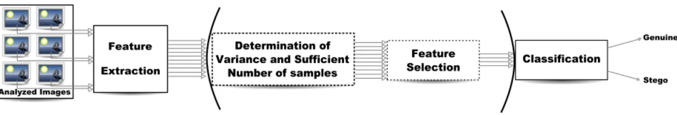
This paper is focused onto classical feature-based steganal-ysis. Such steganalysis typically uses a certain amount of images for training a classifier: features are extracted from the images and fed to a binary classifier (usually Support Vector Machines) for training. The output of this classifier is “stego” (modified using a steganographic algorithm) or “cover” (genuine). This classical process is illustrated on Fig. 1 for the part without parenthesis.
The emphasis in this paper is more specifically on the issues related to the increasing number of features, linked to the universal steganalyzers. Indeed, the very first examples of LSB-based steganalysis made use of less than ten features, with an adapted and specific methodology for each stego algorithm. The idea of “universal steganalyzers” then became
popular. In1999, Westfeld proposes a χ2
-based method, on the LSB of DCT coefficients [30]. Five years after, Fridrich in [6]
uses a set of23 features obtained by normalizations of a much
larger set, whilst Farid et al. already proposed in2002 a set of
72 features [13]. Some feature sets [1] also have variable size
depending on the DCT block sizes. Since then, an increasing number of research works are using supervised learning based
Fig. 1. Overview of the typical global processing for an analyzed image: features are first extracted from the image and then processed through a classifier to decide whether the image is cover or stego. In the proposed processing is added an extra step aimed at reducing the features number and having an additional interpretability of the steganalysis results, by doing a feature selection.
classifiers in very high dimensional spaces. The recent work of Y. Q. Shi et al. [25] is an example of an efficient result but
using324 features based on JPEG blocks differences modeled
by Markov processes. This short survey of some feature sets for steganalysis is by no means exhaustive.
All these results do achieve better and better performance in terms of detection rate and enable to detect most stego algorithm for most embedding rates. Meanwhile, there are some side-effects to this growing number of features. It has been shown for example in [5] that the feature space dimensionality in which the considered classifier is trained, can have a significant impact on its performances: a too small amount of images regarding dimensionality (the number of features) might lead to an improper training of the classifier and thus to results with a possibly high statistical variance.
Comparison of steganalysis methods has been recently pro-posed by Ker [10], by focusing on the pdf of one output of the classifier. In this paper is addressed the idea of a practical way of comparing steganographic schemes, which requires a study on multiple parameters that can influence the performance:
1) the number of images used during the training of the classifier: How to determine a sufficient number of im-ages for an efficient and reliable classification (meaning that final results have acceptable variance)?
2) the number of features used: What are the sufficient and most relevant features for the actual classification problem?
3) the steganography method: Is there an important influ-ence of the stego algorithm on the general methodology? 4) the embedding rate used: Does the embedding rate used for the steganography modifies the variance of the results and the retained best features (by feature selection)? The next section details some of the problems related to the number of features used (dimensionality issues) and commonly encountered in steganalysis: the empty space and the distance concentration phenomena, the important variance of the results obtained by the classifier whenever the number of images used for training is not sufficient regarding the number of features, and finally, the lack of interpretability of the results because of the high number of features. In order to address these issues, the methodology sketched on Fig. 1 is used and more thoroughly detailed: a sufficient number of images regarding the number of features is first established so that the classifier’s training is “reliable” in terms of variance of its results; then, using feature selection the interpretability of the results is improved.
The methodology is finally tested in section IV with six dif-ferents stego algorithms, each using four different embedding rates. Results are finally interpreted thanks to the most relevant selected features for each stego algorithm. A quantitative study of selected features combinations is then provided.
II. DIMENSIONALITY ISSUES ANDMETHODOLOGY
The common term “curse of dimensionality” [2] refers to a wide range of problems related to a high number of features. Some of these dimensionality problems are considered in the following, in relation with the number of images and features.
A. Issues related to the number of images
1) The need for data samples: In order to illustrate this
problem in a low-dimensional case, one can consider four samples in a two dimensional space (corresponding to four images out of which two features have been extracted); the underlying structure leading to the distribution of these four samples seems impossible to infer, and so is the creation of a model for it. Any model claiming it can properly explain the distribution of these samples will behave erratically (because it will extrapolate) when a new sample is introduced. On the contrary, with hundreds to thousands of samples it becomes possible to see clusters and relationships between dimensions. More generally, in order for any tool to be able to analyze and find a structure within the data, the number of needed samples is growing exponentially with the dimensionality.
Indeed, consider a d-dimensional unit side hypercube, the
number of samples needed to fill the Cartesian grid of step
ǫ inside of it is growing as O((1/ǫ)d). Thus using a common
grid of step1/10 in dimension 10, it requires 1010
samples to fill the grid.
In practice, most data sets in steganalysis use at least 10
to 20 dimensions, implying a “needed” number of samples
impossible to achieve: storing and processing such number of images is currently impossible. As a consequence, the feature space is not filled with enough data samples to estimate the density with reliable accuracy; which can give wrong or high variance models when building classifiers, having to extrapolate for the missing samples: results obtained can have rather high confidence interval and hence be statistically
irrelevant. A claim of performance improvement of 2% using
a specific classifier/steganalyzer/steganographic scheme with
2) The increasing variance of the results: The construction
of a proper and reliable model for steganalysis is also related to the variance of the results it obtains. Only experimental results are provided to support this claim: with a low number of images regarding the number of features (a few hundreds of
images for200 features), the variance of the classifier’s results
can be very important.
When the number of images increases, this variance decreases toward proper values for classical steganalysis and performances comparisons. These claims are verified in the next section with the experiments.
3) Proposed solution to the lack of images: Overall, these
two problems lead to the same conclusion: the number of images has to be important, regarding dimensionality. Theory states that this number is exponential with the number of fea-tures, which is impossible to reach for classical steganalysis. Hence, the first step of the proposed methodology is to find a ”sufficient” number of images for the number of features used, according to a criterion on the variance of the results.
A Bootstrap [9] is proposed for that task: the number of images used for the training of the classifier is increased and for each different number of images, the variance of the results of the classifier is assessed. Once the variance of the classifier is below a certain threshold, a sufficient number of images has been found (regarding the classifier and the feature set used).
B. Issues related to the number of features
1) The empty space phenomenon: This phenomenon was
first introduced by Scott and Thompson [24] can be explained with the following example: draw samples from a normal
distribution (zero mean and unit variance) in dimensiond and
consider the probability to have a sample at distancer from the
mean of the distribution (zero). It is given by the probability density function:
f (r, d) = rd−1 2d/2−1.
e−r2/2
Γ(d/2) (2)
having its maximum atr =√d − 1. Thus, when dimension
increases, samples are getting farther from the mean of the distribution. A direct consequence of this is that for the
previ-ously mentionned hypercube in dimensiond, the “center” of it
will tend to be empty, since samples are getting concentrated in the borders and corners of the cube.
Therefore, whatever model is used in such a feature space will be trained on scattered samples which are not filling the feature space at all. The model will then not be proper for any sample falling in an area of the space where the classifier had no information about during the training. It will have to extrapolate its behavior for these empty areas and will have unstable performances.
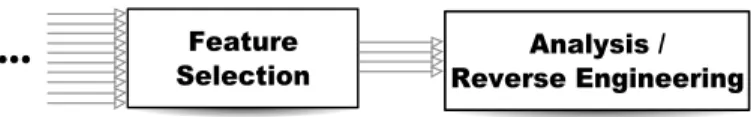
2) Lack of interpretability for possible ”reverse-engineering”: The interpretability (and its applications) is an
important motivation for feature selection and dimensionality reduction: high performances can indeed be reached using the
whole 193 features set used in this paper for classification.
Meanwhile, if looking for the weaknesses and reasons why these features react vividly to a specific algorithm, it seems rather impossible on this important set.
Reducing the required number of features to a small amount through feature selection enables to understand better why a steganographic model is weak on these particular details, high-lighted by the selected features. Such analysis is performed in section IV-C for all six steganographic process.
Fig. 2. Scheme of the possible reverse-engineering on an unknown stego algorithm, by using feature selection for identification of the specific weak-nesses.
Through the analysis of these selected features, one can consider a ”reverse-engineering” of the stego algorithm as illustrated on Fig. 2. By the identification of the most relevant features, the main characteristics of the embedding method can be inferred and the steganographic algorithm be identified if known, or simply understood.
3) Proposed solution to the high number of features: These
two issues motivate the feature selection process: if one can reduce the number of features (and hence the dimensionality), the empty space phenomena will have a reduced impact on the classifier used. Also, the set of features obtained by the feature selection process will give insights on the stego scheme and its possible weaknesses.
For this matter, a classical feature selection technique has been used as the second step of the proposed methodology.
The following methodology is different from the one pre-sented previously in [16], [17]. Indeed, in this article, the goal is set toward statistically reliable results. Also, feature selection has the advantage of reducing the dimensionality of the data (the jumber of features), making the classifier’s training much easier. The interpretation of the selected features is also an important advantage (compared to having only the classifier’s performance) in that it gives insights on the weaknesses of the stego algorithm.
III. METHODOLOGY FOR BENCHMARKING OF
STEGANOGRAPHIC SCHEMES
Addressed problems
The number of data points to be used for building a model and classification is clearly an issue and in the practical case, how many points are needed in order to obtain accurate results – meaning results with small standard deviation.
Reduction of complexity is another main addressed concern in this framework. Then for the selected number of points to be used for classification, and also the initial dimensionality given by the features set, two main steps remain:
• Choosing the feature selection technique. Since analysis
features, the technique used to reduce the dimensionality has to be selected.
• Building a classifier; this implies choosing it, selecting
its parameters, training and validating the chosen model. The following paragraphs presents the solutions for these two major issues, leading to a methodology combining them, presented on Fig. 3.
A. Presentation of the classifier used: OP-ELM
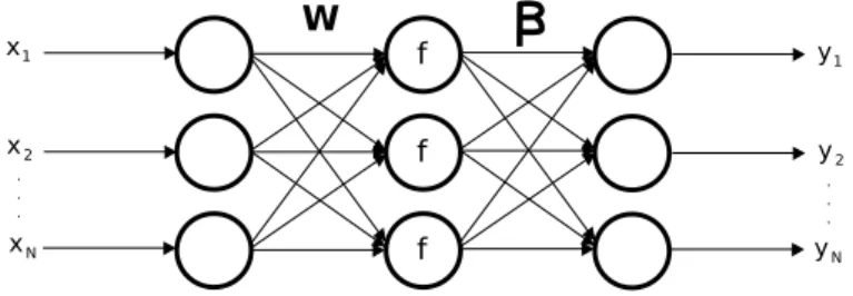
The Optimally-Pruned Extreme Learning Machine (OP-ELM [15], [26]) is a classifier based on the original Ex-treme Learning Machine (ELM) of Huang [8]. This classifier makes use of single hidden layer feedforward neural networks (SLFN) for which the weights and biases are randomly ini-tialized. The goal of the ELM is to reduce the length of the learning process for the neural network, usually very long (for example if using classical back-propagation algorithms). The two main theorems on which ELM is based will not be discussed here but can be found in [8]. Fig. 4 illustrates the typical structure of a SLFN (simplified to a few neurons in here).
Fig. 4. Structure of a classical Single Layer Feedforward Neural Network (SLFN). The input values (the data) X= (x1, . . . , xN) are weighted by the
W coefficients. A possible bias B (not on the figure) can be added to the
weighted inputs wixi. An activation functionf taking this weighted inputs
(plus bias) as input is finally weighted by output coefficientsβ to obtain the
output Y= (y1, . . . , yN).
Supposing the neural network is approximating the output
Y= (y1, . . . , yN) perfectly, we would have: M
X
i=1
βif (wixj+ bi) = yj, j ∈ J1, NK, (3)
withN the number of inputs X = (x1, . . . , xN) (number
of images in our case) and M the number of neurons in the
hidden layer.
As said, the novelty introduced by the ELM is to initialize the weights W and biases B randomly. OP-ELM, in compar-ison to ELM, brings a greater robustness to data with possibly dependent/correlated features. Also, the use of other functions
f (activation functions of the neural network) makes it possible
to use OP-ELM for case where linear components have an important contribution in the classifier’s model, for example.
The validation step of this classifier is performed using classical Leave-One-Out cross-validation, much more precise
than ak-fold cross-validation and hence not requiring any test
step [9]. It has been shown on many experiments [15], [26], that the OP-ELM classifier has results very close to the ones of a Support Vector Machine (SVM) while having computational
times much smaller (usually from10 to 100 times).
B. Determination of a sufficient number of images
A proper number of images, regarding the number of features, has to be determined. Since theoretical values for that number are not reachable, a sufficient number regarding a low enough value of the variance of the results is taken instead (standard deviation will be used instead of variance, in the following).
The OP-ELM classifier is hence used along with a Bootstrap
algorithm [9] over 100 repetitions; a subset of the complete
dataset (10000 images, 193 features) is randomly drawn (with
possible repetitions). The classifier is trained with that specific
subset. This process is repeated100 times (100 random
draw-ings of the subset) to obtain a statistically reliable estimation of the standard deviation of the results. The size of the subset drawn from the complete dataset is then increased, and the
100 iterations are repeated for this new subset size.
The criterion to stop this process is a threshold on the value of the standard deviation of the results. Once the standard
deviation of the results gets lower than1%, it is decided that
the subset size S giving such low standard deviation of the
classifier’s results, is sufficient. S is then used for the rest of
the experiments as a sufficient number of images regarding the number of features in the feature set.
C. Dimensionality reduction: feature selection by Forward with OP-ELM
Given the sufficient number of images for reliable training
of the classifier, S, feature selection can be performed. The
second step of the methodology, a Forward algorithm with OP-ELM (Fig. 3) is used.
1) The Forward algorithm: The forward selection
algo-rithm is a greedy algoalgo-rithm [22]; it selects one by one the dimensions, trying to find the one that combines best with the
already selected ones. The algorithm is (with xi denoting the
i-th dimension of the data set)
Algorithm 1 Forward
R= {xi, i ∈ J1, dK} S= ∅
while R6= ∅ do forxj∈ R do
Evaluate performance with S∪ xj
end for
Set S= S ∪ {xk}, R = R − xk withxk the dimension
giving the best result in the loop
end while
This algorithm requires d(d − 1)
2 instances to terminate (to
be compared to the2d− 1 instances for an exhaustivesearch),
which might reach the computational limits, depending on the number of dimensions and time to evaluate the performance with one set. With the OP-ELM as a classifier, computational times are not much of an issue.
Even if its capacity to isolate efficient features is clear, the forward technique has some drawbacks. First, if two features present good results when put together but poor results if only
Bootstrap
Fig. 3. Schematic view of the proposed methodology: (1) An appropriate number of data samples to work with is determined using a Bootstrap method for statistical stability; (2) The forward selection is performed using an OP-ELM classifier to find a good features set. Follows a possible interpretation of the features or the typical classification for steganalysis.
one of them is selected, forward might not take these into account in the selection process.
Second, it does not allow to “go back” in the process, mean-ing that if performances are decreasmean-ing along the selection process, and that the addition of another feature makes per-formances increase again, combinations of previously selected features with this last one are not possible anymore.
The Forward selection is probably not the best possible feature selection technique, and recent contribution to these techniques such as Sequential Floating Forward Selection (SFFS) [27] and improvements of it [4] have shown that the number of computations required for feature selection can be reduced drastically. Nevertheless, the feature selection using Forward has been showing very good results and seems to perform well on the feature set used in this paper. It is not used here in the goal of obtaining the best possible combination of features, but more to reduce the dimensionality and obtain some meaning out of the selected features. Improvements of this methodology could make use of such more efficient techniques of feature selection.
D. General Methodology
To summarize, the general methodology on Fig. 3 uses
first a Bootstrap with100 iterations on varying subsets sizes,
to obtain a sufficient subset size and statistically reliable classifiers’ results, regarding the number of features used. With this number of images, feature selection is performed using a Forward selection algorithm; this enables to highlight possible weaknesses of the stego algorithm.
This methodology has been applied to six popular stego algorithms for testing. Experiments and results, as well as a discussion on the analysis of the selected features are given in the next section.
IV. EXPERIMENTS AND RESULTS
A. Experiments setup
1) Steganographic algorithms used: Six different steganographic algorithms have been used: F5 [29], Model-Based (MBSteg) [23], MMx [11] (in these experiments, MM3 has been used), JP Hide and Seek [12], OutGuess [20], StegHide [7]; all of them with four different embedding rates:
5, 10, 15 and 20%.
2) Generation of image database: The image base was
constituted of10000 images from the BOWS2 Challenge [18]
database (hosted by Andreas Westfeld [28]). These images are
512 × 512 PGM greyscale (also available in color).
While the steganographic processes and the proposed methodology for dimensionality reduction and steganalysis
are only performed on these 512 × 512 images, any size of
image would work just as well.
3) Extraction of the features: In the end, the whole set
of images is separated in two equal parts: one is kept as untouched cover while the other one is stego with the six steganographic algorithms at four different embedding rates:
5%, 10%, 15% and 20%. Fridrich’s 193 DCT features [19]
have been used for the steganalysis.
B. Results
Results are presented following the methodology steps. A discussion over the selected features and the possible interpretability of it are developed afterward. In the following, the term ”detection rate” stands for the performance of the
classifier on a scale from 0 to 100% of classification rate.
It is a measure of the performance instead of a measure of error.
1) Determination of sufficient number of samples:
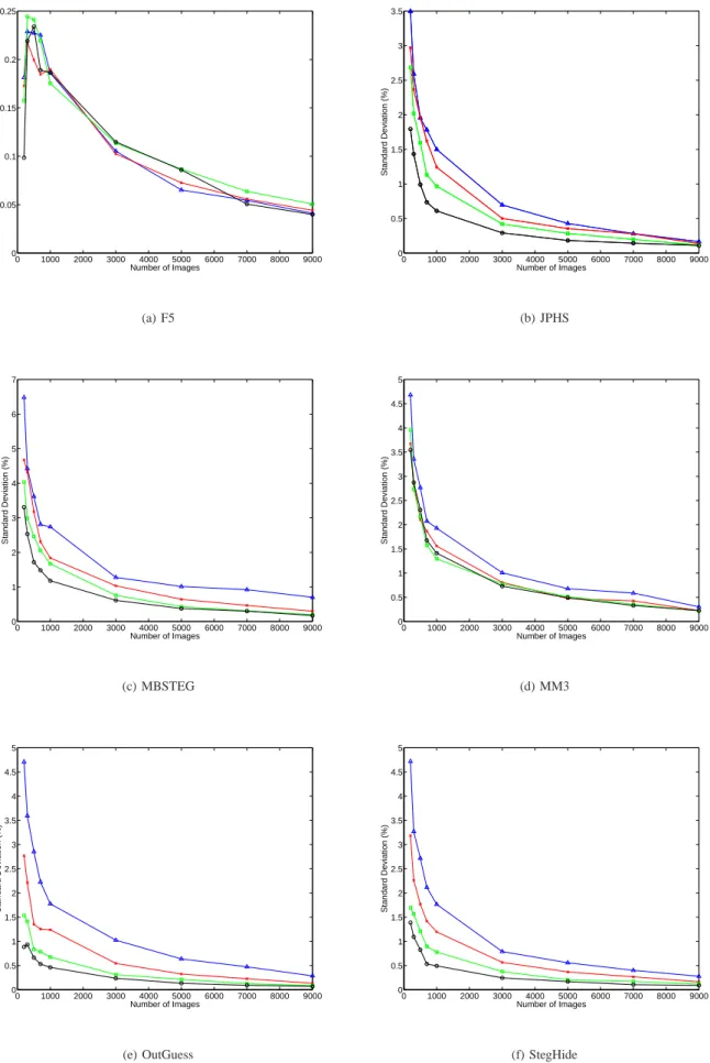
Pre-sented first is the result of the evaluation of a sufficient number of images, as explained in the previous methodology, on Fig. 5.
The Bootstrap (100 rounds) is used on randomly taken subsets
of 200 up to 9000 images out of the whole 10000 from the
BOWS2 challenge.
It can be seen on Fig. 5 that the standard deviation behaves as expected when increasing the number of images, for the cases of JPHS, MBSteg, MMx, OutGuess and StegHide: its
value decreases and tends to below1% of the best performance
when the number of images is5000 (even if for MBSteg with
embedding rate of 5% it is a bit above 1%). This sufficient
number of samples is kept as the reference and sufficient num-ber. Another important point is that with very low number of
images (100 in these cases), the standard deviation is between
1 and about 6.5% of the average classifier’s performance;
meaning that results computed with as small number of images
have at most a ±6.5% confidence interval. While the plots
decrease very quickly when increasing the number of images,
0 1000 2000 3000 4000 5000 6000 7000 8000 9000 0 0.05 0.1 0.15 0.2 0.25 Number of Images Standard Deviation (%) (a) F5 0 1000 2000 3000 4000 5000 6000 7000 8000 9000 0 0.5 1 1.5 2 2.5 3 3.5 Number of Images Standard Deviation (%) (b) JPHS 0 1000 2000 3000 4000 5000 6000 7000 8000 9000 0 1 2 3 4 5 6 7 Number of Images Standard Deviation (%) (c) MBSTEG 0 1000 2000 3000 4000 5000 6000 7000 8000 9000 0 0.5 1 1.5 2 2.5 3 3.5 4 4.5 5 Number of Images Standard Deviation (%) (d) MM3 0 1000 2000 3000 4000 5000 6000 7000 8000 9000 0 0.5 1 1.5 2 2.5 3 3.5 4 4.5 5 Number of Images Standard Deviation (%) (e) OutGuess 0 1000 2000 3000 4000 5000 6000 7000 8000 9000 0 0.5 1 1.5 2 2.5 3 3.5 4 4.5 5 Number of Images Standard Deviation (%) (f) StegHide
Fig. 5. Standard deviation in percentage of the average classification result versus the number of images, for all six steganographic algorithms, for the four embedding rates: black circles ( ) for20%, green squares (2) for15%, red crosses (×) for10% and blue triangles (a) for5%. These estimations have
images; these results have to take into account the embedding rate, which tends to make the standard deviation higher as it decreases.
Indeed, while differences between15 and 20% embedding
rates are not very important on the four previously mentioned
stego algorithms, there is a gap between the 5 − 10% plots
and the 20% ones. This is expected when looking at the
performances of the steganalysis process: low embedding rates tend to be harder to detect, leading to a range of possible performances wider than with high embedding rates. Fig. 6 illustrates this idea on the cases of JPHS, MMx, MBSteg StegHide and OutGuess (the F5 results are behaving differ-ently on these plots; this is discussed below).
Finally, the F5 algorithm have ”erratic” behaviour, on Fig. 5. This can be explained by the very high performance of the
classifier (close to100%) and hence, the very small possible
standard deviation: it ranges between0.25% and 0.05%. It is
then no surprise that the plots have such an erratic behaviour. The final “sufficient” number of samples retained for the second step of the methodology – the feature selection – is 5000, for two reasons: first, the computational times are
acceptable for the following computations (feature selection step with training of classifier for each step); second, the standard deviation is small enough to consider that the final
classification results are given with at most 1% of standard
deviation (in the case of MBSteg at5% of embedding rate).
2) Forward feature selection: Features have first been
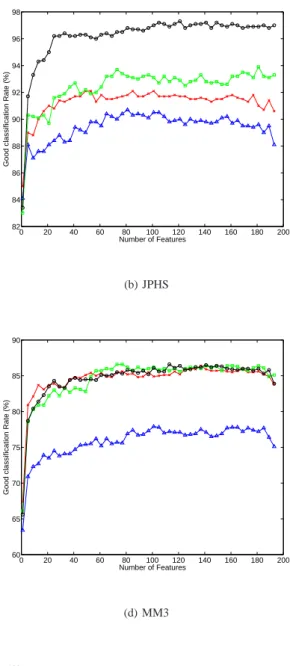
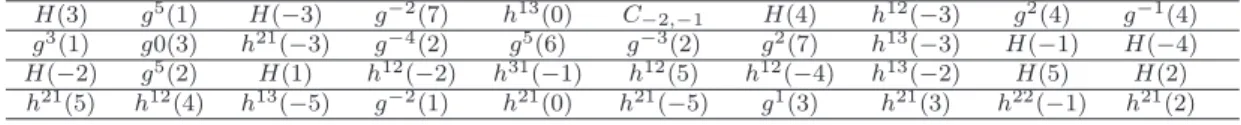
ranked, using the Forward feature selection algorithm, and detection rates are plotted with increasing number of features (using the ranking provided by the Forward selection) on Fig. 6.
F5 case is different again: whatever the embedding rate
used, steganalysis is surprisingly easy: using as low as 1
feature for all embedding rates, detection rate is 100% even
with only5% embedding rate.
The five other analyzed stego algorithms give rather differ-ent results:
• JPHS reaches a plateau in performance (within the
stan-dard deviation of 1%) for all embedding rates with
41 features and remains around that performance, even
though performances are quite ”unstable”
• OutGuess has this same plateau at25 features and
perfor-mances are not increasing anymore above that number of features (stll within the standard deviation of the results)
• StegHide can be considered to have reached the
maxi-mum result (within the standard deviation interval) at60
features, even if for 5% embedding rate, performances
keep on increasing while adding features. . .
• In the MM3 case, performances for embedding rates
10, 15 and 20% are very similar as are selected features.
Performances stable at40 features.
• Performances for MBSteg are stable using 70 features
for embedding rates15 and 20%. Only 30 are enough for
embedding rate5%. The case of embedding rate 10% has
the classifier’s performances increasing with the addition of features.
Interestingly, the features retained by the forward selection
for each embedding rate differ slightly, within one stegano-graphic algorithm. Details about the features ranked as first by the Forward algorithm are discussed afterward.
C. Discussion
First, the global performances when using the reduced and sufficient feature sets mentioned in the results section above, are assessed. Note that feature selection for performing reverse-engineering of a steganographic algorithm is theo-retically efficient only if the features are carrying different information (if two features represent the same information, the feature selection will select only one of them).
1) Reduced features sets: Based on the ranking of the
features obtained by the Forward algorithm, it has been
decided that once performances were within 1% of the best
performance obtained (among all Forward tryouts for all different sets of features), the number of features obtained was retained as a ”sufficient” feature set. Performances using reduced feature sets (proper to each algorithm and embedding rate) are first compared in Table I.
5% # 10% # F5 100.0 1 100.0 1 JPHS 90.7 41 92.1 21 MBSteg 63.3 57 70.9 93 MM3 78.00 81 86.2 49 OutGuess 81.2 65 93.2 49 Steghide 82.3 149 91.2 89 15% # 20% # F5 100.0 1 100.0 1 JPHS 93.7 41 97.3 25 MBSteg 83.5 73 88.5 69 MM3 86.6 57 86.6 73 OutGuess 98.8 33 100.0 29 Steghide 96.4 73 99 73 TABLE I
PERFORMANCES FOROP-ELM LOOFOR THE BEST FEATURES SET ALONG WITH THE SIZE OF THE REDUCED FEATURE SET(#). PERFORMANCES USING THE REDUCED SET ARE WITHIN THE1%RANGE OF STANDARD DEVIATION OF THE BEST RESULTS. THE SIZE OF THE SET HAS BE DETERMINED TO BE THE SMALLEST POSSIBLE ONE GIVING THIS
PERFORMANCE.
It should be noted that since the aim of the feature selection is to reduce as much as possible the feature set while keeping overall same performance, it is expected that within the standard deviation interval, the performance with the lowest possible number of features is behind the “maximum” one.
It remains possible, for the studied algorithms, as Fig. 6 shows, to find a higher number of features for which the performance is closer or equal to the maximum one – even
though this is very disputable, considering the maximal 1%
standard deviation interval when using5000 images. But this
is not the goal of the feature selection step of the methodology.
D. Feature sets analysis for reverse-engineering
Common feature sets have been selected according to the following rule: take the first common ten features (in the order ranked by the Forward algorithm) to each feature set obtained for each embedding rate (within one algorithm). It
0 20 40 60 80 100 120 140 160 180 200 99.4 99.5 99.6 99.7 99.8 99.9 100 Number of Features
Good classification Rate (%)
(a) F5 0 20 40 60 80 100 120 140 160 180 200 82 84 86 88 90 92 94 96 98 Number of Features
Good classification Rate (%)
(b) JPHS 0 20 40 60 80 100 120 140 160 180 200 55 60 65 70 75 80 85 90 Number of Features
Good classification Rate (%)
(c) MBSTEG 0 20 40 60 80 100 120 140 160 180 200 60 65 70 75 80 85 90 Number of Features
Good classification Rate (%)
(d) MM3 0 20 40 60 80 100 120 140 160 180 200 60 65 70 75 80 85 90 95 100 Number of Features
Good classification Rate (%)
(e) OutGuess 0 20 40 60 80 100 120 140 160 180 200 55 60 65 70 75 80 85 90 95 100 Number of Features
Good classification Rate (%)
(f) StegHide
Fig. 6. Performance in detection for all six stego algorithms versus the number of features, for the four embedding rates: black circles ( ) for20%, green
squares (2) for15%, red crosses (×) for10% and blue triangles (a) for5%. Features are ranked using the Forward selection algorithm. These plots are the
is hoped that through this selection, the obtained features will be generic regarding the embedding rate.
The F5 case is discarded, since only one feature makes it
possible to achieve99% of detection rate, that is the Global
Histogram of coefficient3: H(3) in the following notation.
Notations for the feature set used [19] are first given for the
original23 features set, in Table II:
Functional/Feature Functional F Global histogram H/||H|| Individual histogram h21/||h21 ||,h12 /||h12 ||,h13 /||h13 ||, for 5 DCT Modes h22/||h22||,h31/||h31||
Dual histogram for g−5/||g−5||,g−4/||g−4||,. . . ,
11 DCT values g4 /||g4 ||,g5 /||g5 || Variation V L1 and L2 blockiness B1, B2 Co-occurrence N00,N01,N11 TABLE II
THE23FEATURES PREVIOUSLY DETAILED.
This set of23 features is expanded up to a set of 193, by
removing theL1norm used previously and keep all the values
of the matrices and vectors. This results in the following193
features set:
• A global histogram of 11 dimensions H(i), i = J−5, 5K
• 5 low frequency DCT histograms each of 11 dimensions
h21
(i) . . . h31
(i), i = J−5, 5K
• 11 dual histograms each of 9 dimensions
g−5(i) . . . g5
(i), i = J1, 9K
• Variation of dimension 1 V
• 2 blockinesses of dimension 1 B1, B2
• Co-occurrence matrix of dimensions 5 × 5 Ci,j, i =
J−2, 2K, j = J−2, 2K
Follows a discussion on the selected features for each steganographic algorithm.
Tables of selected feature sets are presented below, with an analysis of it for each algorithm. Fridrich’s DCT features are not the only ones having a possible physical interpretation. They have been chosen here because it is believed that most of the features can be interpreted. The proposed short analysis of the weaknesses of stego algorithms is using this interpretation.
h21(1) h21(2) h12(0) h12(2) h22(1)
g−5(1) C
−2,−1 C−1,+1 C−1,+2 C+0,−2
TABLE III
COMMON FEATURE SET FORMM3.
1) MM3: MM3 tends to be very sensitive to coefficients
histograms features, which they do not preserve. Low DCT
coefficients values (−1, +1) are found for MM3. Interestingly,
co-occurrence coefficients react for MM3, as well as for JPHS (in the following) but only these two stego algorithms.
h12(2) h12(3) h13(1) h22(1) h31(1)
h12(2) C
−2,−1 C−1,+1 C−1,+2 C+0,+1
TABLE IV
COMMON FEATURE SET FORJPHS.
2) JPHS: JPHS seems not to preserve the low and medium
frequencies coefficients and also not the frequency coherence (from the co-occurrence matrix). Also, DCT coefficients his-tograms are not preserved.
H(−1) H(1) H(3) h21(0) h21(1)
h21(3) h12(−1) h12(0) h12(1) h12(−5)
TABLE V
COMMON FEATURE SET FORMBSTEG.
3) MBSteg: The features used (Table V) include global
histograms with values 0,−2 and 2, which happens only
because of the calibration in the feature extraction process. MBSteg preserves the coefficients’ histograms but does not take into account a possible calibration. Hence, the unpre-served histograms are due to the calibration process in the feature extraction. Information leaks through the calibration process. h21(−1) h21(0) h21(2) h12(−1) h12(0) h13 (−1) h13 (0) h13 (1) h22 (−1) h22 (1) TABLE VI
COMMON FEATURE SET FOROUTGUESS.
4) OutGuess: Extreme values histograms are mostly used
(values−2, −1) in the feature set for OutGuess (Table VI) and
a clear weak point. The calibration process has indeed been
of importance since the histogram of value0 has been taken
into account. h21(−1) h21(0) h12(1) h12(3) h13(−1) h13 (0) h13 (1) h22 (1) h31 (−1) h31 (0) TABLE VII
COMMON FEATURE SET FORSTEGHIDE.
5) StegHide: For StegHide (Table VII), histograms are
mostly used, with high frequencies coefficients (31, 13, 22)
and for low values (between−1 and +1).
From a general point of view, we can notice that all the analysed algorithms are very sensitive to statistics of low-pass calibrated DCT coefficients, which are represented by features
h21
and h12
. This is not surprising since these coefficients contain a large part of the information of a natural image, their associated densities are likely to be modified by the embedding process. Note that fooling this process by embedding only inside the high-frequency coefficients is possible but reduces considerably the embedding payload.
V. CONCLUSIONS
This paper has presented a methodology for the estimation of a sufficient number of images for a specific feature set using the standard deviation of the detection rate obtained by the classifier as a criterion (a Bootstrap technique is used for that purpose); the general methodology presented can nonetheless be extended and applied to other feature sets. The second step of the methodology aims at reducing the
dimensionality of the data set, by selecting the most relevant features, according to a Forward selection algorithm; along with the positive effects of a lower dimensionality, analysis of the selected features is possible and gives insights on the steganographic algorithm studied.
Three conclusions can be drawn from the methodology and experiments in this paper:
• Results on standard deviation for almost all studied
steganographic algorithms have proved that the feature-based steganalysis is reliable and accurate only if a sufficient number of images is used for the actual training of the classifier used. Indeed, from most of the results obtained concerning standard deviation values (and therefore statistical stability of the results), it is rather irrelevant to possibly increase detection performance by
2% while working with a standard deviation for these
same results of2%.
• Through the second step of the methodology, the required
number of features for steganalysis can be decreased. This with three main advantages: (a) performances remain the same if the reduced feature set is properly constructed; (b) the selected features from the reduced set are relevant and meaningful (the selected set can possibly vary, according to the feature selection technique used) and make reverse-engineering possible; (c) the weaknesses of the stego algorithm also appear from the selection; this can lead for example to improvements of the stego algorithm.
• The analysis on the reduced common feature sets
obtained between embedding rates of the same stego algorithm, shows that the algorithms are sensitive to roughly the same features, as a basis. Meanwhile, when
embedding rates get as low as 5%, or for very efficient
algorithms, some very specific features appear.
Hence, the first step of the methodology is a require-ment for any new stego algorithm, but also new feature sets/steganalyzers, willing to present its performances: a suf-ficient number of images for the stego algorithm and the steganalyzer used to test it has to be assessed in order to have stable results (that is, with a small enough standard deviation of its results to make the comparison with current state of the art techniques meaningful).
Also, from the second step of the methodology, the most relevant features can be obtained and make possible a further analysis of the stego algorithm considered, additionally to the detection rate obtained by the steganalyzer.
ACKNOWLEDGEMENTS
The authors would like to thank Jan Kodovsky and Jessica Fridrich for their implementation of the DCT Feature Extrac-tion software.
REFERENCES
[1] S. S. Agaian and H. Cai. New multilevel dct, feature vectors, and universal blind steganalysis. In IS&T/SPIE 17th Annual Symposium
Electronic Imaging Science and Technology; Security, Steganography, and Watermarking of Multimedia Contents VI, page 12, January 2005.
[2] R. Bellman. Adaptive control processes: a guided tour. Princeton University Press, 1961.
[3] C. Cachin. An information-theoretic model for steganography. In
In-formation Hiding: 2nd International Workshop, volume 1525 of Lecture Notes in Computer Science, pages 306–318, 14-17 April 1998.
[4] EURASIP, editor. Fast Sequential Floating Forward Selection applied
to Emotional Speech Features estimated on DES and SUSAS Data Collections. Eusipco signal processing conference, 2006.
[5] D. Franc¸ois. High-dimensional data analysis: optimal metrics and
fea-ture selection. PhD thesis, Universit´e catholique de Louvain, September
2006.
[6] J. Fridrich. Feature-based steganalysis for jpeg images and its impli-cations for future design of steganographic schemes. In Information
Hiding: 6th International Workshop, volume 3200 of Lecture Notes in Computer Science, pages 67–81, May 23-25 2004.
[7] S. Hetzl and P. Mutzel. A graph-theoretic approach to steganography. In Dittmann J., Katzenbeisser S., and Uhl A., editors, CMS 2005, Lecture Notes in Computer Science 3677, pages 119–128. Springer-Verlag, 2005. [8] G.-B. Huang, Q.-Y. Zhu, and C.-K. Siew. Extreme learning machine: Theory and applications. Neurocomputing, 70(1–3):489–501, December 2006.
[9] B. Efron R. J. and Tibshirani. An Introduction to the Bootstrap. Chapman et al., Londres, 1994.
[10] A. D. Ker. The ultimate steganalysis benchmark? In 9th ACM
Multimedia and Security Workshop, 2007.
[11] Y. Kim, Z. Duric, and D. Richards. Modified matrix encoding technique for minimal distortion steganography. In Information Hiding 2007, volume 4437/2007, pages 314–327, 2007.
[12] A. Latham. Jphide&seek, August 1999. http://linux01.gwdg.de/ alatham/stego.html.
[13] S. Lyu and H. Farid. Detecting hidden messages using higher-order statistics and support vector machines. In 5th International Workshop
on Information Hiding, Noordwijkerhout, The Netherlands, 2002.
[14] D. McCullagh. Secret Messages Come in .Wavs. Online Newspaper: Wired News, February 2001. http://www.wired.com-/news/politics/ 0,1283,41861,00.html.
[15] Y. Miche, P. Bas, C. Jutten, O. Simula, and A. Lendasse. A methodology for building regression models using extreme learning machine: OP-ELM. In ESANN 2008, European Symposium on Artificial Neural
Networks, Bruges, Belgium, April 23-25 2008. to be published.
[16] Y. Miche, P. Bas, A. Lendasse, C. Jutten, and O. Simula. Extracting rele-vant features of steganographic schemes by feature selection techniques. In Wacha’07: Third Wavilla Challenge, June 14 2007.
[17] Y. Miche, B. Roue, P. Bas, and A. Lendasse. A feature selection methodology for steganalysis. In MRCS06, International Workshop
on Multimedia Content Representation, Classification and Security, Istanbul (Turkey), Lecture Notes in Computer Science. Springer-Verlag,
September 11-13 2006.
[18] Watermarking Virtual Laboratory (Wavila) of the European Network of Excellence ECRYPT. The 2nd bows contest (break our watermarking system), 2007.
[19] T. Pevny and J. Fridrich. Merging markov and dct features for multi-class jpeg steganalysis. In IS&T/SPIE 19th Annual Symposium
Electronic Imaging Science and Technology, volume 6505 of Lecture Notes in Computer Science, January 29th - February 1st 2007.
[20] N. Provos. Defending against statistical steganalysis. In 10th USENIX
Security Symposium, pages 323–335, 13-17 April 2001.
[21] N. Provos and P. Honeyman. Detecting steganographic content on the internet. In Network and Distributed System Security Symposium. The Internet Society, 2002.
[22] F. Rossi, A. Lendasse, D. Franc¸ois, V. Wertz, and M. Verleysen. Mutual information for the selection of relevant variables in spectrometric nonlinear modelling. Chemometrics and Intelligent Laboratory Systems, 80:215–226, 2006.
[23] P. Sallee. Model-based steganography. In Digital Watermarking, volume 2939/2004 of Lecture Notes in Computer Science, pages 154–167. Springer Berlin / Heidelberg, 2004.
[24] D. Scott and J. Thompson. Probability density estimation in higher dimensions. In S.R. Douglas, editor, Computer Science and Statistics:
Proceedings of the fifteenth symposium on the interface, pages 173–179,
[25] Y. Q. Shi, C. Chen, and W. Chen. A markov process based approach to effective attacking jpeg steganography. In ICME’06 : Internation
Conference on Multimedia and Expo, Lecture Notes in Computer
Science, 9-12 July 2006.
[26] A. Sorjamaa, Y. Miche, and A. Lendasse. Long-term prediction of time series using nne-based projection and op-elm. In IJCNN2008:
International Joint Conference on Neural Networks, June 2008. to be
published.
[27] D. Ververidis and C. Kotropoulos. Fast and accurate sequential floating forward feature selection with the bayes classifier applied to speech emotion recognition. Signal Processing, 88(12):2956–2970, December 2008.
[28] A. Westfeld. Reproducible signal processing (bows2 challenge image database, public).
[29] A. Westfeld. F5-a steganographic algorithm. In Information Hiding:
4th International Workshop, volume 2137, pages 289–302, 25-27 Avril
2001.
[30] A. Westfeld and A. Pfitzmann. Attacks on steganographic systems. In
IH ’99: Proceedings of the Third International Workshop on Information Hiding, pages 61–76, London, UK, 2000. Springer-Verlag.
APPENDIX:FEATURES RANKED BY THEFORWARD ALGORITHM
As appendix are given the first40 features obtained by the
Forward ranking for each stego algorithm with5% embedding
rate. Only one embedding rate result is given for space
reasons. 5% embedding rate results have been chosen since
they tend to be different (in terms of ranked features by the Forward algorithm) from the other embedding rates and also
because 5% embedding rate is a difficult challenge in terms
of steganalysis; these features are meaningful for this kind of difficult steganalysis with these six algorithms.
H(3) g5 (1) H(−3) g−2(7) h13(0) C −2,−1 H(4) h 12 (−3) g2 (4) g−1(4) g3(1) g0(3) h21(−3) g−4(2) g5(6) g−3(2) g2(7) h13(−3) H(−1) H(−4) H(−2) g5 (2) H(1) h12 (−2) h31 (−1) h12 (5) h12 (−4) h13 (−2) H(5) H(2) h21(5) h12(4) h13(−5) g−2(1) h21(0) h21(−5) g1(3) h21(3) h22(−1) h21(2) TABLE VIII
THE40FIRST FEATURES RANKED BY THEFORWARD ALGORITHM FOR THEF5ALGORITHM AT5%EMBEDDING RATE.
g0(4) h22(0) C 1,0 B1 H(1) h21(0) g1(4) g0(8) g−2(9) g−2(5) g4 (5) g0 (5) g1 (9) g−1(2) B2 g2(8) C0,0 h31(5) g0(9) h22(1) g−2(2) g−1(7) g−3(8) g0(1) h31(−3) h21(−1) h22(−1) g−4(6) C −1,−2 g 5(7) h12(−5) g−5(8) h21(2) g0(7) h12(−2) h22(−4) h31(0) C0,2 H(2) g5(5) TABLE IX
THE40FIRST FEATURES RANKED BY THEFORWARD ALGORITHM FOR THEJPHSALGORITHM AT5%EMBEDDING RATE.
g−2(1) H(2) g−4(7) h13(1) h22(1) C2,−2 C −1,−1 h 31 (1) g4 (7) g−2(4) h21(0) h31(−4) h21(−4) C 0,2 C12 h31(−1) H(0) h21(3) g−5(6) h22(−3) h13(−1) C 2,0 C1,2 g5(6) C−2,−1 g−3(6) g 5(4) g−2(7) g−1(7) g−4(8) h22 (−1) g2 (1) g0 (8) h22 (−5) H(−2) h12 (−4) g5 (5) h12 (−2) g2 (4) h21 (−3) TABLE X
THE40FIRST FEATURES RANKED BY THEFORWARD ALGORITHM FOR THEMBSTEG ALGORITHM AT5%EMBEDDING RATE.
C−1,−1 h 13(−1) C 0,−2 C1,1 g0(9) C2,0 h21(−1) h13(1) g−3(2) C10 H(−2) g4(4) g2(2) C −2,0 C0,−1 C−1,−2 g−2(3) h 22(−3) g2(3) h13(3) h31 (−1) g−1(9) g−2(8) g0(7) h21(−5) h21(3) C −1,1 g−1(3) g 5 (3) h31 (1) g0(3) B1 C −2,1 B2 g−4(6) C0,2 H(−1) g 2(5) h13(0) g2(7) TABLE XI
THE40FIRST FEATURES RANKED BY THEFORWARD ALGORITHM FOR THEMM3ALGORITHM AT5%EMBEDDING RATE.
h13 (0) C0,−1 C−2,0 H(−2) B1 C0,−2 g 0 (7) h31 (−3) C−2,−1 g 0 (2) B2 H(−1) g−2(2) h13(−1) h22(−1) h22(0) h12(−3) g−2(5) g1(8) h21(−2) g−2(9) g1(1) H(5) H(4) g2(1) g0(1) g−3(5) g0(9) g−3(8) g−3(3) g−5(4) g−5(5) C −2,−2 g−1(6) g−2(6) g 4 (3) C−1,−1 C−1,0 g−2(7) C−1,1 TABLE XII
THE40FIRST FEATURES RANKED BY THEFORWARD ALGORITHM FOR THEOUTGUESS ALGORITHM AT5%EMBEDDING RATE.
C0,−1 g0(2) C0,2 C2,−2 B1 B2 C1,1 C0,−2 C−2,2 h 13(−1) g−5(3) h21(−3) C 0,1 h13(0) C1,−1 h31(−1) g−3(3) g3(6) h31(−2) g1(3) h22 (1) C−2,−2 g−4(4) h 13 (1) C−2,0 g 1 (4) C2,1 H(−1) C2,2 h22(5) g2(5) C −1,−1 g 1(9) C 2,0 g2(7) g−1(1) h31(5) H(−2) h21(1) g−2(9) TABLE XIII